Reinforcement Learning from Demonstration

Worcester Polytechnic Institute

Digital WPI

Doctoral Dissertations (All Dissertations, All Years)

Electronic Theses and Dissertations

2016-04-25

Reinforcement Learning from Demonstration

Halit Bener Suay

Worcester Polytechnic Institute

Follow this and additional works at:

https://digitalcommons.wpi.edu/etd-dissertations

This dissertation is brought to you for free and open access byDigital WPI. It has been accepted for inclusion in Doctoral Dissertations (All Dissertations, All Years) by an authorized administrator of Digital WPI. For more information, please [email protected].

Repository Citation

Suay, H. B. (2016).Reinforcement Learning from Demonstration. Retrieved fromhttps://digitalcommons.wpi.edu/etd-dissertations/ 173

4/22/16

4/20/2016

• • • •

12/17/2010 7:25 PM FROM: Inland Inland Diamond Products TO: 16103305059 PAGE: 001 OF 003

To: Fax number: From: Fax number: Business phone: Home phone: Date & Time: Pages: Re:

•

• Inland Diamond Products

• • • • • • • • * 16103305059 Sandy Banks 248/585-0499 248/585-2330 X12 12/17/20107:25:18 PM 3

Fax from Sandy Banks

c

Copyright by Halit Bener Suay 2016 All rights reserved

Abstract

Off-the-shelf Reinforcement Learning (RL) algorithms suffer from slow learning per-formance, partly because they are expected to learn a task from scratch merely through an agent’s own experience. In this thesis, we show that learning from scratch is a lim-iting factor for the learning performance, and that when prior knowledge is available RL agents can learn a task faster. We evaluate relevant previous work and our own algorithms in various experiments.

Our first contribution is the first implementation and evaluation of an existing inter-active RL algorithm in a real-world domain with a humanoid robot. Interinter-active RL was evaluated in a simulated domain which motivated us for evaluating its practicality on a robot. Our evaluation shows that guidance reduces learning time, and that its positive effects increase with state space size.

A natural follow up question after our first evaluation was, how do some other previous works compare to interactive RL. Our second contribution is an analysis of a user study, where na¨ıve human teachers demonstrated a real-world object catching with a humanoid robot. We present the first comparison of several previous works in a common real-world domain with a user study.

One conclusion of the user study was the high potential of RL despite poor usabil-ity due to slow learning rate. As an effort to improve the learning efficiency of RL learners, our third contribution is a novel human-agent knowledge transfer algorithm. Using demonstrations from three teachers with varying expertise in a simulated do-main, we show that regardless of the skill level, human demonstrations can improve the asymptotic performance of an RL agent.

As an alternative approach for encoding human knowledge in RL, we investigated the use of reward shaping. Our final contributions are Static Inverse Reinforcement Learning Shaping and Dynamic Inverse Reinforcement Learning Shaping algorithms that use human demonstrations for recovering a shaping reward function. Our experi-ments in simulated domains show that our approach outperforms the state-of-the-art in cumulative reward, learning rate and asymptotic performance.

Overall we show that human demonstrators with varying skills can help RL agents to learn tasks more efficiently.

Acknowledgments

Research presented in different chapters of this thesis was supported by Worcester Polytechnic Institute, NSF Award 1149876, ONR Award N00014-14-1-0795. This research has taken place in part at the Intelligent Robot Learning (IRL) Lab, Wash-ington State University and research presented in Chapter 6 was supported in part by grants AFRL FA8750-14-1-0069, AFRL FA8750-14-1-0070, NSF IIS-1149917, NSF IIS-1319412, USDA 2014-67021-22174, and a Google Research Award.

Contents

1 Introduction 1

1.1 Contributions and Overview . . . 3

2 Background 5 2.1 Learning from Demonstration . . . 5

2.2 Reinforcement Learning . . . 7

2.3 Inverse Reinforcement Learning . . . 10

2.4 Transfer Learning . . . 13

2.5 Reward Shaping . . . 15

2.6 Reinforcement Learning from Demonstration . . . 16

3 Effect of Human Guidance and State Space Size on Interactive Reinforcement Learning 18 3.1 Overview . . . 19

3.2 Description of Interactive RL Algorithm . . . 20

3.3 Experimental Setup . . . 23

3.3.1 Domain . . . 23

3.3.2 Experimental Conditions . . . 25

3.4 Results . . . 28

3.5 Discussion . . . 29

4 A Comparison of Three Learning from Demonstration Algorithms 33 4.1 Overview . . . 33

4.2 Description of Selected LfD Algorithms . . . 35

4.3 Evaluation . . . 37 4.3.1 User Study . . . 38 4.3.2 Experimental Setup . . . 39 4.4 Qualitative Results . . . 41 4.5 Quantitative Results . . . 46 4.6 Discussion . . . 53

5 Human-Agent Transfer: HAT 57 5.1 Overview . . . 58

5.3 Evaluation . . . 61

5.3.1 Keepaway . . . 62

5.3.2 Experimental Setup . . . 63

5.4 Results . . . 65

5.5 Discussion . . . 73

6 Learning from Demonstration for Shaping through Inverse Reinforcement Learning 75 6.1 Overview . . . 75 6.2 Methodology . . . 78 6.3 Experimental Validation . . . 82 6.3.1 Maze . . . 83 6.3.2 Mario AI . . . 88 6.4 Discussion . . . 93

List of Tables

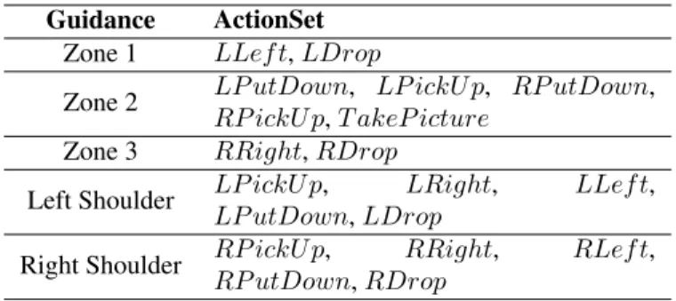
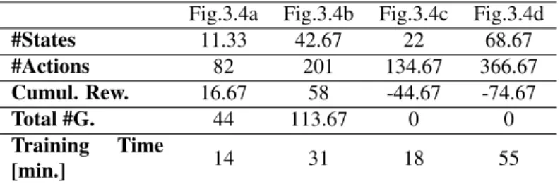
3.1 Guidance messages restrict action selection to the set of available ac-tions as shown. The first letter LandRdenotes either Left or Right hand depending on the hand with which the action is executed. . . 25 3.2 Experiment statistics. All results are shown as the average of three

tri-als for each experiment. Number of states discovered (#States), total number of actions performed (#Actions), sum of the positive and neg-ative rewards given (Cumul. Rew.), total number of guidance given (Total #G.) and training time. . . 30 5.1 This table shows the jumpstart, final reward and total reward metrics

for Figure 5.3. Values inboldhave statistically significant differences in comparison to the No Prior method (p <0.05). . . 67 5.2 This table shows the jumpstart, final reward and total reward metrics

for Figure 5.4, where allHATmethods use Probabilistic Policy Reuse with 20 episodes of demonstrated play. Values inboldhave statistically significant differences in comparison to the No Prior method. . . 68 5.3 This table shows the jumpstart, final reward and total reward metrics for

Figure 5.5, where allHATmethods use Probabilistic Policy Reuse with 20 demonstrated episodes. Values inboldhave statistically significant differences in comparison to the No Prior method (not shown). . . 70 5.4 This table shows the jumpstart, final reward and total reward metrics

for Figure 5.6, where allHATmethods use Probabilistic Policy Reuse. All demonstrations are 20 episodes, recorded by Subject B. Values in

boldhave statistically significant differences in comparison to the No Prior method (not shown). . . 73 6.1 Average initial (first episode) performance, asymptotic performance,

and cumulative reward with standard deviations for all agents in the Maze domain. Maximum values are shown in bold. Higher values are better. SAR: SARSA, HMN: average of the reward human demonstra-tor received in 10 demonstrations. . . 85

6.2 Statistical analysis for the Maze domain results show p-values for two-samplet-tests. SAR stands for SARSA. Columns show the statistical significance of the difference between the initial (first episode) per-formance, asymptotic (last episode) perper-formance, and cumulative re-ward (i.e. total rere-ward throughout the trial).* p≤0.05,** p≤0.01,*** p≤0.001,**** p≤0.0001. . . 86 6.3 Performance metrics for the agents in Mario AI: initial performance,

asymptotic performance, cumulative reward (average of 10 trials). Max-imum values are shown in bold. Higher values are better. . . 88 6.4 Statistical analysis for the Mario AI domain results show p-values for

two-samplet-tests. QLR stands for Q-Learning. Columns show the statistical significance of the difference between the initial perform-ance, asymptotic (final) performperform-ance, and cumulative reward (i.e. total reward throughout the trial). . . 89

List of Figures

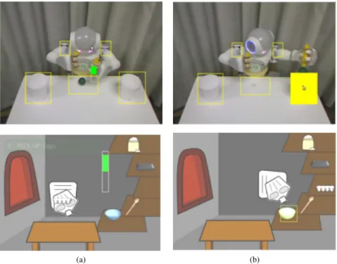
3.1 Screen-shots of our interface (Top row) and Sophie’s Kitchen (Bottom row). (a) shows positive reward given with a left click and drag up-wards; (b) shows guidance given with a right click on the object that

the teacher wants the agent to interact with. . . 22

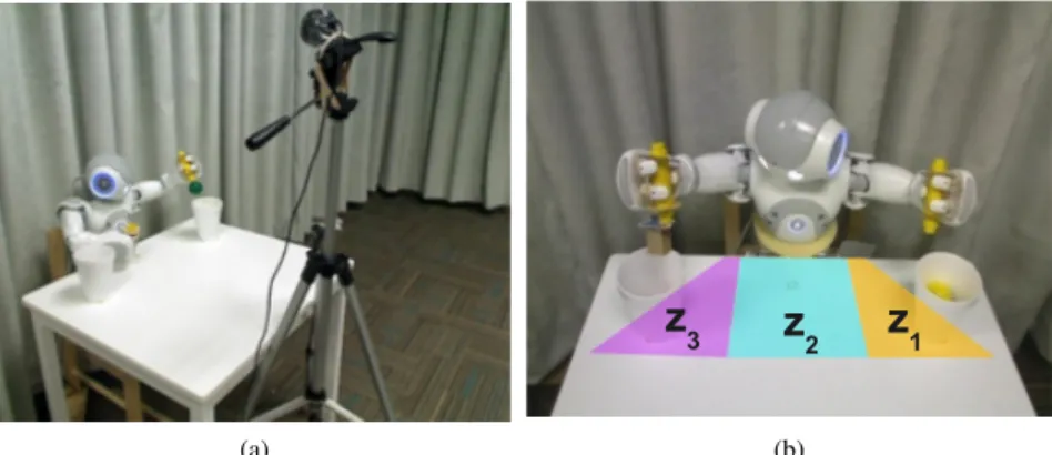
3.2 Experiment Setup. (a) Web camera captures the table and the robot for the user interface. (b) The table is divided in three zones. Orange, cyan blue and purple show z1, z2,andz3 respectively. The robot has an object at the tip of its right hand and is about to drop it in the right cup. . . 23

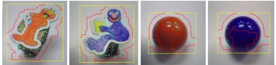
3.3 Images of different objects taken by robot’s camera. Light blue spots show SURF, red lines show the outline, and yellow rectangles show the bounding box or rectangle of interest of the object found. . . 26

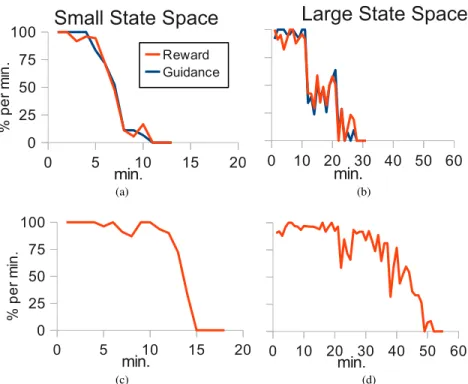
3.4 User interaction and training time with (a,b) and without (c,d) guidance input. Figures (a,c) and (b,d) show the results obtained in small and large state space respectively. The y-axis and legend are common for all graphs. . . 29

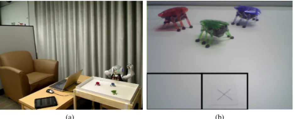
4.1 (a) Experimental setup, (b) View of the table from the Nao’s on-board camera. Sweep zone: bottom-left portion of the figure. Pick-up zone: bottom-center portion of the figure. Any other portion of the image is Wait zone. . . 39

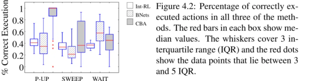
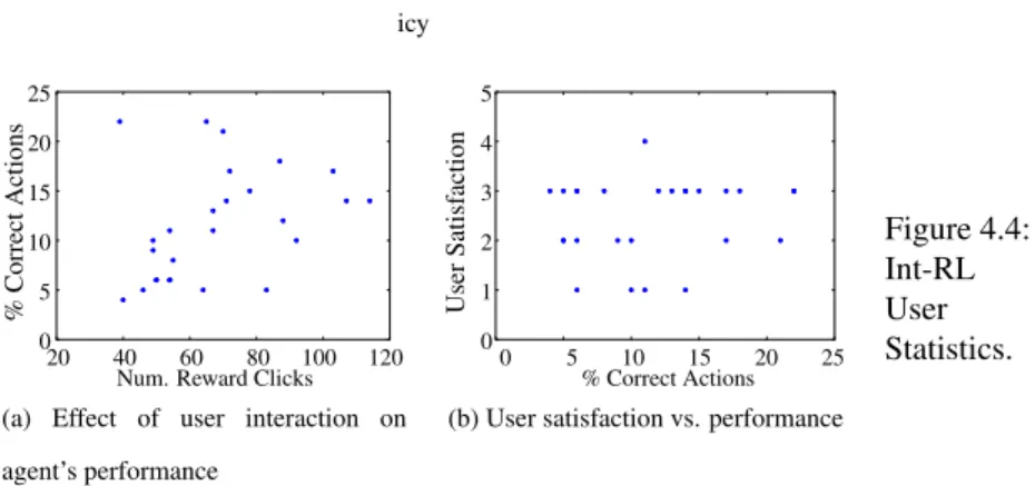
4.2 Percentage of correctly executed actions in all three of the methods. The red bars in each box show median values. The whiskers cover 3 interquartile range (IQR) and the red dots show the data points that lie between 3 and 5 IQR. . . 45

4.3 Example Int-RL Policies. . . 47

4.4 Int-RL User Statistics. . . 47

4.5 Examples of the networks demonstrated by the subjects. P-UP: Pick-Up, FBIPZ: Found a bug in Pick-Up Zone. Numbers in the end of the behaviors show their unique id numbers. . . 49

4.6 BNets User Statistics. . . 49

4.7 Example CBA Policies. . . 52

5.1 This diagram shows the distances and angles used to construct the 13 state variables used for learning with 3 keepers and 2 takers. Relevant objects are the 3 keepers (K) and the two takers (T), both ordered by

distance from the ball, and the center of the field. . . 62

5.2 This figure shows a screenshot of the visualizer used for the human to demonstrate a policy in 3 vs. 2 Keepaway. The human controls the keeper with the ball (shown as a hollow white circle) by telling the agent when, and to whom, to pass. When no input is received, the keeper with the ball executes theHoldaction, attempting to maintain possession of the ball. . . 64

5.3 This graph summarizes performance of Sarsa learning in Keepaway using four different algorithms. One demonstration of 20 episodes was used for all three HATlearners. Error bars show the standard error in the performance. . . 66

5.4 This graph summarizes performance of no prior learning and Proba-bilistic Policy Reuse learning using demonstrations from three differ-ent teachers. Each teacher performed demonstrations for 20 episodes. Error bars show the standard error in performance across 10 trials. . . 69

5.5 This graph summarizes performance of Probabilistic Policy Reuse lear-ning using five different demonstration sets. Error bars show the stan-dard error in performance across 10 trials. . . 71

5.6 This graph summarizes performance of Probabilistic Policy Reuse lear-ning using three sets of demonstrations from Subject B recorded under different simulator conditions: normal, fast and with limited actions. Each demonstration set consists of 20 episodes. Error bars show the standard error in performance across 10 trials. . . 73

6.1 Maze domain. The state-space consists of two continuous variables x, ythat define the horizontal and vertical location of the agent in the maze with reference to the lower-left corner. The agent starts from S and its goal is to navigate around the gray walls and reach the goal destination G. . . 83

6.2 Suboptimal demonstrations in the Maze domain. . . 83

6.3 Optimal path in the Maze domain. . . 84

6.4 Maze domain experiment results. . . 85

6.5 Mario domain experiment results. . . 88

6.6 Asymptotic performance of the DIS agent after 20,000 episodes in Mario AI. Here the performance is a function of the length of demons-trations (the number of state-action pairs recorded per demonstration). Each condition has 10 demonstrations. P-values obtained with two-samplet-tests between marked conditions for 10 trials. Values for the bar plot are the average of 10 trials. . . 92

6.7 Cumulative reward the DIS agent received during 20,000 episodes in Mario AI. Here the cumulative reward is a function of the length of demonstrations (the number of state-action pairs recorded per demons-tration). Each condition has 10 demonstrations. P-values obtained with two-samplet-tests between marked conditions for 10 trials. . . 92

Chapter 1

Introduction

Reinforcement Learning (RL), the problem of mapping situations to actions in order to maximize a reward signal [1], provides a convenient sequential decision making framework for conducting research on task learning. One of the major limitations of RL solutions is the high number of repetitions of observation and action selections a typical RL agent has to perform before the agent can reach a desired level of task performance. Slow learning performance and the difficulty of defining a reward function are major obstacles preventing practical use of RL solutions.

One of the main causes of the slow learning rates of RL algorithms, is the fact that the agents are assumed to have no prior knowledge of the task they are expected to solve. In this thesis, we show that learning from scratch is a limiting factor for the lear-ning performance of standard RL agents and that when prior knowledge is available, if the agent is provided means of leveraging this prior knowledge it can learn a task faster.

In RL problems the reward function can be thought of as a compact definition of the task. This reward function is often intuitive to define in most benchmarking domains. However, in the context of complex domains and real world problems, it may not be practical or feasible to define a task in advance as this may require a detailed knowledge of the state-space. This particular knowledge may be unavailable and hard-coding a

reward function may not be an option, or simply the definition of a task may change based on external requirements of users. In this thesis, we address this problem by implementing Inverse Reinforcement Learning for leveraging human demonstrations and computing a complementary reward function for an RL agent. We show that this secondary human reward function can be used for reward shaping for an RL agent to be able to fuse an environment reward signal with the learned reward signal.

The general theme of this thesis isReinforcement Learning from Demonstration: a combination of RL and Learning from Demonstration (RLfD). In a nutshell, we define RLfD as the class of agents that can leverage prior knowledge, specifically the prior knowledge obtained from an entity other than the agent itself, in an RL setting. In this thesis, we show that this class of agents have superior learning capabilities compared to off-the-shelf RL learners.

Augmenting the abilities of RL agents with prior knowledge is a relatively new topic of research within the field of RL. Design of RLfD agents is an underconstrained process. Some of the challenges are:

• Lack of infrastructure: Widely used RL algorithms are not equipped with

means for collecting priors about the task or possible solutions for the task.

• Source of prior:There are many possible sources for gathering prior knowledge

with varying consistency and quality; a previously trained RL agent, an online database for directing queries, a previously generated policy for a task and a human teacher can all be valid sources of prior knowledge.

• Use of prior: The structure in which the prior is conveyed to an RL agent is

crucial and it is not immediately clear how an agent can take advantage of this new input.

1.1

Contributions and Overview

In this thesis, we address all three of the challenges listed above. Our focus on obtaining the priors from humans and evaluating the use of human knowledge for RL agents in several ways. The overview of this thesis is as follows:

• In Chapter 2 we provide background material on Learning from Demonstration, the Reinforcement Learning problem, the Inverse Reinforcement Learning prob-lem and Reinforcement Learning from Demonstration, specifically by the means of Reward Shaping and Transfer Learning.

• In Chapter 3 we present a study of a previously introduced RL algorithm that al-lows a human demonstrator to provide online guidance and rewards to the agent. Our study is the first evaluation of this method in real-world robotic systems [2]. We show that guidance reduces the number of explored state and the learning time, and that its positive effects increase with state space size. In the presence of guidance the teacher reduces the number of interactions earlier in the training process and the teacher provides more positive rewards.

• In Chapter 4 we present our findings on a user study where na¨ıve teachers help a robot learn a task with three previously introduced learning from demonstration algorithms, one of which is the algorithm we evaluated with an expert teacher in the previous chapter. Here we evaluate the effect of human-agent interactions and present the results where we quantitatively and qualitatively compare the algorithms on a common real-world task [3].

• In Chapter 5 we show that it is possible to collect human demonstrations from teachers and use the teacher as an offline resource for modeling policies and for action selection advice. We contribute a novel RL algorithm Human-Agent Transfer (HAT) and evaluate the algorithm in a simulated soccer domain with three different teachers of varying skills [4]. We show that regardless of the skill level, human demonstrations can improve the asymptotic performance of an RL

agent.

• In Chapter 6 we introduce two novel RL algorithms, Static Inverse Reinforce-ment Learning Shaping (SIS) and Dynamic Inverse ReinforceReinforce-ment Learning Shaping (DIS) where human demonstrations serve as an offline resource for learning a secondary reward function [5] for reward shaping [6].We present two sets of experiments in a two dimensional Maze domain, and the 27 dimensional Mario AI domain. We compare the performance of our algorithms to previously introduced reinforcement learning from demonstration algorithms. Our exper-iments show that our approach outperforms the state-of-the-art in cumulative reward, learning rate and asymptotic performance.

Overall the contributions of this thesis show that in several simulated domains RLfD agents can surpass the abilities of RL agents. An RL agent can benefit from human priors in order to learn a task, improve its learning rate of a task, and it can do so by combining priors with its own experience.

Chapter 2

Background

This section provides background information on topics discussed throughout this the-sis. We organize the sub-sections to narratewhy we talk about the topic,what has been done in that field of research, and finallyhowprevious work relates to topics we present. We use a general-to-specific pattern with the hope to convey our deductive reasoning throughout this work.

2.1

Learning from Demonstration

In their book, Chernova and Thomaz define Robot Learning from Demonstrations as the field that explores techniques for learning a task policy from examples provided by a human teacher [7]. Algorithms for robot LfD seek to enable human users to expand the capabilities of robots through teaching instead of explicit programming. Specifically, LfD methods enable new robot behaviors to be learned based on demonstrations of the desired actions performed by the teacher. Many LfD algorithms are inspired by naturally occurring learning paradigms in humans and other animals, and the broad research goal is to develop an intuitive method of programming that is accessible to untrained, na¨ıve, users.

when one tries to understand where an approach stands within the field. Conveniently enough, one recent survey of the field presents a categorization of existing algorithms in order to help comparative assessments. In this survey Argall et al. [8] categorize then existing algorithms by:

• Demonstration Technique: teleoperation [9, 10, 11], shadowing [12, 13],

sen-sors on the teacher [14, 15, 16] or external observation [17, 18]; the categoriza-tion is dependent on who performs the task during demonstracategoriza-tion (the human or robot) and what information about the demonstrator’s actions is available.

• Policy Derivation Method: mapping functions (e.g., classification [9, 19, 20]

and regression [10] techniques), system model (e.g., reinforcement learning [21, 22]) and planning [23] approaches.

Previous work has proposed dozens of variants of learning from demonstration algo-rithms within each category mentioned above. However following three algoalgo-rithms are of specific interest to us, as we will see them being used later in Chapter 4: Interac-tive Reinforcement Learning [24], Behavior Networks [12, 25], and Confidence-Based Autonomy [9].

We introduce in detail and evaluate these three algorithms later in Chapter 4 in a comparative user study on a common real world task. We specifically chose these three algorithms because they are good representatives of the three different categories as presented by Argall et al. for (high level) task learning [8]. What we have learned from the implementation, and the na¨ıve users’ feedback on these different approaches influ-enced the algorithms we present in this thesis. Throughout our literature search and the user study we found that a complementary approach that would bring the positive aspects of multiple algorithms together can potentially improve teaching experience, learning efficiency, and the task performance.

2.2

Reinforcement Learning

Throughout this work we will frequently refer to concepts related to Reinforcement Learning, and that is why here we introduce a formal definition of Reinforcement Learning problems. We also talk about how previous work has used Learning from Demonstration within Reinforcement Learning framework, mainly as a way to convey prior knowledge to an agent.

Reinforcement learning (RL) is a common approach to agent learning from experi-ence. We define reinforcement learning using the standard notation of Markov decision processes (MDPs) [26, 27]. At every time step the agent observes its states∈Sas a vector ofkstate variables such thats=hx1, x2, . . . , xki. The agent selects an action

afrom the set of available actionsAat every time step, transitions into another state

s0and subsequently receives a rewardrbased on a reward functionR(s0). An MDP’s reward functionR:S×A7→Rand (stochastic) transition functionT :S×A7→S

fully describe the system’s dynamics. The agent will attempt to maximize the long-term reward delong-termined by the (initially unknown) reward and transition functions.

The agent chooses which action to take in a state via a policy,π:S 7→A. Policy

π(s)is modified by the agent over time to improve performance, which is defined as the expected total reward. Instead of learningπdirectly, many RL algorithms instead approximate the action-value function,Q:S×A7→_R, which maps state-action pairs to the expected real-valued return of an action chosen at a state. Value functionsV(s) quantify how valuable a given state is, and action-value functionsQ(s, a)describe how valuable is to take an action, at a given state. Depending on the RL approach, an agent may use eitherV orQto assess the potential return of a state, or an action.

In Chapter 5, we introduce (RL) agents that learn using Sarsa [28, 29], a well known but relatively simple temporal difference RL algorithm. Sarsa agents learn to estimate a state-action value functionQ(s, a). While some RL algorithms are more sample efficient than Sarsa (i.e. agents can reach to same task performance with less

experience), in Chapter 5 we will focus on Sarsa for the sake of clarity, as it is more likely that a wider audience would be familiar with Sarsa. We record demonstrations as temporal sequences oft state-action pairs{(s0, a0), ...,(st, at)}. However, these sequences typically only cover a small subset of all possible states in a domain. Typ-ically an RL agent’s goal is to generalize from the demonstrations and learn a policy

π : S 7→ A, coveringallstates that imitates the demonstrated behavior. Most sim-ilar to our approach in Chapter 5 is the work of Smart and Kaelbling, which shows that human demonstration can be used to bootstrap reinforcement learning in domains with sparse rewards by initializing theQ(s, a)(i.e. action-value function) using the observed states, actions and rewards [30]. In contrast to this approach, our work uses demonstration data to learn generalized rules, which are then used to bias the reinforce-ment learning process.

For RL agents, policies are as important as value functions sinceπdefines which action to take next. To clarify the connection between a policy and a value function, consider an agent that employs agreedy policywhich dictates the agent to takethe most valuable actionat a given states. An agent could use a policyargmax

a

Q(s, a)which would return the action that maximizesQ(s, a)for s. This is just a simple example, and when an agent usesV(s)instead ofQ(s, a)learning a more sophisticated policy

π(s)may be necessary instead of simply using a greedy policy [27]. Previous work proposed different algorithms for using demonstration data to learnπ. Deisenroth et al. present a survey on model-free and model-based policy search algorithms with a fo-cus on applications in robotics [31]. Fernandez et al. present Probabilistic Policy Reuse algorithm where an agent can exploit a previously learned policy in a new task. This work is at the intersection of policy learning with transfer learning. For the algorithm we present in Chapter 6, we suggest to use a human reward function recovered from demonstrations via Inverse Reinforcement Learning. We introduce Inverse Reinforce-ment Learning and Transfer Learning in the following sections of this chapter.

There is one big problem with LfD algorithms that RL can help. Typically, the final performance of LfD algorithms are inherently limited by the quality of the infor-mation provided by the human teacher. Most algorithms assume the dataset to contain high quality demonstrations performed by an expert. In reality, teacher demonstrations may be ambiguous, unsuccessful, or suboptimal in certain areas of the state space. A na¨ıvely learned policy will likely perform poorly in such areas [21]. To enable the agent to improve beyond the performance of the teacher, learning from demonstration may be combined with learning from experience, for which RL provides a theoreti-cally sound framework. In a recent work we investigated the use ofreward shaping

with LfD [32]. In RL, for reward shaping an agent sums one or more extra reward function(s) with the environment reward. In environments where the pre-coded reward function is sparse (e.g.r:= 0throughout the task andr:= 1when the agent reaches the goal), a shaping reward can provide data for a faster value approximation, which in turn can improve learning speed. In our approach, we allowed a demonstrator to make suboptimal demonstrations that lead to successful states. By using a shaping re-ward, their algorithm uses the demonstrations to speed up learning while dropping the requirement for the demonstrations to be given by an expert.

Just as RL algorithms can improve an LfD technique’s final performance, LfD al-gorithms possess a number of key strengths that can be beneficial for solving RL prob-lems. Most significantly, demonstration leverages the vast task knowledge of the hu-man teacher to speed up learning either by eliminating exploration entirely [33, 34], or by focusing learning on the most relevant areas of the state space [30]. Demonstration also provides an intuitive programming interface for humans, opening possibilities for policy development to na¨ıve teachers.

In robotics, RL approaches have enjoyed multiple past successes (e.g., inverted Helicopter control [35], and agent locomotion [36]). However they frequently take substantial amounts of data to learn a reasonable control policy. In many domains,

collecting such data may be slow, expensive, or infeasible, motivating the need for ways of making RL algorithms more sample-efficient.

2.3

Inverse Reinforcement Learning

Here we formally introduce the Inverse Reinforcement Learning (IRL) problem, and some commonly known solution techniques. IRL problem is also known as Inverse Optimal Control (IOC), or Inverse Optimal Planning (IOP) problem. We will use the name IRL in this thesis, and refer to IRL later in Chapter 6. Here we give details that motivate the use of IRL in our work.

We saw in the previous section that RL problems consist of learning a value func-tion, or a policy given a reward function. In contrast, IRL research deals with the problem of recovering a reward function (or a cost function) given an optimal policy and a state transition model (i.e. environment model). However, there are IRL algo-rithms that donotrequire the environment model to recover a reward function and we will refer to these as model-free IRL algorithms.

Even though the history of IOC goes back to Kalman’s question “When is a linear control system optimal?” [37], the number of publications show that in robotics and agents research the topic became more popular in early 2000’s. In an early paper, Ng and Russell base the motivation of IRL approaches to natural phenomena, stating that a reward function for humans’ and animals’ behavior control is often unknown [38]. For instance, for a bee that flies off to collect nectar, it is hard to know how the bee weights the relative benefit of flight distance against flight time, and risk from wind and predators in advance. Another similar example is human economic behavior. Therefore, it makes sense to try learn these relative weights based on observation of world states and executed actions. In his lecture notes Abbeel adds to this motivation a presupposition that a reward function also provides the most compact and transferable definition of a given task [39].

The general formal definition of an IRL problem is as follows: For a reward func-tion that consists of linear combinafunc-tions of a set of reward featuresR(s) =w>φ(s),

φ(s)is the vector of reward features that we compute based on the state vector, and

wis a vector feature weights. An IRL algorithm aims to find a set of optimal feature weightsw∗such that for all policies:w∗>µ(π∗)≥w∗>µ(π)(note thatµ(π) symbol-izes the expected cumulative sum of reward feature values (i.e. feature expectations) given a policyπ. Also,π∗is the optimal policy, whereasπis a suboptimal policy).

Some of the challenges for finding solutions to IRL problems are: the ambiguity of the solution (that is, more than one reward function may satisfy the constraints), the assumption that the expert demonstrations are optimal, and the assumption that we can enumerate all policies in order to compare one against another when finding an optimal set of reward features.

Abbeel divides existing IRL solution approaches into three main categories [39]: • Maximum Margin approach: Ratliff et al. introduce a margin functionm(π∗, π)

that returns an evaluation of disagreement between a given policy and the optimal policy, and aims to find a set of reward feature weights so that for all policies:

w>µ(π∗)≥w>µ(π) +m(π∗, π)[40, 41, 42].

• Feature Expectation Matching: Builds on the observation that for a policyπto be guaranteed to perform as well as the optimal policyπ∗, it is sufficient that the feature expectations match within a certain error threshold:

|w∗>µ(π)−w∗>µ(π∗)| ≤[22, 43, 44, 45].

• Reward Function as a Parameter: Assumes that an expert behaves according to a probabilistic policyπ(a|s, R, α), that is the expert’s policy is a function of the reward function. This formulation allows the use of Bayesian inference and evaluation of likelihood of a trajectory for a givenR, andα. Previous work then used various methods to find a reward function by sampling from this distribution and optimizing the likelihood of the policy [46, 47, 48].

Example applications of the IRL algorithms implemented in the work we cite above are simulated highway driving, aerial imagery based navigation, parking lot naviga-tion, destination prediction for urban naviganaviga-tion, human path planning, human goal inference, and quadruped robot locomotion.

All of the solutions we cite above are model based, where a transition model of the world – either deterministic, or probabilistic – is assumed to be known. Although outnumbered by model-based approaches , there are model-free IRL solutions that do notrequire an environment model. Klein et al. [49] approach the IRL problem as a supervised learning problem, where they suggest a two-layer approach. First layer consists of training a classifier to choose ascore function q(s, a)that evaluates the association of a state with an action, and the second layer learns a regressor to predict a rewardˆr=q(s, a)−γq(s0, a0), i.e. the difference between the past state-action score and the current state-action score.

Boularias et al. also introduce Relative Entropy Inverse Reinforcement Learning (RE-IRL), a model-free IRL algorithm [5]. RE-IRL aims to minimize the KL - diver-gence between two probability distributions: a conditional distributionP(τ|w), and a user-defined distributionQ(τ), whereτ=h(s0, a0), . . . ,(sH, aH)iis a demonstrated trajectory of lengthH, andwis the vector of reward feature weights. The distribu-tionQcan be defined so that samples from a particular part of the trajectory space are weighted with more importance than others. If we want to recover the most informative reward feature weights then we can chooseQ(τ)to be a uniform distribution across the trajectory space. Boularias et al. [5] define the RE-IRL problem as:

max w g(w) =w >_fπE_{−lnZ(w)−λkwk} 1 Z(w) = ΣτQ(τ) exp(w>fiτ) P(τ|w) = 1 Z(w)Q(τ) exp(w >_fτ i)

For finding the vector of reward feature weights that maximize the objective function

g(w), the algorithm empirically estimates the subgradient of the objective function with importance sampling of trajectories and executes gradient ascent.

Boularias et al. evaluate the algorithm on a simulated robot for ball-in-a-cup task, based on human expert demonstrations where a human tries to catch a ball attached to a string hanging off the bottom of a cup [5]. Muelling et al. used RE-IRL for inferring strategies for table tennis based on human gameplay tracking data [50]. They show that the estimated reward function was able to capture strategic information enough to distinguish the expert among players with different skill levels and styles.

In Chapter 6 we use RE-IRL algorithm as an off-the-shelf solution for recovering a reward function from demonstration data. We do not intend to improve RE-IRL nor do we plan to go in the direction of IRL research. The requirement of the algorithms we present is to employ a simple to implement, yet usable, model-free IRL algorithm that can recover a function that would help a learner assess how desirable is a change in the world state. Using relative weights of reward features, we execute gradient ascent in order to reach a goal state on a path that prioritizes the relative importance of the features along the path (e.g. approach in x direction can be more desirable than approach in y direction).

2.4

Transfer Learning

Transfer Learning (TL) allows an agent to begin learning with an informative prior instead of relying on random exploration [51]. The intuition behind TL is that general-ization may occur not only within tasks, but alsoacross tasks.

In Chapter 5 we introduce Human-Agent TransferHATalgorithm. ForHAT, we use Rule Transfer[52], a particularly appropriate transfer method that is agnostic to the knowledge representation of the source learner. The ability to transfer knowledge be-tween agents that have different state representations and/or actions is a critical ability

when considering transfer of knowledge between a human and an agent. The following steps summarize Rule Transfer:

1a: Learn a policy (π : S 7→ A) in the source task. Any type of reinforcement

learning algorithm may be used.

1b: Generate samples from the learned policyAfter training has finished, or during

the final training episodes, the agent records some number of interactions with the environment in the form of(S, A)pairs while following the learned policy.

2: Learn a decision list (Ds : S 7→ A) that summarizes the source policy. After

the data is collected, a propositional rule learner is used to summarize the col-lected data to approximate the learned policy by mapping states to actions.1 _This

decision list is used as a type of inter-lingua, allowing the following step to be independent of the type of policy learned (step 1a).

3: Use Dt to bootstrap learning of an improved policy in the target task. For

instance, previous work [52] provided three ways of leveraging this knowledge; we discuss two of these methods later in Chapter 5.

Transfer learning methods for reinforcement learning can transfer a variety of infor-mation between agents. However, many transfer methods restrict what type of learning algorithm is used by both agents (for instance, some methods require temporal differ-ence learning [53] or a particular function approximator [54] to be used in both agents). However, when transferring from a human, it is impossible to copy a human’s “value function” — both because the human would likely be incapable of providing a com-plete and consistent value function, and because the human would quickly grow wary of evaluating a large number of state-action pairs.

1_{Additionally, if the agents in the source and target task use different state representations or have}

differ-ent available actions, the decision list can be translated via inter-task mappings [52, 53] (as step 2b). For our work, this translation is not necessary, as the source and target agents operate in the same task.

In a recent work by Knox and Stone [55], theirTAMER[56] system learns to predict and maximize a reward that is interactively provided by a human. The learned human reward is combined in various ways with Sarsa(λ), providing significant improvements. The primary difference betweenHATand this method is that we focus on leveraging human demonstration, rather than estimating and integrating a human reinforcement signal.

The idea of transfer between a human and an agent is somewhat similar toimplicit imitation[57], in that one agent teaches another how to act in a task, butHATdoes not require the agents to have the same (or very similar) representations.

Allowing for such shifts in representation gives additional flexibility to an agent de-signer; past experience may be transferred rather than discarded if a new representation is desired. Representation transfer is similar in spirit toHATin that both the teacher and the learner function in the same task, but very different techniques are used since the human’s “value function” cannot be directly examined.

High-level adviceand suggestions have also been used to bias agent learning. Such advice can provide a powerful learning tool that speeds up learning by biasing the be-havior of an agent and reducing the policy search space. However, existing methods typically require either a significant user sophistication (e.g., the human must use a specific programming language to provide advice [58]) or significant effort is needed to design a human interface (e.g., the learning agent must have natural language pro-cessing abilities [59]). Allowing a teacher to demonstrate behaviors is preferable in domains where demonstrating a policy is a more natural interaction than providing such high-level advice.

2.5

Reward Shaping

Reward shaping, derived from behavioral psychology [60], is a way of incorporating prior knowledge in the learning process. A shaping rewardF provides an agent with

additional information after each state transition. With shaping rewards, an agent is rewarded for taking appropriate steps toward the goal. This extra reward supplements the environment reward which is typically defined as a sparse function for practical reasons.

The extra reward signalF, defined by agent designers, is added to the environment rewardR, defined by problem designers. The agent learns a task using the shaped rewardR0:

R0(s, a, s0) =R(s, a, s0) +F(s, a, s0) (2.1)

F function usually encodes heuristic knowledge, and is intended to complement the typically less informative signalR. As we mentioned earlier, the agent’s goal is defined by the reward function, and by manipulating the reward signal we may risk changing the task. Ng et al. [61] proved that potential-based shaping is a sound way to provide a shaping reward without changing the reinforcement learning problem.

2.6

Reinforcement Learning from Demonstration

RL from Demonstration (RLfD) is a learning setting for RL agents where both de-monstrations and an environment reward signal are available. Algorithms use different methods to convert demonstrations into a representation that the agent will be able to use as heuristic information and the environment reward is treated as the ground truth for learning. Early work on Reinforcement Learning from Demonstration (RLfD) was presented by Schaal [62], in which the term described a set of approaches that lever-aged initial training for learning a policy and a value function from demonstrations, followed by a “trial by trial learning” with RL.

Most recently, Brys et al. introduced a new algorithm we refer to as Similarity Based Shaping (SBS) [32]. With the SBS algorithm Brys et al. took a different ap-proach to investigate the use of prior knowledge as a potential-based shaping reward.

The SBS algorithm uses human demonstrations as a potential functionΦD(s, a)for potential-based shaping. With this approach each demonstrated state-action pair is as-sumed to be desirable for the agent, and using a similarity metric, the SBS algorithm computes a shaping rewardF. During learning, the agent receives a shaped reward sig-nalR0=R+Fwhich is the combination of the environment reward (i.e. ground truth) and the shaping reward. The SBS algorithm uses non-normalized multi-variate Gaus-sian distributions to compute the similarity between demonstrated states and observed states throughout learning.

Chapter 3

Effect of Human Guidance and

State Space Size on

Interactive Reinforcement

Learning

In this chapter, we study how Reinforcement Learning can be made more efficient for real-world robotic systems by enabling human teachers to provide feedback at run-time. Our feedback differs from the related work in the sense that the teacher can provide not only reward for the preceding action but also guidance for the subsequent action. Our work builds upon a series of studies by Thomaz et al. that show that in a reinforcement learning scenario users tend to not only reward past actions but also provide anticipatory rewards to guide the learner in future actions [63]. Based on this analysis, Thomaz and Breazeal presentInteractive Reinforcement Learning(Interactive RL), an algorithm that enables a human trainer to 1) provide positive and negative rewards in real time in response to robot actions, and 2) provide anticipatory guidance input that restricts action selection choice and guides the learner towards performing the desired behavior [24]. The authors show that incorporating user guidance into the policy learning process significantly improves the learning rate of a software agent by reducing the number of states it explores.

We report the results of a case study in which Interactive Reinforcement Learning was applied to teaching an Aldebaran Nao robot. To our knowledge, this work is the first to apply this type of learning algorithm to a real-world robotic system. To evaluate the approach, we closely reproduce the interactive reward interface proposed in [24] and perform four experiments comparing Interactive RL with and without anticipatory guidance for two different state space sizes. We discuss modifications made to apply this learning approach to a real-world system. Our results show that guidance signif-icantly reduces the learning rate, and that its positive effects increase with state space size. We conclude with a discussion of the benefits and challenges of using Interactive Reinforcement Learning in real-world robotic applications.

3.1

Overview

The ability to acquire and customize robot behavior through learning is vital for the successful deployment of robots in a broad range of consumer and service applications. In order for robots to become effective assistants in diverse human environments we must develop the capability to quickly and efficiently customize robot behavior and learn new tasks. Numerous works have addressed the challenges of learning in complex real-world environments [64, 65]. One popular technique is Reinforcement Learning (RL) [66], which enables a robot to learn from rewards it obtains while attempting to perform its task. Although RL algorithms have had great success in offline learning and software applications, the large amount of data and high exploration times that such algorithms require make them intractable for many real-world robotic domains.

A number of recent work has shown that in the presence of a human, robotic sys-tems can be designed to take advantage of human input [67, 9]. In the case of Rein-forcement Learning, one example is the work of Kaplan et al. where they present a technique in which user-generated reward and punishment signals are used to train the robot new tasks in a form of clicker training [68]. Another related work was presented

by Smart and Kaelbling, where human demonstrations of robot actions can be used to make learning of otherwise intractable policies possible [11]. Also, Knox and Stone introduce the TAMER framework that allows a human trainer to interactively shape an agents policy via reinforcement signals [69].

The motivation behind our work is similar to these past examples.

3.2

Description of Interactive RL Algorithm

The Interactive Reinforcement Learning algorithm with human guidance, as described in [24], modifies traditional Q-learning by integrating human input into the reward and action selection mechanisms. In Interactive RL, allreward input to the robot comes from the human teacher instead of the environment; the teacher is given a short pe-riod of time following each action to provide positive or negative feedback. Addition-ally, during a short delay period between actions, the user can provideguidance input. Guidance is given with respect to an object or location (e.g., table), with the effect of restricting the choice of immediately available actions to those related to the target ob-ject (e.g., look at table, put down obob-ject on table). This technique can be thought of as a means of directing the robot’s attention to the target object or area. In the following sections, we first present the details of the Interactive RL algorithm and then describe the interaction interface used by the human teacher.

Algorithm 1 presents the pseudo-code for Interactive RL. The algorithm extends traditional Q-learning with the addition of human reward input (lines 18-21) and human guidance (lines 6-8). When learning begins, the agent has no knowledge of the task and the Q-table contains only the robot’s current state. The table expands (line 17) as the robot performs actions, receives rewards and encounters new states, and the Q-values are updated (lines 23-24). In our implementation, we set the learning rateα= 0.3and the discount factorγ = 0.75. We initialize the Q-values for every new state that the agent discovers to0.5.

Our initial implementation of Interactive RL followed the exact description pro-vided in [24]. Following preliminary testing, we implemented a change to the ac-tion selecac-tion mechanism. Specifically, in the original implementaac-tion, in the absence of teacher guidance the agent uses theQ[s, a]values to weight available actions and probabilistically select the next action to perform. During preliminary experiments, we found that this approach resulted in very long learning times for the robot (over 80 minutes for the small domain described in Section 3.3.2). In followup experiments, we found thatε-greedy action selection (lines 1-2, 12-15) results in significantly improved learning times. In this selection method, the robot performs the optimal action with probability1−εand a random action with probabilityε. Over time, the value ofε de-cays (line 25) until eventually the robot always performs the optimal action (i.e., policy exploitation).

Theε-greedy action selection method is used to select the next action both when a guidance signal is present and when it is absent. If none of the actions specified by the guidance message are valid (not physically possible), the robot ignores the guidance message and usesε-greedy selection to pick among all available actions. For example, in the domain described in Section 3.3.1, thePickUpaction is not valid before the robot determines whether there is an object in front of it using theTakePictureaction.

A key contribution of the original Interactive RL paper is the interactive reward interface that enables an online user to train a virtual robot to bake a cake in a domain called Sophie’s Kitchen1_{. The human trainer uses the left mouse button to provide}

reward signalsr= [−1,1]for the agent’s actions, and the right mouse button to provide guidance for future actions. In this work, we recreate the interactive reward interface for a real robot by providing the human trainer with a fixed view of the environment via a web-cam (Figure 3.2a). As with the algorithm, we began by implementing the interface described in [24] in order to evaluate its use in real-world systems. Following

1_{The original Sophie’s Kitchen web application is available at}

(a) (b)

Figure 3.1: Screen-shots of our interface (Top row) and Sophie’s Kitchen (Bottom row). (a) shows positive reward given with a left click and drag upwards; (b) shows guidance given with a right click on the object that the teacher wants the agent to interact with. preliminary evaluations we found the need to make one modification to the interface in order to improve the ease of interaction for our domain.

In our evaluation, the reward interface functions as in the original web application, in which left clicking anywhere in the image brings up a reward bar (Figure 3.1a) that the user can fill with a positive or negative reward value representing the desirability of the current state. The guidance interface differs slightly; instead of allowing the user to click anywhere, our interface highlights five rectangular regions as potential guidance targets. The teacher provides guidance by right-clicking within the highlighted boxes (Figure 3.1b). Table 3.1 lists the five regions and their effect on action selection.

(a)

z

z

z

(b)

Figure 3.2: Experiment Setup. (a) Web camera captures the table and the robot for the user interface. (b) The table is divided in three zones. Orange, cyan blue and purple showz1, z2,andz3respectively. The robot has an object at the tip of its right hand and

is about to drop it in the right cup.

3.3

Experimental Setup

To investigate the ways in which human guidance impacts the policy learning rate in real-world systems we developed an object sorting domain using an Aldebaran Nao humanoid robot. The domain setup consists of a stationary work table where the Nao is seated on a chair. Magnetic objects are placed in front of the robot one at a time. The robot must learn to use its camera at the appropriate time to identify the characteristics of the object and then to pick up and place the object in one of two cups located on the table. The user observes the robot’s actions via a web-cam (see Figure 3.2a) and provides feedback to the robot through the graphical user interface. The described setup enables us to evaluate the impact that human guidance input has on robot learning performance and the usability of the user interface.

3.3.1

Domain

The experimental domainD = (Z, S, A, T)is defined by a finite set of zonesZ, a finite number of world statesS, a finite set of possible robot actionsAand the transition functionT :S×A→Sthat determines transitions between states by way of actions.

ZonesZrepresent the regions where the robot’s arms or an object can be located. In our domain,Z ={z1, z2, z3}corresponds to the left, front and right side of the robot

respectively (Fig. 3.2b).

The state of the world S = {Sr∪So} consists of the union of the state of the robotSr and state of the object being classified So. The robot state is defined by

Sr= (zlh, zrh, hando), wherezlh, zrh∈Zcorrespond to the current zone of the left and right hands, respectively, andhando∈ {lef t, right, none}represents whether an object is located in either of the robot’s hands, or not. For example, in Fig. 3.2b the robot’s state is represented bySr= (z1, z3, right).

The object state is defined bySo= (I, oz, op), whereIis an object descriptor that specifies the characteristics of the object using a set of features described in Section 3.3.2. oz ∈ Z is the current zone of the object, andop ∈ P is the placement of the object such thatP ={z1, z2, z3, right cup, lef t cup}. For example, in Fig. 3.2b the

object state is represented bySo= (pattern, z3, z3).

The robot has eleven possible actions,T akeP icture,xP ickU p,xP utDown,xDrop,

xLef t, andxRightwherex∈ {L, R} determines the arm with which the action is performed. TheT akeP ictureaction makes the robot take a snapshot of the table in front of it and extract features from the image to determine the characteristics of the ob-ject currently placed there (if any) (see Fig. 3.3).xRightandxLef tactions move the hands between zones (e.g. LLef tmoves left hand left, that is, to Zone 1 andRLef t

moves right hand left, that is, Zone 2. Note that the robot’s left hand can operate only inz1,2, and the right hand can operate only inz2,3, which enables the robot to pick

up an object with either hand but allows only one hand to reach each cup andDrop

the object into it. If the robot initially picks up the object with the wrong hand, it can switch hands by performing axP utDownaction followed by axP ickU p.

Table 3.1 shows how different guidance messages restrict the set of available robot actions. Note that the degree to which guidance reduces the set of actions has a

signif-Guidance ActionSet

Zone 1 LLef t,LDrop

Zone 2 LP utDown, LP ickU p, RP utDown,

RP ickU p,T akeP icture

Zone 3 RRight,RDrop

Left Shoulder LP ickU p, LRight, LLef t,

LP utDown,LDrop

Right Shoulder RP ickU p, RRight, RLef t,

RP utDown,RDrop

Table 3.1: Guidance messages restrict action selection to the set of available actions as shown. The first letterLandRdenotes either Left or Right hand depending on the hand with which the action is executed.

icant effect on the learning rate. If guidance does not significantly reduce the choice of available actions, then the effect of this input method is reduced since the robot will have to choose randomly among them. In contrast, if the guidance message limits the robot to a single action, then all choice is taken away from the robot; this approach would be equivalent to the human demonstration techniques applied inlearning from demonstrationapproaches [70, 11]. The effect on learning would be to eliminate ex-ploration, resulting in a policy that is only as good as the decisions demonstrated by the human, and is poorly defined in areas of the state space not encountered during training. Further studies are needed to determine the precise impact of these choices. In our implementation we chose to design guidance as an effective teaching method that always restricts the list of available actions but never reduces action selection to a single choice.

3.3.2

Experimental Conditions

We performed four sets of experiments to evaluate the Interactive RL algorithm and study the effects that 1) teacher guidance, and 2) size of the state space have on learning performance. The same object sorting task was used for all experimental conditions. In the no-guidance condition, the user was restricted to only the reward input, and the

Figure 3.3: Images of different objects taken by robot’s camera. Light blue spots show SURF, red lines show the outline, and yellow rectangles show the bounding box or rectangle of interest of the object found.

guidance condition allowed for both types of input. To vary the state space size we changed the number of features used to describe the object being sorted. Specifically we used the following two experimental conditions:

• Small deterministic state space: In the small state space condition, the object

descriptorI ofSo = (I, oz, op)consists of a single variable with two possible values,plainorpattern, representing the color class of object. This mapping is determined based on the number of Speeded Up Robust Features (SURF) [71] identified in the image of the object and identifies the object as either a solid colored ball or a character magnet, respectively. Specifically, objects for which over 50 SURF features were identified were characterized aspattern, otherwise the object wasplain. In our tests we found that the number of SURF features deterministically separate these two object types. Combining this binary object representation with other state information, such as object location and robot state, results in 360 possible states.

• Large, non-deterministic state space:In the large state space condition, the

ob-ject descriptorIconsists of four elements, where measured values are rounded to the closest defined category: the number of SURF features (50, 100, or 150), smoothness (0.05 or 0.1), entropy (5.0 or 10.0) and area of the bounding box of the object (15,000, 20,000 or 25,000). We calculate smoothness and entropy as described in [72]. After image processing, the value for each descriptive

fea-ture is thresholded into the categories listed above. This representation was pur-posefully designed to reduce the size of the state space by providing a small set of possible values for each variable, while at the same time making sure that none of the descriptive elements alone is sufficient for distinguishing between the plain and patterned object types. For example, although they are the same type of object, the plain green and plain yellow magnets have different smoothness, perceived area and entropy states. To the robot these objects therefore appear distinct and it must learn that they belong to the same group. Furthermore, this representation is non-deterministic and variations in object placement will result in slightly different state representations, allowing us to evaluate how Interactive RL performs under these conditions. In total, the large state space representation results in 6480 states.

During the experiments all processing was performed on a PC connected to the robot over the network. For image processing we used OpenCV [73], examples of the processed images are shown in Figure 3.3. All experiments were performed by author of this thesis. The teacher used the following consistent guidance and reward shaping protocol. For the first 20 actions of the experiments, all actions were given reward and guidance (in case of experiments with guidance). After 20 actions, reward and guidance were given only after the incorrect action that the robot performed. After each incorrect action, the following 5 actions were rewarded and guided. If the action was correct, no reward or guidance was given until the next incorrect action. In the small state space condition we usedε= 0.1andδε= 0.002(εreaches 0 after 50 time steps), and in the large state space conditionε= 0.1andδε= 0.001(ε= 0.1reaches 0 after 100 time steps). We terminate learning once the robot is able to correctly sort three objects into each cup without guidance or reward. Objects were presented to the robot in random order. A video of the experiment and the interface can be found

online2_.

3.4

Results

We ran three trials for each of the four experimental conditions, the averaged results are presented in Figure 3.4. Graphs plot the level of teacher involvement over time in terms of the percentage of actions for which the teacher provided reward and/or guidance. A summary of experimental statistics is given in Table 3.2.

A comparison of plots Fig. 3.4a to 3.4c and Fig. 3.4b to 3.4d, shows that the use of guidance remarkably reduces the learning time (small state space: 28%, large state space:44%) as well as the number of states explored (small state space:51.5%, large state space: 38%). In effect, the robot learns more quickly with guidance because it selects the correct action more frequently and therefore avoids exploring irrelevant areas of the state space. As a result, we observe that in the presence of guidance the teacher reduces the number of interactions earlier in the training process compared to the no-guidance condition.

We also observe differences in teacher behavior between the guidance and no-guidance conditions. The cumulative reward for the trials is positive in the presence of guidance and negative in its absence. This is a direct consequence of the fact that the robot selects more inappropriate actions when learning without guidance and the teacher spends more time giving praise to the robot than punishment. This is an inter-esting result given that a number of studies show that given the option between reward and punishment most human teachers prefer to use positive reward and avoid punish-ment when training an agent [63].

In summary, the comparison study shows that teacher guidance significantly re-duces learning time by reducing the number of states explored. This result supports the findings of [63], in which average reductions of30%in case of expert teachers and49%

0 5 10 15 20 0 25 50 75 100

min.

Small State Space

min.

Large State Space

(b) 0 5 10 15 20 0 25 50 75 100

min.

min.

Figure 3.4: User interaction and training time with (a,b) and without (c,d) guidance input. Figures (a,c) and (b,d) show the results obtained in small and large state space respectively. The y-axis and legend are common for all graphs.

in case of non-expert teachers were observed in the number of trials. Furthermore, we find that the impact of teacher guidance increases as the size of the state space grows. We hypothesize that similar benefits would be observed with respect to growth in the size of the action space, although further studies are required to verify this effect.

3.5

Discussion

The Interactive Reinforcement Learning approach has several key strengths: 1) its sim-ple action selection mechanism can be integrated into a broad range of existing RL approaches, 2) its application results in a flexible learning system that can learn inde-pendently but is able to take advantage of human guidance when it is available, and 3) guidance is combined with independent exploration in a way that enables the robot

Fig.3.4a Fig.3.4b Fig.3.4c Fig.3.4d #States 11.33 42.67 22 68.67 #Actions 82 201 134.67 366.67 Cumul. Rew. 16.67 58 -44.67 -74.67 Total #G. 44 113.67 0 0 Training Time [min.] 14 31 18 55

Table 3.2: Experiment statistics. All results are shown as the average of three trials for each experiment. Number of states discovered (#States), total number of actions performed (#Actions), sum of the positive and negative rewards given (Cumul. Rew.), total number of guidance given (Total #G.) and training time.

to not only imitate the demonstrated behavior but also to surpass the performance of the teacher if necessary.

However, there are a number of challenges to deploying this approach in real-world applications. The current implementation of the teaching interface assumes a fixed-camera setup that enables the human user to select relevant areas of the state space for guidance. While this interface may translate into some service and factory applications, it is not suitable for mobile robotic systems or unconstrained environments. Further work is required to evaluate how other input methods, such as portable tablets, speech, and gestures, can be used to interact with the robot in this setting.

The running time of the algorithm is another area for potential improvement. Cur-rently, the robot requires approximately half an hour to learn a relatively simple task. Much of this learning time is dependent on the time required to execute each action. For example, an average of 201 actions was required to learn the large task, which is a relatively small number compared to the total number of states in the domain, but each action had an average time of 9.8 seconds. Other critical factors include the explo-ration rate, state representation, and the degree to which guidance reduces the choice of available actions. In order to enable this approach to scale to more complex domains, we must explore the effects that these factors have on learning time, as well as study how Interactive RL can be applied to RL algorithms that utilize continuous state space representations which model complex world state more effectively [74, 75]. An

inter-esting future work is a comparison of the Interactive RL algorithm with the TAMER framework [56] and the SABL algorithm [76]. The TAMER framework learns a human reward function however does not contain any guidance input. The SABL algorithm is able to interpret the lack of feedback which is different from both the Interative RL and the TAMER algorithms. A fair comparison of these three RL algorithms that learn tasks from humans can be informative for discovering future directions for developing more capable and efficient algorithms.

We compared two conditions, the large state space, in which the generalization across multiple sensory inputs had to be learned, and the small state space, in which a single sensory input automatically generalized across the two object types. Both con-ditions were designed through manual selection of the appropriate state features in a preliminary testing stage. In the case of the small state space, the chosen representa-tion enabled us to teach the task more effectively because instructing the robot through the use of just one to two patterned magnets enabled it to automatically generalize the behavior to all patterned shapes. In the case of the large domain, each patterned item was described by a unique set of features, and more examples were required for the algorithm to learn the appropriate generalization. The large state space more closely represents a real-world scenario; robots designed for operation in real-world environ-ments in the presence of non-expert users are likely to have an even larger number of sensory inputs, possibly with many irrelevant features, which will lead to longer lear-ning times. This motivates the need for semi-autonomous feature selection methods that reduce the size of the state space and enable the robot to learn more effectively.

Finally, when designing interactive learning algorithms we must consider their us-ability for non-expert users. This chapter focused on empirical evaluation of the best-case scenario in which the robot was taught by a roboticist after numerous practice trials.

Algorithm 1Interactive Q-Learning with human generated reward and guidance

1: ε= initial value

2: δε=ε/ number of desired time steps to stop exploration

3: Initialize Q-table with starting state

4: whilelearningdo

5: whilewaiting for guidancedo

6: ifreceive human guidancethen 7: g=guidanceT arget

8: end if

9: end while

10: ifreceived guidancethen

11: A= set of legal actions that only containg

12: else

13: A= set of legal actions for the current state

14: end if

15: rand= random number [0,1]

16: ifrand > εthen 17: a=arg maxaQ[s, a]

18: else

19: a= randomly selected action inA

20: end if

21: executeaand transition tos0

22: ifs0not in Qthen 23: adds0to Q-table

24: end if

25: whilewaiting for rewarddo

26: ifreceive human rewardthen 27: r= human given reward

28: else 29: r= 0 30: end if 31: end while 32: update values: Q[s, a]←Q[s, a] +α(r+γ(maxa0Q[s0, a0])−Q[s, a]) 33: ifε >0then 34: ε←ε−δε 35: end if 36: end while

Chapter 4

A Comparison of Three

Learning from Demonstration

Algorithms

In the previous chapter we studied how Reinforcement Learning can be made more ef-ficient for real-world robotic systems, however our study was evaluated using an expert teacher’s demonstrators. In this chapter, we present findings from a user study in which we asked non-expert users to use and evaluate three different robot Learning from De-monstration algorithms. The three algorithms we chose – Behavior Networks, Inter-active Reinforcement Learning, and Confidence Based Autonomy – utilize distinctly different policy learning and demonstration approaches. This enables us to examine a broad spectrum of the field.

4.1

Overview

Research on robot Learning from Demonstration has seen significant growth in recent years, but the field has had only limited evaluation of existing algorithms with respect to algorithm usability by na¨ıve users. Despite the existence of a diverse body of work, research in Learning from Demonstration lacks a comparative user study that focuses