Multidimensional Mastery Testing with CAT
A THESIS
SUBMITTED TO THE FACULTY OF THE GRADUATE SCHOOL OF THE UNIVERSITY OF MINNESOTA
BY
Steven Warren Nydick
IN PARTIAL FULFILLMENT OF THE REQUIREMENTS FOR THE DEGREE OF
DOCTOR OF PHILOSOPHY
Niels Waller Thesis Advisor
c
Steven Warren Nydick 2013
Acknowledgements
This dissertation reflects more than a simple study expanded over more than 200 pages. This paper represents who I am but also how I have grown over the course of my studies, as a student, a scholar, a friend, and a collaborator. Many people have earned my gratitude for their contribution to my time in graduate school. The following is only an incomplete list of those I have met along the way.
To my advisor, Niels Waller, who pushed me to be a better writer and scholar, helped me when needed, and allowed me to explore my own interests.
To my colleague and committee member, Chun Wang, who had faith in my research and writing abilities and helped me accomplish more professionally in the little time that I have known her than I had in the rest of my graduate studies.
To my committee members, David Weiss and Sandy Weisberg, who (as advisors of mine at one time in graduate school) have supported my studies and provided encour-aging words and more than enough time and flexibility over the years.
To my undergraduate mentor, Benjamin Lovett, who had faith in my abilities and helped me discover my own path in graduate school. More than anyone else, he improved my writing ability through detailed and thoughtful criticism.
To the Psychology Department staff, especially Lynn Burchett and Judy Peterson, who assisted with all of the necessary administrative tasks, pushed me to hand in all
one PhD.
To my network of supportive friends, Caren Arbeit, Mayumi Baker, Ben Babcock, Peter Marks, Stefani Quam, Hannah Riederer, and Shelby Vanderberg, who provided many ears (and drinks) over the years to help me express many of the frustrations of graduate school and escape from those frustrations.
To my colleagues on the sixth floor of Elliot Hall, Ben Babcock, Leah Feuerstahler, Rick Geyer, Chris Hulme-Lowe, Jieun Lee, Chaitali Phadke, and Dong Seo, who helped me think through problems and discussed the many intricacies of psychometrics that no one else would discuss.
To my colleagues at the American Registry of Radiologic Technologists and my co-interns at ACT, who provided me with projects that inspired fruitful ideas (including those that led to my dissertation) and challenged me to apply my abstract knowledge to practical problems.
To Jeff Jones, who always listened to my incredibly long rants, usually followed by beer, a bucket of hot wings, and a British comedy, and helped edit (and shorten) everything that I wrote in graduate school.
To my father, sister, and the rest of my family, who have always supported and encouraged me through the endless years of school and probably assumed that I would stay in graduate school at least three lifetimes into the future.
To my wonderful girlfriend, Lian Hortensius, who, according to friends, has made me smile much more than I did in the past.
To my mom. I love you and miss you.
Abstract
Computerized mastery testing (CMT) is a subset of computerized adaptive testing (CAT) with the intent of assigning examinees to one of two, mutually exclusive, cat-egories. Most mastery testing algorithms have been designed to classify examinees on either side of a cut-point in one dimension, but many psychological attributes are inher-ently multidimensional. Little psychometric work has generalized these unidimensional algorithms to multidimensional traits. When classifying examinees in multidimensional space, practitioners must choose a cut-point function that separates a mastery region from a non-mastery region. The possible cut-point functions include one in which a lin-ear combination of ability across dimensions must exceed a threshold and one in which each ability must exceed a threshold irrespective of any other ability. Moreover, two major components of every classification test are choosing successive questions and de-termining when a classification decision should be made. One frequently used stopping rule in unidimensional mastery testing is the Sequential Probability Ratio Test (SPRT), in which a classification is made either when the log-likelihood test statistic is sufficiently large or when the maximum number of items has been reached. Due to inefficiencies in the SPRT, alternative algorithms have been proposed, such as the Generalized Likeli-hood Ratio (GLR), and the SPRT with Stochastic Curtailment (SCSPRT). The current study explores properties of unidimensional classification testing algorithms, generalizes unidimensional methods to multidimensional mastery tests, and then tests many of the multidimensional procedures. Most of the multidimensional algorithms yield relatively efficient and accurate multidimensional classifications. However, some multidimensional classification problems, such as classifying examinees with respect to a linear classifi-cation bound function, are more robust to poor choices in the item bank or adaptive
study is proposed to better combine sequential classification methods with those based on directly quantifying incorrect classifications. I conclude by discussing consequences of the results for practitioners in realistic mastery testing situations.
Contents
Acknowledgements i
Abstract iii
List of Tables ix
List of Figures xiv
1 Introduction 1
2 Unidimensional Algorithms 6
2.1 Unidimensional IRT and Mastery Testing . . . 6
2.2 Unidimensional Stopping Rules . . . 8
2.2.1 The Sequential Probability Ratio Test . . . 8
2.2.2 The Generalized Likelihood Ratio . . . 11
2.2.3 The SPRT with Stochastic Curtailment . . . 13
2.2.4 The SPRT with Predictive Power . . . 15
2.2.5 Bayesian Decision Rules . . . 16
2.3 Unidimensional Item Selection Algorithms . . . 19
2.3.1 Fisher Information Methods . . . 19
2.3.2 Kullback-Leibler Methods . . . 21
3 SPRT and Binary Response Models 26
3.1 Mathematical Considerations . . . 27
3.1.1 The SPRT Test Statistic and Classification Bounds. . . 28
3.1.2 The SPRT Test Statistic and Item Difficulties . . . 33
3.1.3 The Expected SPRT Algorithm . . . 36
3.2 Simulation Considerations . . . 37
3.2.1 Simulation 1 . . . 37
3.2.2 Simulation 2 . . . 41
4 Multidimensional Algorithms 46 4.1 Multidimensional IRT and Mastery Testing . . . 46
4.1.1 Multidimensional Item Response Theory Models . . . 49
4.1.2 Multidimensional Diagnostic Classification Models . . . 51
4.1.3 Multidimensional Mastery Testing . . . 54
4.2 Multidimensional Stopping Rules . . . 60
4.2.1 Multidimensional Sequential Probability Ratio Tests . . . 60
4.2.2 Multidimensional Generalized Likelihood Ratio Tests. . . 65
4.2.3 Multidimensional Curtailed Procedures . . . 70
4.3 Multidimensional Item Selection Algorithms . . . 72
4.3.1 Fisher Information Methods . . . 72
4.3.2 Kullback-Leibler Methods . . . 74
4.3.3 Mastery Testing Methods . . . 75
5 Study Design and Procedures 80 5.1 Assessment Properties . . . 80
5.1.2 Latent Trait Distribution . . . 82
5.1.3 Classification Bound Functions . . . 82
5.1.4 Overall CAT Algorithm . . . 83
5.2 Adaptive Testing Procedures . . . 83
5.2.1 Ability Estimation Algorithms . . . 83
5.2.2 Item Selection Algorithms . . . 84
5.2.3 Stopping Rules . . . 85
5.2.4 Overall Conditions . . . 86
6 Simulation Results 87 6.1 Results 1: Aggregated across a Distribution . . . 87
6.2 Results 2: Conditional on Specific Ability Vectors. . . 104
7 Discussion and Conclusion 127 7.1 Summary and Discussion of Results . . . 127
7.2 Conclusion . . . 132
References 136 Appendix A. Derivations 149 A.1 Maximum of the Log-Likelihood Ratio for a Correct Response . . . 149
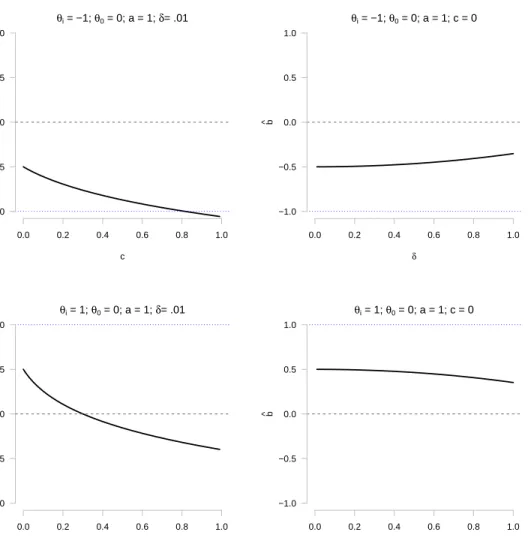
A.2 Maximum of the Expected Log-Likelihood Ratio with respect to θ0 . . . 153
A.3 Maximum of the Expected Log-Likelihood Ratio with respect to b . . . 158
Appendix B. Tables: Aggregate over Distribution 166 B.1 Group Means . . . 167
B.2 Effect Sizes . . . 186
C.1 Scatterplots . . . 197
C.2 Loss Trend Plots . . . 205
Appendix D. Figures: Conditional on Ability 207
D.1 Accuracy Plots . . . 209
D.2 Test Length Plots. . . 221
D.3 Loss Plots . . . 233
List of Tables
6.1 Effect sizes for an ANOVA predicting mean test length given a compen-satory classification bound function. . . 102
6.2 Effect sizes for an ANOVA predicting mean classification accuracy given a compensatory classification bound function. . . 103
6.3 Effect sizes for an ANOVA predicting mean test length given a
non-compensatory classification bound function. . . 105
6.4 Effect sizes for an ANOVA predicting mean classification accuracy given a non-compensatory classification bound function. . . 106
B.1 The average PCC, number of items administered, and loss aggregated within each item selection algorithm assuming a compensatory classifica-tion bound funcclassifica-tion. . . 167
B.2 The average PCC, number of items administered, and loss aggregated within each item selection algorithm assuming a non-compensatory clas-sification bound function. . . 167
B.3 The average PCC, number of items administered, and loss aggregated within each stopping rule assuming a compensatory classification bound function. . . 168
within each stopping rule assuming a non-compensatory classification bound function. . . 168
B.5 The average PCC, number of items administered, and loss aggregated within item bank by ability correlation assuming a compensatory classi-fication bound function. . . 169
B.6 The average PCC, number of items administered, and loss aggregated within item bank by ability correlation assuming a non-compensatory classification bound function. . . 169
B.7 The average PCC, number of items administered, and loss aggregated within ability correlation by item selection algorithm assuming a com-pensatory classification bound function. . . 170
B.8 The average PCC, number of items administered, and loss aggregated within ability correlation by item selection algorithm assuming a non-compensatory classification bound function. . . 171
B.9 The average PCC, number of items administered, and loss aggregated within ability correlation by stopping rule assuming a compensatory clas-sification bound function. . . 172
B.10 The average PCC, number of items administered, and loss aggregated within ability correlation by stopping rule assuming a non-compensatory classification bound function. . . 173
B.11 The average PCC, number of items administered, and loss aggregated within item bank by item selection algorithm assuming a compensatory classification bound function. . . 174
within item bank by item selection algorithm assuming a non-compensatory classification bound function. . . 175
B.13 The average PCC, number of items administered, and loss aggregated within item bank by stopping rule assuming a compensatory classification bound function. . . 176
B.14 The average PCC, number of items administered, and loss aggregated within item bank by stopping rule assuming a non-compensatory classi-fication bound function. . . 177
B.15 The average PCC and number of items administered within item selection algorithm by stopping rule assuming a compensatory classification bound function and a between multidimensional item bank. . . 178
B.16 Various loss values within item selection algorithm by stopping rule as-suming a compensatory classification bound function and a between mul-tidimensional item bank.. . . 179
B.17 The average PCC and number of items administered within item selection algorithm by stopping rule assuming a compensatory classification bound function and a within multidimensional item bank. . . 180
B.18 Various loss values within item selection algorithm by stopping rule as-suming a compensatory classification bound function and a within mul-tidimensional item bank.. . . 181
B.19 The average PCC and number of items administered within item selection algorithm by stopping rule assuming a non-compensatory classification bound function and a between multidimensional item bank. . . 182
suming a non-compensatory classification bound function and a between multidimensional item bank.. . . 183
B.21 The average PCC and number of items administered within item selection algorithm by stopping rule assuming a non-compensatory classification bound function and a within multidimensional item bank. . . 184
B.22 Various loss values within item selection algorithm by stopping rule as-suming a non-compensatory classification bound function and a within multidimensional item bank.. . . 185
B.23 Effect sizes for an ANOVA predicting mean classification accuracy given a compensatory classification bound function. . . 186
B.24 Effect sizes for an ANOVA predicting mean test length given a compen-satory classification bound function. . . 187
B.25 Effect sizes for an ANOVA predicting average loss withP = 100 given a compensatory classification bound function. . . 188
B.26 Effect sizes for an ANOVA predicting average loss withP = 500 given a compensatory classification bound function. . . 189
B.27 Effect sizes for an ANOVA predicting average loss with P = 1000 given a compensatory classification bound function. . . 190
B.28 Effect sizes for an ANOVA predicting mean classification accuracy given a non-compensatory classification bound function. . . 191
B.29 Effect sizes for an ANOVA predicting mean test length given a non-compensatory classification bound function. . . 192
B.30 Effect sizes for an ANOVA predicting average loss withP = 100 given a non-compensatory classification bound function. . . 193
non-compensatory classification bound function. . . 194
B.32 Effect sizes for an ANOVA predicting average loss with P = 1000 given a non-compensatory classification bound function. . . 195
List of Figures
3.1 The expected derivative of the SPRT log-likelihood ratio test statistic for
various values ofθ0. . . 31
3.2 Difficulty parameters that optimize the SPRT log-likelihood ratio. . . . 35
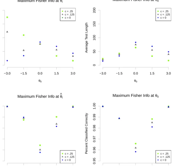
3.3 Average test length and classification accuracy using an SPRT stopping rule with different item selection algorithms, classification bounds, and lower asymptotes.. . . 39
3.4 Average test length using an SPRT stopping rule with different classifi-cation bound-based item selection algorithms, classificlassifi-cation bounds, and lower asymptotes.. . . 43
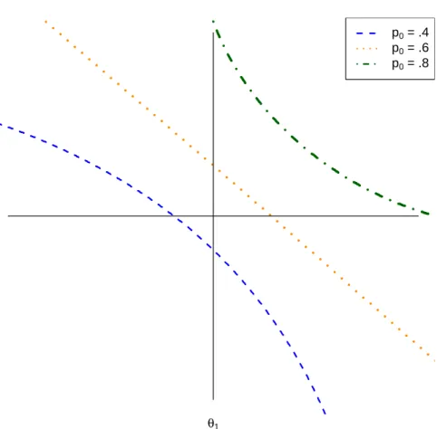
4.1 Classification bound functions assuming a constant, model-predicted prob-ability for passing the test. . . 56
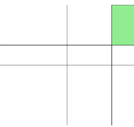
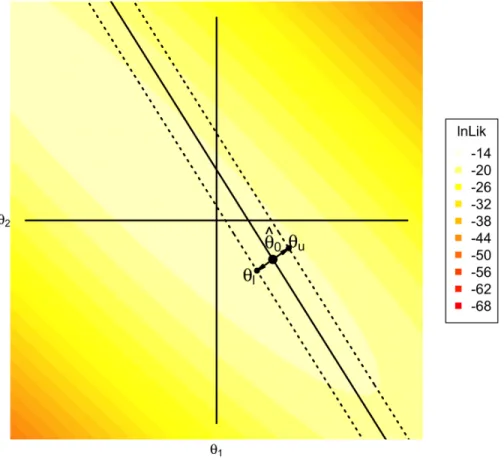
4.2 A diagram of the non-compensatory classification task.. . . 58
4.3 A diagram of the compensatory classification task. . . 59
4.4 A diagram of the Constrained SPRT in two dimensions. . . 64
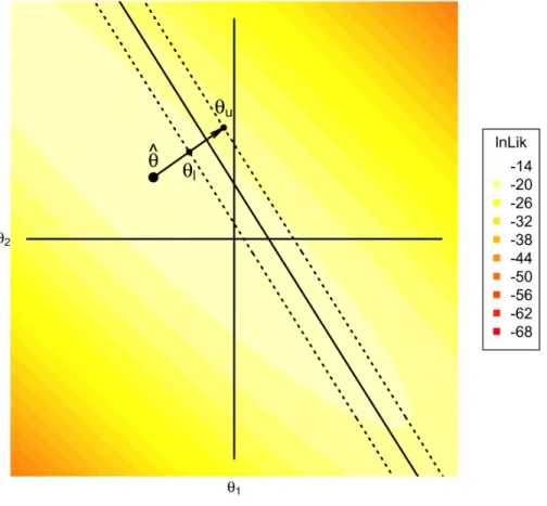
4.5 A diagram of the Projected SPRT in two dimensions. . . 66
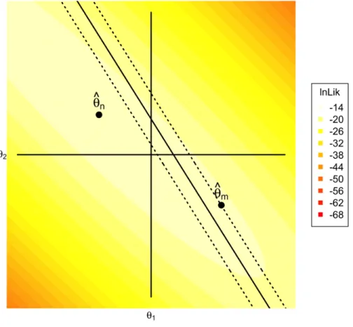
4.6 A diagram of the Multidimensional GLR in two dimensions. . . 68
6.1 Scatterplots of the percent classified correctly by average number of items administered for different item selection algorithms and stopping rules. . 89
6.3 Scatterplots of the percent classified correctly by average number of items administered based on the interaction between item bank and item selec-tion algorithm. . . 95
6.4 Average loss within each item selection algorithm by item bank or stop-ping rule by item bank. . . 97
6.5 Scatterplots of the percent classified correctly by average number of items administered based on the interaction between item bank and stopping rule. . . 99
6.6 Scatterplots of the conditional accuracy rate when using the
compen-satory classification bound function and the C-SPRT stopping rule with δ=.25. . . 108
6.7 Scatterplots of the conditional accuracy rate when using the
compen-satory classification bound function and the M-GLR stopping rule with δ=.25. . . 110
6.8 Scatterplots of the conditional accuracy rate when using the
compen-satory classification bound function and the BCR stopping rule with α=.10. . . 111
6.9 Scatterplots of the conditional average test length when using the com-pensatory classification bound function and the C-SPRT stopping rule withδ=.25. . . 113
6.10 Scatterplots of the conditional average test length when using the com-pensatory classification bound function and the M-GLR stopping rule withδ=.15. . . 114
pensatory classification bound function and the BCR stopping rule with α=.05. . . 115
6.12 Scatterplots of the conditional accuracy rate when using the non-compensatory classification bound function and the C-SPRT stopping rule withδ=.25. 117
6.13 Scatterplots of the conditional accuracy rate when using the non-compensatory classification bound function and the M-GLR stopping rule withδ =.25. 118
6.14 Scatterplots of the conditional accuracy rate when using the non-compensatory classification bound function and the BCR stopping rule withα=.10. . 119
6.15 Scatterplots of the conditional accuracy rate when using the non-compensatory classification bound function and the M-SCSPRT stopping rule with δ=.25. . . 120
6.16 Scatterplots of the conditional average test length when using the non-compensatory classification bound function and the C-SPRT stopping rule withδ=.25. . . 122
6.17 Scatterplots of the conditional average test length when using the non-compensatory classification bound function and the M-GLR stopping rule withδ=.25. . . 123
6.18 Scatterplots of the conditional average test length when using the non-compensatory classification bound function and the BCR stopping rule withα=.10. . . 124
6.19 Scatterplots of the conditional average test length when using the non-compensatory classification bound function and the BCR stopping rule withα=.05. . . 125
C.1 Scatterplots of the percent classified correctly by average number of items administered for different true ability correlations and item banks. . . . 197
administered for different item selection algorithms and stopping rules. . 198
C.3 Scatterplots of the percent classified correctly by average number of items administered based on the interaction between true ability correlation and item bank.. . . 199
C.4 Scatterplots of the percent classified correctly by average number of items administered based on the interaction between true ability correlation and item selection algorithm. . . 200
C.5 Scatterplots of the percent classified correctly by average number of items administered based on the interaction between true ability correlation and stopping rule. . . 201
C.6 Scatterplots of the percent classified correctly by average number of items administered based on the interaction between item bank and item selec-tion algorithm. . . 202
C.7 Scatterplots of the percent classified correctly by average number of items administered based on the interaction between item bank and stopping rule. . . 203
C.8 Scatterplots of the percent classified correctly by average number of items administered based on the interaction between item selection algorithm and stopping rule. . . 204
C.9 Average loss within each item selection algorithm or stopping rule. . . . 205
C.10 Average loss within each item selection algorithm by item bank or stop-ping rule by item bank. . . 206
D.1 Legends for the conditional accuracy, test length, and loss function plots. 208
satory classification bound function and the C-SPRT stopping rule with δ=.25. . . 209
D.3 Scatterplots of the conditional accuracy rate when using the compen-satory classification bound function and the M-SCPRT stopping rule with δ=.25. . . 210
D.4 Scatterplots of the conditional accuracy rate when using the compen-satory classification bound function and the M-GLR stopping rule with δ=.15. . . 211
D.5 Scatterplots of the conditional accuracy rate when using the compen-satory classification bound function and the M-GLR stopping rule with δ=.25. . . 212
D.6 Scatterplots of the conditional accuracy rate when using the compen-satory classification bound function and the BCR stopping rule with α=.05. . . 213
D.7 Scatterplots of the conditional accuracy rate when using the compen-satory classification bound function and the BCR stopping rule with α=.10. . . 214
D.8 Scatterplots of the conditional accuracy rate when using the non-compensatory classification bound function and the C-SPRT stopping rule withδ=.25. 215
D.9 Scatterplots of the conditional accuracy rate when using the non-compensatory classification bound function and the M-SCSPRT stopping rule with δ=.25. . . 216
D.10 Scatterplots of the conditional accuracy rate when using the non-compensatory classification bound function and the M-GLR stopping rule withδ =.15. 217
classification bound function and the M-GLR stopping rule withδ =.25. 218
D.12 Scatterplots of the conditional accuracy rate when using the non-compensatory classification bound function and the BCR stopping rule withα=.05. . 219
D.13 Scatterplots of the conditional accuracy rate when using the non-compensatory classification bound function and the BCR stopping rule withα=.10. . 220
D.14 Scatterplots of the conditional average test length when using the com-pensatory classification bound function and the C-SPRT stopping rule withδ=.25. . . 221
D.15 Scatterplots of the conditional average test length when using the com-pensatory classification bound function and the M-SCSPRT stopping rule withδ=.25. . . 222
D.16 Scatterplots of the conditional average test length when using the com-pensatory classification bound function and the M-GLR stopping rule withδ=.15. . . 223
D.17 Scatterplots of the conditional average test length when using the com-pensatory classification bound function and the M-GLR stopping rule withδ=.25. . . 224
D.18 Scatterplots of the conditional average test length when using the com-pensatory classification bound function and the BCR stopping rule with α=.05. . . 225
D.19 Scatterplots of the conditional average test length when using the com-pensatory classification bound function and the BCR stopping rule with α=.10. . . 226
compensatory classification bound function and the C-SPRT stopping rule withδ=.25. . . 227
D.21 Scatterplots of the conditional average test length when using the non-compensatory classification bound function and the M-SCSPRT stopping rule withδ=.25. . . 228
D.22 Scatterplots of the conditional average test length when using the non-compensatory classification bound function and the M-GLR stopping rule withδ=.15. . . 229
D.23 Scatterplots of the conditional average test length when using the non-compensatory classification bound function and the M-GLR stopping rule withδ=.25. . . 230
D.24 Scatterplots of the conditional average test length when using the non-compensatory classification bound function and the BCR stopping rule withα=.05. . . 231
D.25 Scatterplots of the conditional average test length when using the non-compensatory classification bound function and the BCR stopping rule withα=.10. . . 232
D.26 Scatterplots of the conditional average loss when using the compensatory classification bound function and the C-SPRT stopping rule withδ=.25. 233
D.27 Scatterplots of the conditional average loss when using the compensatory classification bound function and the M-SCSPRT stopping rule withδ= .25. . . 234
D.28 Scatterplots of the conditional average loss when using the compensatory classification bound function and the M-GLR stopping rule withδ =.15. 235
classification bound function and the M-GLR stopping rule withδ =.25. 236
D.30 Scatterplots of the conditional average loss when using the compensatory classification bound function and the BCR stopping rule withα=.05. . 237
D.31 Scatterplots of the conditional average loss when using the compensatory classification bound function and the BCR stopping rule withα=.10. . 238
D.32 Scatterplots of the conditional average loss when using the non-compensatory classification bound function and the C-SPRT stopping rule withδ=.25. 239
D.33 Scatterplots of the conditional average loss when using the non-compensatory classification bound function and the M-SCSPRT stopping rule with δ=.25. . . 240
D.34 Scatterplots of the conditional average loss when using the non-compensatory classification bound function and the M-GLR stopping rule withδ =.15. 241
D.35 Scatterplots of the conditional average loss when using the non-compensatory classification bound function and the M-GLR stopping rule withδ =.25. 242
D.36 Scatterplots of the conditional average loss when using the non-compensatory classification bound function and the BCR stopping rule withα=.05. . 243
D.37 Scatterplots of the conditional average loss when using the non-compensatory classification bound function and the BCR stopping rule withα=.10. . 244
Chapter 1
Introduction
Forty-five states have already adopted the Common Core State Standards (CCSS; 2010) to implement the dictates demanded by No Child Left Behind (NCLB; 2008). As explained on their website, the standards promise to adequately: (1) prepare students for college and work; (2) train students to compete in the global marketplace; and (3) determine student proficiency based on evidence of success (CCSS; 2010). Two state-led groups have been awarded federal funds to design assessments measuring objectives outlined in the CCSS. Due to the quantity of examinees, the high cost of exam develop-ment and impledevelop-mentation, and the consequence of mismeasuredevelop-ment, these assessdevelop-ments should quickly and accurately measure student readiness and achievement. Addressing the concerns of test developers, adaptive testing procedures base item selection and test length on the needs of an assessment and the responses of examinees to already admin-istered items. Due to purported accuracy and efficiency, one of the state-led groups, the Smarter Balanced Assessment Consortium (SBAC; 2013), will soon adopt computerized adaptive tests (CAT; e.g., Wainer, 2000; Weiss, 1982) in high stakes exams (e.g., Way, Twing, Camara, Sweeney, Lazar, & Mazzeo, 2010).
Many tests, such as those constructed by the SBAC, seek to track individual changes
in ability. Another broad set of tests classifies examinees into categories based on the estimated location of ability relative to pre-specified cut-points. The most basic of the latter task-type determines classification by comparing ability to the minimal ability required for demonstrating competence in a particular field (e.g., Kingsbury & Weiss, 1983; Welch & Frick, 1993). For example, medical professionals are expected to know and conform to the dictates of their discipline lest they provide inadequate care and endanger patients’ lives. These threshold-ability tests are generally referred to as “mastery” or “certification” tests (Bejar, 1983). Computerized mastery testing (CMT) is a subset of CAT with the intent of assigning examinees to one of two, mutually exclusive categories: one representing mastery and the other indicating non-mastery. Unlike CATs designed for equiprecise measurement (e.g., Weiss, 1982), the procedures implemented in CMT aim only increase the accuracy of certification.
Psychometric models designed for classification are divided into two, general areas: latent class models and latent trait models. Latent class models, such as diagnostic classification models (DCM; Rupp & Templin, 2008), assume that reality consists of a constellation of discrete cognitive states. One determines classification in DCM by estimating the posterior probability of each examinee having the attributes required for mastery given responses to test items. Latent trait models, such as item response theory (IRT; e.g., Embretson & Reise, 2000), assume that each examinee can be represented as a point in RK, where K is the number of dimensions underlying a series of test items. One determines classification in IRT by comparing the location of each examinee’s ability vector in multidimensional space to some boundary curve separating the categories.
Both IRT and DCM can be used as the psychometric model underlying adaptive tests. All adaptive tests must include algorithms to determine which questions should be administered to each examinee and when enough information has been collected to end each test. During equiprecise CAT, questions are generally selected to provide as
much information as possible at the current ability estimate, and tests are generally stopped once that ability estimate has sufficiently stabilized. Conversely, during mas-tery tests, questions are generally selected to provide information about whether the examinee is on either side of the cut-point, and tests are generally stopped once that mastery decision has stabilized. These procedures will often result in drastically dif-ferent tests. For example, imagine Einstein taking an introductory Physics equiprecise CAT. Because scarcely any questions are very difficult, the test would require many questions to differentiate his ability from other Physics professors. However, if the test were designed as a mastery test, only a few questions would be needed before a clear designation of “mastery” could be made.
Most researchers designing CMT algorithms using IRT models have assumed that only one trait underlies responses to test items (although see Glas & Vos, 2010; Seitz & Frey, 2013; and Spray, Abdel-fatah, Huang & Lau, 1997). Item selection algorithms for unidimensional, IRT-based mastery tests include selecting items by maximizing: (1) Fisher information at the classification bound (e.g., Eggen, 1999; Lin & Spray, 2000; Spray & Reckase, 1994); (2) Kullback-Leibler divergence at the classification bound (e.g., Eggen, 1999); and (3) the weighted log-odds ratio at the classification bound (e.g., Lin, 2011; Lin & Spray, 2000). Stopping rules for unidimensional, IRT-based mastery tests fall into two general categories: (1) Bayesian decision rules (e.g., Lewis & Shehan, 1990; Rudner, 2009); and (2) sequential decision theory (e.g., Bartroff, Finkel-man, & Lai, 2008; Eggen, 1999; FinkelFinkel-man, 2010; Thompson, 2009). The Bayesian decision approach to mastery testing determines, after each step, the posterior expected loss given prior information, classification proportions, and a set of responses. A test is then terminated if the expected loss for making a specific classification/decision is sufficiently small. In contrast, sequential decision theory algorithms are generally based off of Wald’s (1945; 1947) Sequential Probability Ratio Test (SPRT), which uses a
likelihood ratio test statistic to determine when enough independent and identically distributed (i.i.d.) data have been collected to choose between one of two simple hy-potheses. For unidimensional IRT-based CMT algorithms, these simple hypotheses are usually chosen to be specific ability values slightly within each category (e.g., Reck-ase, 1983). Then, after administering an item to an examinee, the SPRT must decide whether that examinee should be classified in the lower category, the examinee should be classified in the upper category, or the examinee should be administered another item. Primary justification for using the SPRT in mastery tests is attributed to the Wald-Wolfowitz theorem: given two simple hypotheses, “of all tests with the same power the sequential probability ratio test requires on the average fewest observations” (Wald & Wolfowitz, 1948). Because conditions underlying SPRT optimality do not generally apply to CMTs (see Nydick, 2012, for criticisms of the SPRT as applied to CMTs), researchers have proposed extensions of/alternatives to the simple SPRT, including the Generalized Likelihood Ratio Test (GLR; Bartroff, Finkelman, & Lai, 2008; Thompson, 2009), the SPRT with Stochastic Curtailment (SCSPRT; Finkelman, 2008a), and the SPRT with Predictive Power (Finkelman, 2010). The latter two methods, based off of probabilistic stopping rules taken from the clinical trials literature (Lan, Simon, & Halperin, 1982), determine whether to terminate an exam based, in part, on information from the remaining items in the bank.
Certification tests often aim to assess a composite of dimensions, but those tests gen-erally provide a total score assumed to capture relevant information about that compos-ite. For example, radiographers must know physics (how to use equipment), medicine (how to find the the appropriate anatomical area in a picture), patient care (how to make patients feel comfortable), etc. All of these dimensions are probably correlated to some degree, yet they are distinct enough to result in separate types of questions. Unfortunately, the criterion used to make a decision about the examinee’s certification
is generally based on the total test score (Interpreting, 2003, p. 23). To classify an examinee along two dimensions using unidimensional IRT, one must make two separate decisions or, worse, pretend that those dimensions are perfectly correlated (although see Seitz & Frey and Spray et al., 1997, for alternative conceptions of “unidimensional al-gorithms” as applied to a multidimensional classification task). Multidimensional item response theory models are more flexible in accounting for relationships between these underlying dimensions unless those dimensions are highly correlated (Ackerman, 1989). The purpose of this thesis is to extend the theory of unidimensional IRT-based computerized mastery testing to multidimensional IRT models and then to compare the proposed algorithms in a large simulation study. The remainder of this thesis is organized as follows. In Chapter 2, I explain the unidimensional three-parameter IRT model and review the most commonly used item selection algorithms and stopping rules in computerized mastery testing. In Chapter 3, I show how the optimal method of se-lecting items for unidimensional CMT depends on the IRT model used and the location of true ability relative to the classification bound. In Chapter 4, I describe the most commonly used multidimensional IRT models and extend unidimensional conceptualiza-tions of mastery (including the item selection algorithms and stopping rules) to multiple dimensions. In Chapter 5, I outline a simulation study designed to compare many of the proposed multidimensional CTM algorithms in realistic testing situations. In Chapter 6, I summarize results from the simulation, and in Chapter 7, I draw conclusions from the simulation and propose future directions.
Chapter 2
Unidimensional Algorithms
In this chapter, I briefly outline the unidimensional, binary IRT model and explain currently used item selection algorithms and stopping rules for unidimensional adaptive mastery testing.
2.1
Unidimensional IRT and Mastery Testing
Item response theory (IRT) is a mathematical model that describes the relation-ship between responses to test items and examinee ability. The most popular IRT model remains the unidimensional, binary, three-parameter logistic model (3PL; Birn-baum, 1968) or simplifications thereof. Specifically, letθrepresent the continuous latent variable underlying examinee responses to test items, assume that responses are con-ditionally independent1 given a fixed θ = θi (where i indexes examinees), and allow responses to have two possible scores, 0 and 1. Then, according to the 3PL, the proba-bility of examineeicorrectly responding to itemj (i.e., getting a score of 1 on the item) is defined by the following item response function (IRF):
1
For adaptive tests, “conditionally independent” is a more appropriate assumption than “locally independent” due to item selection dependencies (e.g., Mislevy & Chang, 2000).
pj(θi) = Pr(Yij = 1|θi, aj, bj, cj) =cj+
1−cj
1 + exp[−Daj(θi−bj)]
, (2.1)
where bj denotes the inflection point of the IRF, aj is proportional to the slope of the IRF at its inflection point,cj indicates the lower asymptote, andDis a scaling constant usually specified to be either 1 (for the logistic metric) or 1.7022 (for the normal-ogive metric), although alternative numbers for D have been proposed3. Because D is a scaling constant that does not affect model fit, I will let D = 1 for clarity. Common restrictions of the 3PL for binary items include: (1) eliminating the lower-asymptote parameter across all items, which results in a two-parameter model (2PL) specified by the following IRF:
pj(θi) = Pr(Yij = 1|θi, aj, bj) =
1
1 + exp[−aj(θi−bj)]
; (2.2)
and (2) restricting the slope parameters across items to be identical, which results in a one-parameter (1PL) model, and can be written with the following IRF:
pj(θi) = Pr(Yij = 1|θi, bj) =
1
1 + exp[−a(θi−bj)]
. (2.3)
Unidimensional models assume that a single ability underlies responses to all items on a test or in an item bank. Therefore, unidimensional mastery can be defined as a range of values on this latent dimension separated by a cut-score, θ0. For examinee i,
the correct mastery decision depends on the location of θi relative to θ0. If θi > θ0,
the examinee should be classified as a master and any other decision is a Type II error. Conversely, if θi< θ0, then the examinee should be classified as a failure and any other
2D= 1.702 minimizes the maximum difference between the normal and logistic cumulative
distribu-tion funcdistribu-tions (Camilli, 1994).
3D = 1.749 minimizes the KL-divergence between the normal and logistic densities assuming the
decision is a Type I error (Finkelman, 2008a). Unidimensional item selection algorithms and stopping rules were derived to result in the shortest tests conditional on pre-specified Type I and Type II error rates. In the next two sections, I briefly outline each of the commonly used item stopping rules and item selection algorithms in unidimensional CMT. Because efficient CMT item selection algorithms depend on the stopping rule, I first describe commonly used stopping rules and then explain how those classification criteria inform item selection decisions.
2.2
Unidimensional Stopping Rules
Many of the stopping rules in computerized mastery testing are modifications of Wald’s Sequential Probability Ratio Test (SPRT; Wald, 1947). Therefore, I briefly outline the SPRT as applied to CMT and then review CMT-based modifications of the SPRT designed to circumvent its shortcomings.
2.2.1 The Sequential Probability Ratio Test
The classic stopping rule in CMT, the SPRT algorithm (e.g., Eggen, 1999; Reckase, 1983; Spray & Reckase, 1996), simplifies the classification task. Assume that a test administrator must classify examinees into one of two categories separated by a cut-point. Let θ0 denote this a priori selected ability value separating true failures from
true masters. Then point hypotheses can be specified as
H0 :θi =θ0−δ
H1 :θi =θ0+δ
inside of the mastery region.
The purpose of any stopping rule in CMT is to determine whether an examinee should be classified as a master, a non-master, or be administered another item. To make one of these three decisions, the SPRT compares the likelihood ratio test statistic to appropriate critical values. As an example of how the likelihood ratio statistic might be applied, let responses be conditionally independent and follow the unidimensional, binary, item response function defined in Equation (2.1). Then the log-likelihood for a single examinee given a particular response pattern, yi, J = [yi1, yi2, . . . , yiJ]T, is
log[L(θ|yi, J)] = J X j=1 h yijlog[pj(θ)] + (1−yij) log[1−pj(θ)] i (2.4)
with pj(θ) defined in Equation (2.1). If H0 :θl =θ0−δ and H1 :θu =θ0+δ, then the
log-likelihood ratio of examineei manifestingθu relative toθl is
Ci, j = log h LR(θu, θl|yi, j) i = log L(θ u|yi, j) L(θl|yi, j) = loghL(θu|yi, j) i −loghL(θl|yi, j) i . (2.5) When Equation (2.5) is a large, positive number, then there is sizable evidence that θu generated the particular response pattern, yi, j. Conversely, when Equation (2.5) is a large, negative number, there is considerable evidence supporting θl.
Justification for using a likelihood ratio test statistic when testing simple hypothe-ses is due to the Neyman-Pearson lemma (Casella & Berger, 2001, p. 366). Accord-ing to the Neyman-Pearson lemma, for a fixed sample size, N, and conditional on a particular Type I error rate, α, the uniformly most powerful (UMP) test rejects H0 only contingent on the size of the likelihood ratio test statistic. Likelihood
Wald-Wolfowitz theorem (Wald & Wolfowitz, 1948). Specifically, let Y1, Y2, . . . be a
(possibly infinite) independent and identically distributed (i.i.d.) sample from com-mon density f with unknown parameter vector θ (dim(θ) ≥ 1). Then assuming a pair of simple hypotheses, H0 : θ = θ1 versus H1 : θ = θ2, and pre-specified
crit-ical values, A and B, where 0 < A < B < ∞, a rule that stops sampling when
N = inf n n≥1 : Qni=1 hf(yi|θ 1) f(yi|θ2) i ≤A or Qni=1 hf(yi|θ 1) f(yi|θ2) i ≥B o
is optimal (i.e., min-imizes the expected sample size under both H0 and H1) in the set of all tests with the
same Type I and Type II error rates (Lai, 1997). Using the log-likelihood test statistic (rather than the likelihood) and given specific α (Type I error rate) and β (Type II error rate) levels, Wald (1947) recommended choosing Cl = log[A] = log
h β
1−α i
as the critical value separating non-mastery from uncertainty and Cu = log[B] = log
h
1−β α
i as the critical value separating mastery from uncertainty.
Modeled on sequential decision theory, psychometricians have designed a simple template for ending unidimensional mastery tests. After each item between the min-imum number of items, jmin, and the maximum number of items, jmax, calculate
Ci, j = log
LR(θu, θl|yi, j)
as defined in Equation (2.5). If Ci, j < Cl, classify the examinee as a failure and terminate the test. If Ci, j > Cu, classify the examinee as a master and terminate the test. But if Cl ≤Ci, j ≤Cu, administer another item. Once
j =jmax, use a final critical value of (Cl+Cu)/2 (Finkelman, 2008a) to make a decision. Often, researchers setα=β, so that (Cl+Cu)/2 = 0, but practitioners sometimes desire to avoid one type of error depending on the ultimate costs of misclassification.
Unfortunately, researchers have identified several limitations of the standard SPRT in adaptive mastery testing. First, although Wald and Wolfowitz (1948) proved opti-mality of the SPRT when testing simple hypotheses, the SPRT is inefficient relative to other procedures if θi 6= θl and θi 6= θu (Finkelman, 2008a). In light of this concern, the Generalized Likelihood Ratio (GLR; Bartroff, Finkelman, & Lai, 2008; Thompson,
2009, 2010) was proposed as a simple modification of the SPRT that tests composite hypotheses. Second, the SPRT controls the error rate for infinitely long experiments under certain conditions, but every CAT must be terminated after a maximum number of items. Finkelman (2003, 2008a) proposed several procedures that use the likelihood ratio test statistic to estimate the probability of examinee i switching categories by
jmax. In the next several sub-sections, I explore each of the common adjustments to the
SPRT algorithm.
2.2.2 The Generalized Likelihood Ratio
The Generalized Likelihood Ratio (GLR) is a modification of the simple SPRT algorithm for testing composite hypotheses. To derive the GLR procedure, consider a general version of the simple hypotheses specified above,
H0 :θi≤θl =θ0−δ
H1 :θi≥θu =θ0+δ,
where θ ∈ R has an associated likelihood function f(y|θ). Then using a generalized likelihood ratio test statistic withL(θ1|y) = arg maxθ>θ0{f(y|θ)} in the numerator and
L(θ2|y) = arg maxθ≤θ0{f(y|θ)} in the denominator often results in a uniformly most
powerful (UMP) test (Casella & Berger, 1990, p. 368). Intuitively, the generalized like-lihood approach compares ˆθMLE = arg maxθ∈RL(θ|y) (where MLE stands for Maximum Likelihood Estimate) to the most likely value of the composite hypothesis to which ˆθMLE
does not belong.
Adopting generalized likelihood ratio statistics in sequential analyses, Lai (2001) wrote that “simulation studies and asymptotic analyses have shown that [the number
of items needed to make a decision using a GLR] is nearly optimal over a broad range of parameter values θ, performing almost as well as [a procedure] that assumes θ to be known” (p. 307). Due to its desirable characteristics, Bartroff, Finkelman, and Lai (2008) proposed adopting Gi, j = log h GLR(θ0|yi, j) i = log h L(ˆθ|yi, j) i −log h L(θ0|yi, j) i (2.6)
as an alternative to the simple likelihood ratio in CMT, where θ0 =θ0+δ if ˆθ ≤θ0 or
θ0=θjmax
− if ˆθ > θ0, and θj−max is found via Monte Carlo simulation to yield appropriate
α and β rates. The same procedure is used in GLR as in SPRT with slightly different hypotheses, test statistics, and critical values (which are also found via simulation). Contrary to Bartroff et al. (2008), who proposed complicated methods for determining the test statistic and critical values, Thompson (2009, 2010) suggested that the GLR be identical to “the fixed point SPRT, with the exception thatθ1 andθ2[in the generalized
likelihood ratio test statistic] are allowed to vary” (Thompson, 2010, p. 5). Therefore, Thompson advised calculating
log h GLR(θu, θl|yi, j) i = sup θ1≥θu log h L(θ1|yi, j) i − sup θ2≤θl log h L(θ2|yi, j) i , (2.7)
and comparing the result to Cl and Cu as in the SPRT. Note that Equation (2.7) contrasts the MLE with the maximum of the likelihood in the hypothesis to which the MLE does not belong. Regardless of method, both GLR and SPRT compare some version of a likelihood ratio test statistic to critical values that are only based on the items already taken. Finkelman (2003, 2008a) proposed a supplementary stopping rule, based on the work of Lan, Simon, and Halpern (1982) from the clinical trials literature, that also considers the remaining set of items before making a decision. I next address
the various curtailed decision rules.
2.2.3 The SPRT with Stochastic Curtailment
A curtailed version of a sequential procedure (Eisenberg & Ghosh, 1980) makes decision Di, j =r for examinee i, withj < jmax, if and only if for everys6=r, decision
Di, jmax = s can not happen. In other words, the curtailment criterion results in a
decision if and only if all other decisions are impossible by the maximum sample size. Because a curtailment criterion is usually difficult to obtain, researchers have modified curtailed stopping rules to make decision Di, j =r for examineei, withj < jmax, if and
only if for everys6=r, the probability of deciding Di, jmax =sis below some probability
threshold (Finkelman, 2008a, p. 453). As applied to mastery testing, the SPRT with Stochastic Curtailment (SCSPRT; Finkelman, 2003) classifies an examinee when the probability of the examinee being classified in the other category byjmax is small.
To derive the stochastically curtailed SPRT, let Di, jtmp be the temporary decision
after jtmp < jmax items, and assume that an SPRT-based mastery decision has not
been made by jtmpitems. SetDjtmp =n(wherenstands for “non-master”) ifCi, jtmp <
(Cl+Cu)/2, and setDi, jtmp =dm(wheremstands for “master”) ifCi, jtmp >(Cl+Cu)/2.
Next, pick two error rates, 0 ≤1 ≤.5 and 0 ≤2 ≤.5. Finally, classify the examinee
as a non-master if {Ci, jtmp < Cl} or{Djtmp =nand Pr(Di, jmax =n|Ci, jtmp)≥1−1};
alternatively, classify the examinee as a master if {Ci, jtmp > Cu} or {Djtmp = m and
Pr(Di, jmax = m|Ci, jtmp) ≥ 1−2}. Notice how Finkelman (2008a) defined four error
rates. α and β are the specified Type I and Type II error rates for an examinee at a particular end of the indifference region given an infinitely long experiment. Conversely,
1 and2 are the specified Type I and Type II error rates for an examinee classified in a
particular category at the hypothetical end of the test. Unlike α and β,1 and 2 refer
To determine the SCSPRT decision rule, one must derive the probability of switching categories by maximum test length. Finkelman (2008a) used a normal approximation to the log-likelihood function after jmaxitems conditional onjtmp< jmax items already
administered. Specifically, define C0= (Cl+Cu)/2. Then afterjtmp< jmax items,
Prθ˜(Di, jmax =n|Ci, jtmp) = 1−Prθ˜(Di, jmax =m|Ci, jtmp)≈Φ C0−Eθ˜(Ci, jmax|Ci, jtmp) p Varθ˜(Ci, jmax|Ci, jtmp) ! (2.8) where Eθ˜(Ci, jmax|Ci, jtmp) =Ci, jtmp+ jmax X j=jtmp+1 Eθ˜ log L(θu|Yij) L(θl|Yij) , (2.9) Varθ˜(Ci, jmax|Ci, jtmp) = jmax X j=jtmp+1 Varθ˜ log L(θu|Yij) L(θl|Yij) , (2.10) ˜
θis the assumed ability under which the expectation/variance are evaluated, and Φ(·) is the CDF of a standard normal distribution. One can straightforwardly calculate these probabilities as long as the remaining jtmp+ 1 to jmax are known in advance (or can
be guessed) and if jtmp+ 1 << jmax for the Central Limit Theorem to apply (e.g.,
Finkelman, 2008a, p. 450). Non-nested likelihood ratio test statistics generally use an asymptotic normal distribution rather than a χ2 distribution (Vuong, 1989).
Finkelman (2008a) proved that under mild sequential conditions, the SCSPRT re-placing a generalized version4 of the SPRT is weakly admissible5. Intuitively, Finkelman
4
A generalized version of the SPRT is identical to the fixed-point SPRT with (potentially) step-dependent critical values. See Eisenberg, Gosh, and Simons (1976; as cited in Finkelman, 2008).
5
A decision method is weakly admissible if no alternative method exists with at most as large error rates (with one of those error rates strictly smaller) and an almost-surely smaller number of sequential steps. See Eisenberg and Simons (1978; as cited in Finkelman, 2008).
(2008a) explained that weak admissibility of the SCSPRT results from stochastic cur-tailment “[eliminating] the use of all ‘wasted’ items, that is, all items that cannot affect the classification decision” (p. 455). Unfortunately, the Expectation and Variance in the Equations (4.15)–(4.16) are taken with respect to a particular θ: the closest end-point of the indifference region, the current ability estimate, or (as Finkelman, 2008a, 2010, recommended) the endpoint of a confidence interval closest to the classification bound. Finkelman (2010) proposed a less ad hoc approach by weighting the conditional probability estimate on the distribution ofθi afterjtmp items.
2.2.4 The SPRT with Predictive Power
Finkelman (2010) proposed several modifications of the stocastically curtailed SPRT stopping rule for computerized adaptive mastery tests. One option (termed “MLE formation”) takes the expectation and variance of the likelihood ratio test statistic with respect to ˜θ = ˆθMLE rather than ˜θ = θl or ˜θ = θu once estimates of ˆθMLE stabilize.
A second option (termed “confidence interval formation”) is identical to the “MLE formation” but uses a confidence interval endpoint in the likelihood ratio test statistic rather than the MLE itself. The final recommendation of Finkelman (2010) (termed “predictive power”) weights the SCSPRT by the posterior distribution of θi after jtmp
items. Specifically, letπ(θ) be the prior distribution ofθ. Then the posterior distribution of θi after jtmpitems can be written
π(θ|yi, jtmp) = R π(θ)L(θ|yi, jtmp)
Θπ(θ)L(θ|yi, jtmp)dθ
, (2.11)
where Θ is the set of allθ,yi, jtmp is the response pattern of examineeiafterjtmpitems,
L(θ|yi, jtmp) is the likelihood function given response pattern yi, jtmp, and, by definition, the integral of a function f(θ), RΘf(θ)dθ, is taken over allθ ∈Θ. Then the PPSPRT
can be defined as
PrΘ(Di, jmax =n|Ci, jtmp) =
Z
Θ
π(θ|yi, jtmp)Prθ(Di, jmax =n|Ci, jtmp)dθ, (2.12)
where PrΘ(Di, jmax = n|Ci, jtmp) is the expected SCSPRT criterion over Θ. If defining
the loss in making a classification decision as
Loss = 100×IW +J, (2.13)
where IW is an indicator function for incorrect classification and J is the number of items given to an examinee, then the PPSPRT and ˜θ = ˆθMLE methods resulted in
the lowest average loss across all conditions (Finkelman, 2010). Therefore, using a PPSPRT stopping rule for mastery tests appears to result in a reasonable tradeoff between average test length and classification accuracy. Although SPRT-based stopping rules are increasingly used in CMT research, an alternative branch of CMT stopping rules are based on Bayesian decision theory.
2.2.5 Bayesian Decision Rules
An alternative set of stopping rules in CMT is based on Bayesian decision theory (e.g., Lewis & Shehan, 1990; Vos, 1999, 2002). Rather than adopting the likelihood ratio test statistic, Bayesian decision rules combine information from the posterior distribu-tion of θi with specified costs in making decisions and administering items. Specifically, let Θm represent the set of masters, such that Θn = Θcm symbolizes the set of non-masters. Assuming that θis a continuous random variable, then
π(m|yi, jtmp) = 1−π(n|yi, jtmp) = Z
Θm
π(θ|yi, jtmp)dθ (2.14) is the posterior probability of mastery given the first jtmp items. Given the posterior
probability of mastery, one can then make a decision after determining: (1) states of nature, (2) possible actions, (3) loss functions, and (4) decision rules/principles. As an example of Bayesian decision theory, Lewis and Sheehan (1990) proposed a simple procedure. Define a mastery test with boundary point,θ0, and possible states of nature,
Θ = {Θn,Θm}. Then, after item j is administered to examinee i, one can either fail the examinee (ˆθi ∈ Θn, where ˆθi is the MLE of θi), pass the examinee (ˆθi ∈ Θm), or administer another item. Each decision incurs a pre-specified cost. Let η1be the cost of
passing an examinee who should not pass the test,η2 be the cost of failing an examinee
who should pass the test, and κ be the cost of administering an additional item. Using Equation (2.14), the expected loss of passing the examinee after item j can be written as
Eθ[L(θ, m)|yi, j] =jκ+η1· 1−π(m|yi, j)
, (2.15)
and the expected loss of failing the examinee after itemj can be written as
Eθ[L(θ, n)|yi, j] =jκ+η2·π(m|yi, j). (2.16)
The expected loss of administering another item depends on its usefulness for ultimately making a decision, and as such, relies on the expected future loss of eventually failing or passing the examinee. Lewis and Sheehan (1990) defined the risk at stage j as the expected loss incurred by making the best decision at that stage. Assuming that the decision afterjmaxitems must be a classification, then the risk at the final stage can be
written
Rjmax(θ|yi, jmax) = min
jmaxκ+η1·(1−π m|yi, jmax) , jmaxκ+η2·π(m|yi, jmax) . (2.17)
Equation (2.17) can then be iteratively used to find the expected loss for administering another item at any jtmp before jmax. Specifically, the expected loss for continuing to
test at stage jtmp can be expressed as a function of the risk at stagejtmp+1,
Eθ[L(θ, c)|yi, jtmp] =pjtmp+1(θ)·Rjtmp+1(θ|[yi, jtmp,1]) + 1−pjtmp+1(θ)
·Rjtmp+1(θ|[yi, jtmp,0]),
(2.18)
where pjtmp+1(θ) is the probability of correctly responding to item jtmp+ 1, as defined
in Equation (2.1), so the risk at stagejtmp< jmax becomes
Rjtmp(θ|yi, jtmp) = min Eθ[L(θ, m)|yi, jtmp], Eθ[L(θ, n)|yi, jtmp], Eθ[L(θ, c)|yi, jtmp] . (2.19) Therefore, the potential risk at stage jtmp depends on the possible risk at stagesjtmp+
1, . . . , jmax. Equation (2.19) terminates in Equation (2.17) because the final stage must
result in a pass/fail decision. After each item, the algorithm would choose the path (pass, fail, continue) that minimizes the corresponding expected loss. Note thatpjtmp+1(θ) and
π m|yi, jtmp+1) must also be iteratively defined based on the distribution of responses given the jtmpth posterior distribution of θ. Lewis and Shehan (1990) found that using a Bayesian decision procedure in lieu of administering a fixed number of items reduced CMTs by approximately 50% with little loss in classification accuracy.
away from the classification bound (e.g., Vos, 1999), and another common decision rule is to minimize the maximum (rather than expected) loss (e.g., Vos, 2002). Regardless of loss function or decision rule, many stopping rules depend on a hypothetical complete test. For unidimensional mastery testing, several possible algorithms are available to choose those future items.
2.3
Unidimensional Item Selection Algorithms
All adaptive testing algorithms require methods of selecting future items. The cur-rent section details common item selection algorithms in adaptive tests and then explains modifications of those algorithms for use in mastery testing.
2.3.1 Fisher Information Methods
Many item selection algorithms require determining the information gained by, and thus the benefit of, choosing one potential future item over another potential future item. Fisher information (FI; Lord, 1980) measures the curvature of the log-likelihood in a small area surrounding the maximum likelihood estimate and relates to the asymptotic variance of ˆθ given true θ (e.g., Frank, 2009). Fisher information for item j can be written as a function of true θ,
Ij(θ) =−E ∂2log[L(θ|y)] ∂θ2 = [p 0 j(θ)] 2 pj(θ)[1−pj(θ)] = a 2 j(1−cj) cj+ exp[aj(θ−bj)] cj+ exp[−aj(θ−bj)] 2 (2.20)
p0j(θ) = dpj(θ)
dθ =
(1−cj)ajexp[aj(θ−bj)] (1 + exp[aj(θ−bj)])2
(2.21)
is the derivative ofpj(θ) with respect toθ. The most common Fisher information-based item selection algorithm administers items that maximize (2.20) atθ= ˆθi. Basic criticisms of the original method include: (1) the likelihood function occassionally does not have a finite maximum (Veerkamp & Berger, 1997), and (2) the MLE estimate is often highly variable toward the beginning of a CAT (Chang & Ying, 1996). Other crit-icisms pertain to classification testing. For instance, if anycj >0, then selecting items based on maximizing Fisher information at ˆθi is not optimal in determining whether
θi ∈Θm (e.g., Chapter 3; Spray & Reckase, 1994; Wiberg, 2003).
A variant of the typical Fisher information-based item selection algorithm is to take a weighted average of the information function across Θ (e.g., Veerkamp & Berger, 1997),
Ij(θ|wij) = Z
Θ
wijIj(θ)dθ, (2.22)
where wij is the weight function for examinee iused for item j. Some common weight functions include wij = 1 iffθ= ˆθi,wij =L(θ|yi, j−1), or wij =π(θ|yi, j−1) (as defined
in Equation 2.11). Using wij = 1 iff θ = ˆθi is equivalent to standard Fisher infor-mation, and the latter two weight functions account for uncertainty in the maximum likelihood estimate. Veerkamp and Berger (1997) found that selecting items by max-imizing likelihood-weighted Fisher information results in slightly shorter average test lengths than selecting items by maximizing Fisher information at ˆθMLE. Another
com-mon algorithm described by Veerkamp and Berger (1997) is to maximize the average Fisher information across an interval. Let ˆθLi be the lower limit of the interval and ˆθRi
an item that maximizes the average information across that interval. Averaging infor-mation across an interval considers many potential ability estimates and, thus, results in a more robust algorithm (as shown on p. 213 of Veerkamp & Berger for extreme values of θ). One could also circumvent the limited knowledge of locally-defined ˆθMLE
by deriving a more globally-defined objective function.
2.3.2 Kullback-Leibler Methods
Chang and Ying (1996) suggested basing item selection on Kullback-Leibler (KL) divergence rather than FI as the information metric. KL divergence (e.g., Kullback, 1959; Kullback & Leibler, 1951) relates to the expected loss when choosing an approx-imate model rather than the correct model. Let f be the true probability distribution of univariate random variable X, and let g be an alternative/approximate distribution of X. Then the KL divergence betweenf and g is defined to be
KL(f||g) =Ef log f(X) g(X) = Z ∞ −∞ f(x) log f(x) g(x) dx, (2.23)
where||stands for “distance” between distributions, KL(f||g)≥0, and the expectation is taken with respect to the true distribution, f. To derive a KL-based index for com-puterized adaptive tests, let θi be the true ability of examinee i. Then KL divergence for the jth item can be defined
KLj(θi||θ) =Eθilog L(θi|Yij) L(θ|Yij) =pj(θi) log pj(θi) pj(θ) + [1−pj(θi)] log 1−pj(θi) 1−pj(θ) . (2.24) As shown by Chang and Ying (1996), the curvature of the KL divergence function at a point is equal to Fisher information at that point. Therefore, KL divergence effectively
reduces to Fisher information if choosing θ to be close to θi. Chang and Ying (1996) recommended using KL divergence because “there is no requirement thatθi be close to
θ” (p. 218), unlike the more local character of Fisher information. Moreover, by using a likelihood ratio statistic, KL divergence is similar to the decision-making process of the SPRT. Several different KL divergence indices have been proposed for use in adaptive testing. Originally, the KL information index was defined as average KL divergence along a small interval,
KLj(ˆθi) =
Z θiˆ+δij
ˆ
θi−δij
KL(ˆθi||θ)dθ, (2.25)
where ˆθi is the MLE of θi before administering item j, and δij is a function of the precision in the MLE. Chen, Ankenmann, and Chang (2000) also noted that, as in Fisher information, weight functions can be applied to KL divergence indices, resulting in KLj(ˆθi|wij) = Z θiˆ+δij ˆ θi−δij wijKL(ˆθi||θ)dθ. (2.26)
They further compared bias, MSE, and item overlap for various FI and KL criteria across CATs designed to estimate θi for each person. Only for extreme ability levels did KL information or weighted Fisher information improve over standard Fisher information in terms of bias, MSE, and item overlap early in a test. Moreover, as they wrote, “differences among all [item selection algorithms] with respect to BIAS, RMSE, SE, and item overlap were negligible for tests of more than 10 items” (p. 253, and see Cheng and Lio, 2000, for a partial replication of this study with nearly identical results).
All of the item selection algorithms heretofore discussed were derived to pinpoint an examinee’s true ability. None of the algorithms as presented can be used to efficiently decide whether an examinee is in one of two broadly defined categories. In Chapter 3, I
show why each of the aforementioned algorithms results in inefficient CMTs. However, before explaining reasons for inefficiencies, I first describe alternatives to the typical item selection algorithms appropriate for unidimensional adaptive mastery tests.
2.3.3 Mastery Testing Methods
Many researchers have suggested modifications of the above algorithms for use in mastery testing. For instance, Eggen (1999) promoted selecting items by maximiz-ing Fisher information at θ0 rather than ˆθi or maximizing point-wise KL divergence (Equation 2.24) at KLj(θu||θl). He found that maximizing Fisher information at the cut-point resulted in the shortest and most accurate tests, but selecting items to maxi-mize Fisher information at ˆθi or KL divergence using KLj(θu||θl) did not result in much performance decrement (although see Eggen, 2010 for a replication of Eggen, 1999 with slightly different results).
A common complaint in using point-wise KL divergence in mastery testing is the lack of symmetry between KLj(θu||θl) and KLj(θl||θu). Recall that KL divergence is defined as the expected log-likelihood ratio comparing the true model to an alternative model with respect to the true model. Therefore, when choosing items by maximizing KLj(θu||θl), one implicitly assumes that every examinee is a master. Alternative mastery testing item selection algorithms have been developed that better consider the actual location of an examinee when selecting items. These alternative algorithms include the weighted log-odds ratio (LO; Lin & Spray, 2000) and mutual information (MI; Weissman, 2007). The weighted log-odds ratio selects items that maximize the expected log-odds at the ends of the indifference region,
LOj(θu||θl) = X y Elog pj(θu) pj(θl) Y ÷ 1−pj(θu) 1−pj(θl) 1−Y! (2.27) =E(Y = 1) log pj(θu) pj(θl) −[1−E(Y = 1)] log 1−pj(θu) 1−pj(θl) , (2.28)
whereE(Y = 1) is the classical difficulty of an item and can be calculated by integrating the probability of response for θ weighted on the density of θ across the examinee distribution6.
Mutual information generalizes log-likelihood-based information criteria across mul-tiple cut-points. Weissman (2007) proposed MI as a symmetric version of KL diver-gence. Let ΘB be a discrete set describing the classification bound(s). In our case, ΘB ={θl, θu}. Then mutual information can be defined as
MIj(ΘB) = X y X θ∈ΘB f(y, θ) log f(y, θ) f(y)f(θ) =X y X θ∈ΘB Prj(Y =y|θ)π(θ) log Prj(Y =y|θ) f(y) , (2.29)
where Prj(Y =y|θ) is the probability of Y =y given a particular θ, π(θ) is the prior probability of θ, and f(y) is the marginal probability of Y = y. Lin (2011) tested FI, KL, LO, and MI in several SPRT-based CMTs. He found that the weighted log-odds ratio resulted in the fewest number of items administered, and mutual information resulted in the most number of items administered. All of the algorithms had similar classification accuracies. In Chapter 4, I discuss generalizations of the item selection
6
Lin and Spray, 2000 and Lin, 2011 take the expectation in Equation (2.27) with respect to the marginal distribution ofθ to arrive at Equation (2.28). However, I found taking the expectation with respect to a single examinee’s ˆθi to better reflect the associated SPRT stopping rule. The latter item
and stopping rules to multidimensional adaptive tests. But first, I explain limitations of using certain item selection rules in adaptive mastery tests as a partial justification for deriving particular multidimensional mastery testing item selection algorithms.
Chapter 3
SPRT and Binary Response
Models
A potential limitation of using the SPRT as a decision rule in unidimensional clas-sification tests is due to the non-zero lower asymptote of the three-parameter logistic model. Spray and Reckase (1994) noticed that when using the 3PL, “selecting items to have maximum information at the examinee’s true ability results in longer average test lengths” (p. 9) than selecting items to have maximum information at the cut-points, and “this result is quite dramatic for the lower [classification bound] and examinees above
θ of .5” (p. 9). In other words, the SPRT is inefficient for high ability simulees when using the three-parameter logistic model and selecting items based on the maximum likelihood estimate. Spray and Reckase (1994) proposed a simple method of reducing the number of administered items in SPRT-based classification tests: select items to maximize information at the cut-point separating categories. However, the ideal item selection point depends on the true item and person parameters as well as the classi-fication bound. Selecting items to maximize information at the classiclassi-fication bound is
only a coarse approximation of the most efficient item selection algorithm. By exam-ining properties of IRT log-likelihood ratios, one can shed light on optimal methods of designing item banks, choosing item selection algorithms, and selecting classification criteria for adaptive tests. Because multidimensional IRT models are generalizations of the unidimensional functional form, many of these results should also apply to multi-dimensional adaptive tests. In the following sections, I present the effect of item and person parameters on the magnitude of the SPRT test statistic in two parts: first with mathematical evidence, and then, supporting mathematical conclusions with a small set of simulations.
3.1
Mathematical Considerations
In this section, I demonstrate how the SPRT-based test statistic changes as prop-erties of the logistic model are altered. Thompson (2010), who used the 3PL in his simulations, wrote that “it is far easier to make a classification if the cut-score is in the extremes” and that “typically, only a few items might be needed to classify an examinee above a cut-score of−2.0 or below +2.0” (p. 9). Thompson’s assertion is accurate when using the GLR as a stopping rule (which was the purpose of his paper) but not always when adopting the SPRT. Because his discussion includes research on both stopping rules, his statement of classification efficiency is not entirely correct. Only Spray and Reckase (1994) explicitly acknowledged that “the large difference in number of items for the high ability examinees [when selecting items at proximate estimates of θ rather than at the cut-point] is a result of the nonzero lower asymptote for the three parame-ter logistic model” (p. 7). I now briefly show why non-zero lower asymptotes affect the magnitude of a likelihood ratio test statistic in certain situations. The first part of this section focuses on properties of the classification bound. I then reverse the investigation