Welfare Cost of Business Cycles with Idiosyncratic Consumption Risk and a Preference for Robustness

(1)

Welfare Cost of Business Cycles with Idiosyncratic

Consumption Risk and a Preference for Robustness

∗

Martin Ellison

University of Oxford

Thomas J. Sargent

New York University

September 9, 2014

Abstract

The welfare cost of random consumption fluctuations is known from De Santis (2007) to be increasing in the level of uninsured idiosyncratic consumption risk. It is also known from Barillas et al. (2009) to increase if agents in the economy care about robustness to model misspecification. In this paper, we combine these two effects and calculate the cost of business cycles in an economy with consumers who face idiosyncratic consumption risk and who fear model misspecification. We find that idiosyncratic risk has a greater impact on the cost of business cycles if agents already fear model misspecification. Cor-respondingly, we find that endowing agents with fears about misspecification is more costly when there is already idiosyncratic risk. The combined effect exceeds the sum of the individual effects.

JEL classiﬁcation: E32, E63, D81

Keywords: Cost of Business Cycles, Idiosyncratic Risk, Model Uncertainty, Robustness

∗_{We thank Evan Anderson for helpful comments and Pascal Paul for excellent research assistance. Funding} from the Bank of Korea, the British Academy, and the Oxford Fidelity Research Fund is also gratefully acknowledged.

(2)

1 Introduction

Lucas (1987, 2003) used a calibrated representative agent model to calculate that removing aggregate consumption fluctuations of the size observed in post World War II US data leads to welfare gains equivalent to only 0.1% of the level of consumption each period. Subsequently, researchers have considered variations on the Lucas calculation and identified two modifications that can lead to larger welfare costs of business cycles: changes in the stochastic structure of consumption and changes in the preferences that agents use to value stochastic consumption streams.

The stochastic nature of consumption was changed by De Santis (2007), who calculated the welfare costs of business cycles when individual consumption is subject to both aggregate and idiosyncratic shocks. He found there are large gains to reducing the aggregate component of consumption fluctuations. For example, removing only 10% of the variation induced by aggregate shocks can generate a welfare gain equivalent to 0.5% of the level of consumption each period. Idiosyncratic shocks increase the welfare costs of business cycles because they affect the individual marginal utilities of consumption at which aggregate fluctuations are costed.

How individuals value stochastic streams was the subject of Barillas et al. (2009), who extend the Lucas calculation by assuming that the representative agent has a preference for robustness.1 _{They showed that with a preference for robustness to misspeciﬁcation of the}

consumption process, the welfare gain of removing aggregate fluctuations in consumption can easily exceed 0.5%. Building on the work on ambiguity-averse preferences in Hansen and Sargent (2001), the reasoning is that agents with a preference for robustness are willing to sacrifice a lot to live in an economy without fear of misspecification. The increase in the welfare cost of business cycles arises because concerns about model misspecification cause the representative agent’s worst-case model to put more probability weight on bad consumption shocks.

Our paper combines the insights of De Santis (2007) and Barillas et al. (2009) and argues that the welfare costs of business cycles are important at lower levels of risk aversion and

1_{Tallarini (2000) aimilarly argued that Lucas used the wrong preferences to measure the welfare costs of}

business cycles. Tallarini found that business cycles are costly in a representative agent framework when agents have Epstein-Zin preferences that break the link between risk aversion and the intertemporal elasticity of substitution. Under Tallarini’s interpretation of his model, costly business cycles still require agents to have implausibly high levels of risk aversion when the model is calibrated also to generate an empirically reasonable equity premium and risk free rate.

(3)

fear of model misspeciﬁcation than previously thought. To make the case, we take a model in which agents are subject to aggregate and idiosyncratic consumption shocks and ask what happens if agents fear model misspeciﬁcation. Our framework nests the models of De Santis and Barillas et al. as special cases. To analyze the model we apply the higher order small noise expansion methods for robust economies developed by Anderson et al. (2012).

Recognising that idiosyncratic risk and a fear of model misspecification are in isolation only weak mechanisms for generating welfare costs in economies with low levels of risk aver-sion and very mild fears of model misspecification, it might be expected that introducing the two mechanisms together would not push up the costs of business cycles very much relative to those identified by Lucas. This is not the case; our results go further because the welfare costs of business cycles in our model embody interaction effects between the two mechanisms. The reason is that an agent’s fear of model misspecification extends to its understanding of aggregateand idiosyncratic consumption risks. Agents with a preference for robustness assign additional probability weight both to negative aggregate and to negative idiosyncratic con-sumption shocks, and make decisions to guard against worst-case scenarios in which negative aggregate and idiosyncratic shocks occur simultaneously.

The assumption that agents fear model misspecification addresses a criticism of De Santis (2007), namely, that his analysis relies on highly non-logarithmic preferences to generate an impact of idiosyncratic risk on the costs of aggregate fluctuations. In his baseline calibration the coefficient of relative risk aversion is 2, and most of his headline results are drawn from calculations in which the coefficient of relative risk aversion is set at 4. If the utility function is instead logarithmic in consumption, then the marginal utility of aggregate consumption is completely independent of the level of idiosyncratic consumption, and the welfare costs of business cycles in his model are unaffected by the amount of idiosyncratic risk in the economy. Only if risk aversion is significantly in excess of that implied by logarithmic utility will the costs of business cycles in De Santis differ from those calculated by Lucas. This is no longer the case when agents fear model misspecification. In our model, idiosyncratic risk affects the welfare gains of removing aggregate business cycles even under logarithmic preferences.

The introduction of idiosyncratic risk alternatively speaks to concerns over how to interpret the claim of Barillas et al. (2009) that they only endow agents with mild fears of model misspeciﬁcation. Their calculations for the welfare costs of business cycles assume that agents entertain a relatively large set of models as measured by detection error probabilities based on 235 quarterly observations. Introducing idiosyncratic risk, though, implies that business

(4)

cycles are costly even when the set of models being considered is small. The fears of model misspeciﬁcation needed to make aggregate ﬂuctuations costly are therefore even milder when there is idiosyncratic consumption risk in the economy.

A second issue with De Santis (2007) is that the process he assumes for consumption is problematic empirically. Whilst he goes to some trouble to justify his random walk processes in aggregate and idiosyncratic consumption by appealing to a no-trade theorem, the idea that all variation in consumption growth can be attributed to a random walk process for individual consumption does not fit with empirical studies. For example, Blundell at al. (2008) explicitly focus on the extent of consumption smoothing that different individuals achieve in the face of permanent income shocks. A key result is that the extent of insurance is quite high for a large fraction of the population. Similarly, the work of Heathcote et al. (2014) does attribute some of the fluctuations in consumption to a unit root process, but this is by no means the only source of variation. The bottom line is that De Santis is likely overstating the case by assuming that all consumption variation is reflected in unit root processes. If one moves to more empirically reasonable specifications then the costs that De Santis finds are much less impressive. We address this issue in two ways. Firstly, we show that fears of model misspecification render business cycles costly even when the variance of permanent idiosyncratic consumption shocks is smaller than that assumed by De Santis. Secondly, we introduce a fear of model misspecification into the more realistic economic environment of Krebs (2007), where an agent’s stochastic consumption stream is subject to the risk of job displacement. Empirical work by Jacobsen et al. (2009) has shown that job displacement risk is large and has a substantial cyclical component for certain groups of workers. If agents fear model misspecification then the cyclical component of job displacement risk creates large welfare costs of business cycles, even if their utility function is close to logarithmic in consumption.

2 Economic environment

Agents in our economy fear model misspeciﬁcation. Their preferences over consumption processes are ordered by the value function recursion:

Ut= (1−β)V(cit)−

1

σ logEtexp(−σβUt+1), (1)

where Ut is the value function and V(cit) is the period utility from cit, the logarithm of

(5)

Sargent (2001) and Hansen et al. (2006). The preference for robustness to misspeciﬁcation of the consumption process manifests itself in the parameter σ _≥ 0 that is increasing in the agent’s fear of model misspeciﬁcation. If σ _→ 0 then the value function recursion takes the standard expected utility formUt= (1−β)V(cit) +βEtUt+1 and the agent does not fear model

misspeciﬁcation. Whilst we interpret the value function in terms of a preference for robust-ness, it is equally valid to follow Tallarini (2000) and take it as an expression of Epstein-Zin preferences with the agent’s coeﬃcient of relative risk aversion not constrained to be equal to the intertemporal elasticity of substitution.2 _{The two interpretations have identical value}

functions, but we prefer to think in terms of robustness because Barillas et al. (2009) ﬁnd equity premia and risk free rates observed in the US data require implausibly high levels of risk aversion in Epstein-Zin preferences, but are compatible with relatively moderate fears of misspeciﬁcation in Hansen-Sargent multiplier preferences.

The logarithm of individual consumption ci

t has aggregate and idiosyncratic components

that follow geometric random walk processes:

ci_t=ct+δit, (2) ∆ct =√ǫw1t, (3) ∆δi_t=√ǫw2t, (4) where w1t w2t ∼ N g−τ 2 1/2 −τ2 2/2 ; τ 2 1 0 0 τ2 2 ,

and aggregate consumption trends at the rate g. The means of w1t and w2t are adjusted by

−τ2

1/2and−τ22/2so that changes inτ21 andτ22aﬀect only the variance of consumption growth,

not its trend growth rate. √ǫ is a scaling factor that is useful when applying the small noise expansion. The speciﬁcation is taken from De Santis (2007), who presents empirical evidence in support of permanent aggregate and idiosyncratic consumption shocks. Note that the processes for aggregate and idiosyncratic consumption are assumed to be independent, so the environment abstracts from endogenous relationships between aggregate and idiosyncratic uncertainty of the type explored by Atkeson and Phelan (1994) or Beaudry and Pages (2001).

2_{Tallarini locked the intertemporal rate of substitution to unity, then allowed the risk aversion coeﬃcient}

(6)

3 Solution

The value function Ut satisﬁes recursion (1) given the stochastic processes (2)-(4). Aside from

the special cases to be discussed below, the value function recursion does not have a simple analytic solution. We therefore employ the small noise expansion method of Anderson et al. (2012) to obtain a recursive representation that applies when the trend and shocks to consumption are small. We seek an approximate solution WE₍_ci

t) that takes the form:

WE(cit) =W0(cit) +h(cit), (5)

whereW0₍_ci

t)satisﬁes the recursion in the absence of the trend in aggregate consumption and

the noise from aggregate and idiosyncratic shocks. h(ci

t) is a correction term in

√

ǫ and the moments of (w1t, w2t) that captures the costs of the trend and the noise generated by the

shocks. The correction term depends on the logarithm of individual consumption ci

t and is at

most of order √ǫ.

3.1 Approximate solution

The solution with no noiseW0₍_ci

t)is obtained by noting that processes (2)-(4) for the logarithm

of individual consumption can be combined asci

t+1=cit+

√

ǫ(w1t+w2t). To remove the trend

and shocks we set √ǫ = 0. The consumption process becomes ci

t+1 = cit and the solution to

recursion (1) without trend and shocks is:

W0(ci_t) =V(ci_t). (6)

The approximate solution WE₍_ci

t) satisﬁes recursion (1) for small values of the scaling

factor√ǫon the trend and noise from shocks. The small noise approximation therefore solves:

W0(ci_t) +h(ci_t) = (1₋β)V(ci_t)₋ 1

σ logEtexp(−σβ(W 0₍_ci

t+1) +h(cit+1))), (7)

for small√ǫ. The small noise expansion method of Anderson et al. (2012) starts by expressing the second term on the right side of (7) in terms of powers of √ǫ, and proceeds by using the method of undetermined coeﬃcients recursively to ﬁnd the correction termh(ci

t)to any desired

order of √ǫ. We describe how to obtain the expansion in Appendix A.

3.2 Accuracy

The accuracy of the second order small noise approximation can be checked against two special cases of our economic environment that have simple analytic solutions. The ﬁrst is a simpliﬁed

(7)

version of De Santis (2007) in which the agent has constant relative risk aversion preferences but no fear of model misspecification. The second is a variant of Barillas et al. (2009), with a representative agent combining logarithmic preferences with a fear of model misspecification. The two special cases correspond to simple parameter restrictions on the model, the first to the preference for robustness parameter σ tending to zero and the second to the coefficient of risk aversion tending to one within a CRRA period utility function.

3.2.1 CRRA preferences and no fear of misspeciﬁcation

An agent with constant relative risk aversion preferences and no fear of model misspeciﬁcation has a value function Ut that satisﬁes:

Ut = (1−β)

(eci t)1−γ

1₋γ +βEtUt+1, (8)

which is a special case of recursion (1) when the preference for robustness parameter σ tends to zero and the period utility V(cit) is CRRA. ec

i

t is the level of individual consumption and

γ is the coeﬃcient of relative risk aversion. This speciﬁcation of preferences permits a simple analytic solution when consumption follows a random walk process. De Santis (2007) gives details in his Appendix B. The analytic solution is:

Ut= 1₋β 1₋βe√ǫ(1−γ)(g−(τ2 1+τ 2 2)/2)+(1−γ)2ǫ(τ 2 1+τ 2 2)/2 (eci t)1−γ 1₋γ . (9)

The second order approximate solution is derived by following the steps in our Appendix A. We are not interested per se in whether the second order small noise expansion is a good approximation to the analytic solution. Rather, we want to know whether the dependency of the costs of business cycles on the level of idiosyncratic risk is well described by the approximate solution. The true cost of business cycles in this model in percentage terms islog(Ut)−log(Ut∗),

whereU∗

t is the value that welfare (9) takes if aggregate ﬂuctuations are removed. The cost of

business cycles approximated by the small noise expansion is correspondingly log(WE₍_ci t))−

log(WE∗₍_ci

t)), with WE(cit) and WE∗(cit) being the values of welfare in (5) with and without

aggregate shocks. Our question is whether this approximation is good. The free parameters in the model are the discount rate, the coeﬃcient of relative risk aversion, and the variances of aggregate and idiosyncratic consumption shocks. We set the discount factor at 0.95, the coeﬃcient of relative risk aversion to 1.5, and the variance of aggregate consumption shocks at (2.9%)2 _{following De Santis (2007).}

(8)

0 1 2 3 4 5 x 10-3 0.505 0.51 0.515 0.52 0.525

variance of idiosyncratic shocks

lo g ( Ut )! lo g ( U $ )t truth approximation

Figure 1: Accuracy of the small noise approximation

Figure 1 plots the true and approximated welfare costs of business cycles as functions of the variance of idiosyncratic consumption shocks. The accuracy of the second order approximation is good, with a maximum discrepancy between truth and approximation of about 0.005%.3

The second order approximation begins to understate the true costs of business cycles when there is more noise in the economy. To increase accuracy, the order of the small noise expansion can always be increased. A sufficiently high order expansion is arbitrarily accurate for any level of noise, provided that the agent has CRRA preferences and no fear of misspecification. The computational burden of calculating the small noise expansion to second order is not trivial and it is reasonable to ask whether expanding to first-order might be sufficient. The answer is no. The issue is that risk enters the first-order solution only linearly in the term in

Et(w1t+1+w2t+1)2 =τ21 +τ22 + terms independent of risk in the ﬁrst order term (21), which

makes the approximated cost of business cycles independent of idiosyncratic risk in the first-order expansion. A first-first-order expansion therefore misses the insight of De Santis (2007) that the cost of business cycles depends on idiosyncratic volatility. If Figure 1 were to be re-drawn for the first-order expansion, then the _×’s of the approximation would lie on a horizontal line.

3_{The true value of}_log(_U_t₎₋_log(_U∗

t)from equation (9) is 0.5067% forτ 2

2= 0on the far left of Figure 1. The

approximate valuelog(WE

(ci

t))−log(W E_∗

(ci

t))from equation (5) is 0.5062%, hence the maximum discrepancy

(9)

The first-order approximation is even more misleading if Figure 1 were to be plotted in terms of the relative cost of business cycles. With the absolute cost of business cycles constant and welfare decreasing in the variance of idiosyncratic shocks, the first-order approximation asserts a negative relationship between the relative cost of business cycles and idiosyncratic risk. In reality the relationship is positive. The second order expansion does not suffer these problems because it includes a term in Et(w1t+1+w2t+1)4 = 3τ41+ 6τ21τ22+ 3τ42 +terms independent of

risk that captures the impact of idiosyncratic risk on the cost of aggregate ﬂuctuations.

3.3 Logarithmic preferences and fear of misspeciﬁcation

A representative agent with logarithmic period utility and a fear of model misspeciﬁcation has a value function that satisﬁes:

Ut= (1−β)cit−

1

σ logEtexp(−σβUt+1), (10)

which is again a special case of the general framework in Section 2 with the period utility equal toci

t, the logarithm of individual consumption. Barillas et al. (2009) show in their Section 4.1

that the speciﬁcation has a simple analytic solution under aggregate consumption shocks. It is straightforward to extend their calculations to include idiosyncratic shocks and obtain:

Ut= β 1₋β √ ǫ g₋ τ 2 1+τ22 2 −σβǫ τ2 1+τ22 2 +c i t. (11)

The approximate solution is constructed from the derivatives of the no-noise solution. With logarithmic preferences the no-noise solution is W0₍_ci

t) = cit, so the ﬁrst derivative is

unity but all higher derivatives are zero. The approximate solution is then identical to (11), so the approximation is exact when the representative agent has logarithmic preferences and a fear of model misspeciﬁcation. The absence of terms in ǫ2 _{from the analytic solution means}

that it is unnecessary to approximate to second order in this particular case. A ﬁrst-order approximation is already exact.

4 Calibration

The calibration of the model in Table 1 is taken from De Santis (2007), whose calculations are based on data from 1929-1998.4 _{Shock variances match the time series properties of individual}

4_{Lucas (1997, 2003) uses data from the post WWII period to calibrate}√_ǫτ

1 to about2.0%. We retain the

calibration of De Santis but acknowledge that the welfare cost of business cycles would be lower if we were to adopt the Lucas calibration. Agents necessarily ﬁnd that smaller aggregate ﬂuctuations are less costly.

(10)

consumption in the US. The initial value of consumption is set at $77.4 billion, the value of Personal Consumption Expenditures reported by the Bureau of Economic Analysis for 1929.

Parameter Symbol Value

Mean consumption growth g 1.89%

Standard deviation of aggregate consumption shocks √ǫτ1 2.9%

Standard deviation of idiosyncratic consumption shocks √ǫτ2 10%

Discount factor β 0.95

Coeﬃcient of relative risk aversion γ 1,1.25,1.5

Initial individual consumption ci

0 log(77.4)

Table 1: Calibration

We calibrate the agent’s preference for robustness to embody very mild fears of model misspec-ification at different levels of risk aversion. A higher fear of model misspecmisspec-ification is captured by supposing that an agent would employ more stringent standards when trying to detect whether its approximating model is misspecified.5 _{The values of the robustness parameter in}

Table 2 generate detection error probabilities of 50%, 45% and 40% when testing based on a sample period of 69 years, the same length as the data used by De Santis (2007). A detection error probability of 50% indicates that the agent has no fear of model misspeciﬁcation.

Detection error probability

50% 45% 40% γ 1 1.25 1.5 0 0.3 0.5 0 1.1 1.5 0 2.4 5.5

Table 2: Calibrated values of the robustness parameterσ

5_{Formally, the detection error probability approach calibrates}_σ_{in terms of the probability that the agent}

will make an error in a model selection test that pits the approximating model against the worst-case model associated with a givenσ >0. Lower detection error probabilities indicate larger fears of misspeciﬁcation. See Hansen et al. (2002), Anderson et al. (2003), and Hansen and Sargent (2008, ch. 9) for more details.

(11)

5 Results

5.1 Consumption equivalent cost of business cycles

The welfare cost of business cycles calculated from the small noise expansion islog(WE₍_ci t))−

log(WE∗₍_ci

t)), where WE(cit) andWE∗(cit) respectively measure welfare with and without

ag-gregate shocks. To translate welfare costs into the consumption equivalent metric preferred by Lucas (1987), we deﬁne ∆ as the percentage increase in initial consumption needed to compensate the agent for the presence of aggregate risk. Mathematically, ∆ solves:

WE(ci_t(1 + ∆)) =WE∗₍_ci

t). (12)

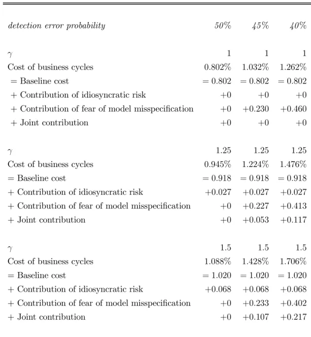
The consumption equivalent cost of business cycles is presented in Table 3. The table decomposes the cost into a contribution from idiosyncratic consumption risk and a contribution from an agent’s fear of model misspeciﬁcation. The decomposition starts from the baseline cost of business cycles when there is no idiosyncratic risk or fear of misspeciﬁcation. It is comparable to the Lucas calculation, obtained from the small noise expansion (5) by setting to zero both the variance of idiosyncratic shocks and the preference for robustness.6 _{The contribution of}

idiosyncratic consumption risk is isolated in the next row, which shows the additional cost of business cycles when there is idiosyncratic risk but no fear of misspecification. This is the case studied by De Santis (2007). The contribution of fear of model misspecification is in the next row, which is the additional cost of business cycles with a fear of misspecification but no idiosyncratic risk, the economy of Barillas et al. (2009). The cost of business cycles in Table 3 exceeds the sum of the baseline cost and the individual contributions from idiosyncratic risk and fear of misspecification. To complete the decomposition we therefore need an additional row, which measures the additional increase in the cost of business cycles when idiosyncratic risk and fear of misspecification operate jointly rather than separately.

That the combined effects of idiosyncratic consumption risk and fear of model misspeci-fication exceed their individual contributions is a central result of our paper. We find that introducing idiosyncratic risk significantly increases the cost of business cycles, even if agents are only slightly risk averse and have only a mild fear of model misspecification. For example, the consumption equivalent cost of adding idiosyncratic risk when γ = 1.5 is only 0.068% if the agent does not fear model misspecification, but this rises to 0.402% under a fear of model

6_{The cost of business cycles in Table 3 exceeds those calculated by Lucas (1987, 2003) because aggregate}

(12)

misspecification. We therefore argue that idiosyncratic risk can be costly even when risk aver-sion is much lower than that assumed by De Santis (2007). Symmetrically, endowing agents with a fear of model misspecification is more costly in an economy subject to idiosyncratic consumption risk. The Barillas et al. (2009) mechanism by which fears of model misspecifi-cation make business cycles costly is therefore amplified. We see that even a very mild fear of misspecification is sufficient to induce significant losses in consumption equivalent terms, for example when γ = 1.5the consumption equivalent cost of fearing model misspecification rises from 0.327% to 0.493% if there is idiosyncratic risk in the economy. If the data sample used in the calculation of detection error probabilities were less than 69 years then the costs would be higher.

(13)

detection error probability 50% 45% 40%

γ 1 1 1

Cost of business cycles 0.802% 1.032% 1.262%

= Baseline cost = 0.802 = 0.802 = 0.802

+ Contribution of idiosyncratic risk +0 +0 +0

+ Contribution of fear of model misspeciﬁcation +0 +0.230 +0.460

+ Joint contribution +0 +0 +0

γ 1.25 1.25 1.25

= Baseline cost = 0.918 = 0.918 = 0.918

+ Contribution of idiosyncratic risk +0.027 +0.027 +0.027

+ Joint contribution +0 +0.053 +0.117

γ 1.5 1.5 1.5

= Baseline cost = 1.020 = 1.020 = 1.020

+ Contribution of idiosyncratic risk +0.068 +0.068 +0.068

+ Joint contribution +0 +0.107 +0.217

Table 3: Decomposition of the consumption equivalent costs of business cycles

5.2 Interpretation

The force behind our result is that there is more for an agent to fear when it is subject to idiosyncratic risk. One part of this is that, as individual consumption becomes more volatile, the agent fears misspeciﬁcation not only of aggregate risk but also of idiosyncratic risk. Another aspect is that an agent might fear that aggregate and idiosyncratic risks may be interrelated. For example, it could be that aggregate and idiosyncratic shocks are correlated,

(14)

or that their variances co-move over time. A positive correlation between aggregate and idiosyncratic shocks is something to fear because it implies that the agent is more likely to suﬀer negative idiosyncratic shocks when the aggregate economy is doing badly. Co-movement between variances is similarly fear-inducing because it increases the likelihood that periods of idiosyncratic risk will occur against a backdrop of heightened aggregate risk.

Precisely how fears of model misspeciﬁcation translate into welfare losses is captured by the worst-case scenarios that agents construct to value alternative consumption streams. An agent fearing misspeciﬁcation distrusts its approximating model for the joint distribution of zt+1 ≡ (ct+1, δit+1). A worst-case conditional joint distribution of zt+1 is fˆ(zt+1) = m(zt+1)f(zt+1),

where f(zt+1) is the conditional density of zt+1 under the approximating model and mt+1

satisﬁes:

mt+1 ∝exp(−σβUt+1), (13)

where the factor of proportionality makes mt+1 have conditional mean one, i.e., it is the

reciprocal of the conditional mean of exp(₋σβUt+1). Ut+1 is an approximation to the value

function, in our case taken from the small-noise expansion (5). For a calibration of γ = 1.25

and detection error probability of 40%, Figure 2 plots contours of the normalised diﬀerence between the worst-case density and the density under the approximating model.7 _The

worst-case density has more probability mass than the density under the approximating model in the bottom left of the ﬁgure where the contours are positive. The opposite is true in the top right where the contours are negative.

7_{The diﬀerence in densities is normalised by dividing values of}_fˆ₍_zt+1)−f(zt+1)by the constant ( ˆf(zt+1)−

(15)

-0.8 -0.6 -0 .6 -0.4 -0.4 -0.2 -0.2 -0.2 0 0 0.2 0.2 0.₂ 0.4 0.4 0.6 0.6 0.8

√

₀

w

2t

√

0 w

1 t

-0.1

-0.05

0

0.05

0.1 -0.3

-0.2

-0.1

0

0.1

0.2

0.3

Figure 2: Diﬀerence in densities for γ = 1.25and 40% detection error probability. The worst-case density has more (less) probability mass than the density under the

approximating density where the contours are positive (negative).

Table 4 summarises the moments of the worst-case conditional consumption density for diﬀerent levels of risk aversion and detection error probability. The worst-case density diﬀers from the density under the approximating model in three respects. Firstly, it is centered on negative values of the aggregate consumption shock √ǫw1t and the idiosyncratic consumption

shock √ǫw2t. Secondly, it has slightly higher variances. Thirdly, the worst-case density has

greater probability mass than the density under the approximating model in the region where both aggregate and idiosyncratic shocks are negative. The characteristics of the worst-case density confirm the intuition that an agent with a preference for robustness fears negative shocks to aggregate and idiosyncratic consumption, and especially fears that these shocks may occur at the same time. Table 4 shows the degree to which these effects attenuate as the agent becomes less risk averse and less concerned with robustness. The covariance between aggregate and idiosyncratic shocks in the worst-case density tends to zero in the limit of either logarithmic utility or no fear of model misspecification.

(16)

detection error probability 50% 45% 40% γ 1 1 1 ˆ w1t 0 −0.240×10−3 −0.479×10−3 ˆ w2t 0 −2.850×10−3 −5.700×10−3 ˆ τ1 2.9% 2.9% 2.9% ˆ τ2 10% 10% 10% ρwˆ1,wˆ2 0 0 0 γ 1.25 1.25 1.25 ˆ w1t 0 −0.284×10−3 −0.525×10−3 ˆ w2t 0 −3.381×10−3 −6.245×10−3 ˆ τ1 2.9% 2.90011% 2.90019% ˆ τ2 10% 10.0085% 10.0080% ρ_w_ˆ1,wˆ2 0 0.250×10 −3 ₀_.₄₆₉_×₁₀−3 γ 1.5 1.5 1.5 ˆ w1t 0 −0.299×10−3 −0.532×10−3 ˆ w2t 0 −3.557×10−3 −6.315×10−3 ˆ τ1 2.9% 2.90022% 2.90041% ˆ τ2 10% 10.0092% 10.0171% ρ_w_ˆ₁_,_w_ˆ₂ 0 0.539_×10−3 ₀_.₉₉₅_×₁₀−3

(17)

6 Alternative consumption processes

The unit root processes for aggregate and idiosyncratic consumption in De Santis (2007) are key to generating sizeable welfare costs of aggregate fluctuations. Unfortunately, the empirical evidence for uninsurable unit roots in consumption is shaky. Blundell et al. (2008) find that many individuals are able to insure against permanent income shocks, whereas Heathcote et al. (2014) attribute only some of the fluctuations in consumption to unit root processes.

To investigate the sensitivity of our results to assumptions about consumption processes, we look at the consumption equivalent cost of business cycles when the unit roots are retained but the variance of idiosyncratic shocks is decreased by a factor of 2. Our aim is to produce a decomposition of welfare costs that can be compared directly to the numbers for γ = 1.5

and a detection error probability of 40% in the bottom right corner of Table 3. In doing the calculations, we therefore increase the preference for robustness parameter σ from 6.0 to 10.0. This reflects the greater difficulty an agent has distinguishing between models when the variance of idiosyncratic consumption shocks is low, and ensures that the detection error probability remains at 40%. The consumption equivalent cost of business cycles with a lower variance of idiosyncratic consumption shocks is 1.977%, which decomposes into a baseline cost of 1.020%, a contribution from idiosyncratic risk of 0.033%, a contribution from fear of model misspecification of 0.676% and a joint contribution of 0.247%. Although the magnitudes of the costs do fall slightly, we see that fear of model misspecification is again instrumental in making idiosyncratic risk increase the welfare cost of business cycles. Alternatively, introducing a fear of model misspecification is considerably more costly in an economy that is subject to idiosyncratic consumption shocks.

The consumption processes considered so far do not allow for a link between idiosyncratic risk and the aggregate state of the economy, a specification that may substantially understate the cost of business cycles. This is potentially important, as Storesletten et al. (2004) find that the cross-sectional income variation in the US is almost twice as high in contractions as in expansions. De Santis (2007) allows for such a link through a correlation between aggregate consumption shocks and the variance of idiosyncratic consumption shocks, but empirical work by Jacobsen et al. (1993) suggests that it is the increased risk and cost of job displacement that causes cross-sectional heterogeneity to rise during contractions. Specifically, job displacement probabilities and long-term earnings losses of job displacement go up in contractions. Indeed, in less formal discussions, the costs of recessions are often attributed to the increase in earnings losses of displaced workers during recessions, Davis and von Wachter (2011), or the earnings

(18)

losses for some sub-group of the population, Oreopoulos et al. (2014). In Krebs (2007) it has been shown that the welfare costs of business cycles become quite substantial once this particular feature is incorporated into the model.

We introduce job displacement risk by replacing the shock to the idiosyncratic component of consumption in (4) with the process of Krebs (2007):

w2t=            −dH with prob πpH pHdH 1−pH with prob π(1−pH) −dL with prob (1−π)pL pLdL 1−pL with prob (1−π)(1−pL) . (14)

The aggregate state of the economy is assumed to follow a stationary i.i.d. process, such that with probability π it is in expansion and with probability 1₋π it is in contraction. The probabilities of job displacement in expansions and contractions are pH and pL respectively,

with empirical evidence suggesting that pH < pL. If a worker is displaced then its individual

consumption level falls by dH if the economy is in an expansion and dL if the economy is

in a contraction, where it is assumed that dH < dL since earnings losses are typically lower

if a worker is displaced in an expansion than in a contraction. The increase in individual consumption of non-displaced workers is normalised so that the expected value of idiosyncratic consumption is not trending during either expansions and contractions.

Krebs (2007) measures the welfare cost of business cycles by the amount of consumption that agents would be willing to forego in order to live in an economy where both the proba-bility of job displacement and the consumption losses on displacement are constant over the business cycle. To ensure comparability across diﬀerent economies, the shock to idiosyncratic consumption when there is no cyclical variation in job displacement risk is modelled as:

¯ w2t= − ¯ d with prob p¯ ¯ pd¯ 1−p¯ with prob 1−p¯ (15) where p¯ = πpH + (1−π)pL and d¯= πdH + (1− π)dL. The consumption equivalent cost

of business cycles is the amount of extra consumption needed to compensate an agent for idiosyncratic consumption shocks following (14) rather than (15).

The i.i.d. nature of this formulation means that job displacement risk only aﬀects the model through changes in the moments of (w1t, w2t). The small noise expansion of Anderson

et al. (2012) hence remains valid and the calculations in Appendix A still apply. We adopt the numerical calibration of job displacement risk in Krebs (2007). The probabilities of job

(19)

displacement in expansions and contractions are set at pH = 0.03 andpL= 0.05respectively,

reﬂecting the lower likelihood of job displacement in an expansion than in a contraction. That workers lose 9% of their earnings if displaced during an expansion motivates setting

dH = 0.09. Similarly, job displacement in a contraction leads to a 21% loss of earnings and we

have dL = 0.21. Expansions and contractions are assumed to occur with the same frequency,

so π = 0.5. The numerical calibration implies that p¯ = 0.04 and d¯ = 0.15 in the model without cyclical variation in job displacement risk. The rest of the model is calibrated as in Section 4, with the coeﬃcient of relative risk aversion taking the value 1.5and the preference for robustness parameter σ chosen as before to generate detection error probabilities of 50%, 45% and 40% when testing based on a sample period of 69 years.

The welfare cost of a cyclical component in job displacement risk is decomposed at the top of Table 5. The story is similar to that in the previous model with no link between idiosyncratic risk and the aggregate economy, although now the consumption equivalent costs are larger. Looking at the final column for a detection error probability of 40%, we see that the cyclical component of job displacement risk raises the costs of business cycles by 0.153% if agents do not fear model misspecification, but by 0.446% if they do. Alternatively, endowing agents with a fear of model misspecification increases the costs of business cycles by only 0.615% if there is no cyclical component to job displacement risk, as opposed to 0.908% if there is.

(20)

detection error probability 50% 45% 40%

= Baseline cost = 1.022 = 1.022 = 1.022

+ Contribution of cyclical displacement risk +0.153 +0.153 +0.153

+ Joint contribution +0 +0.134 +0.293 ˆ π 0.5 0.49991 0.49970 ˆ pH 0.03 0.03001 0.03002 ˆ pL 0.05 0.05436 0.05953 E( ˆw1t|displaced in expansion) 0 −0.333×10−3 −0.699×10−3 E( ˆw1t|displaced in contraction) 0 −0.355×10−3 −0.743×10−3 E( ˆw1t|¬displaced in expansion) 0 −0.319×10−3 −0.666×10−3 E( ˆw1t|¬displaced in contraction) 0 −0.317×10−3 −0.664×10−3

Table 5: Decomposition of the consumption equivalent costs with job displacement risk The middle of Table 5 summarises the worst-case scenarios used by agents to value their consumption streams. The worst-case distribution has agents placing less probability mass

ˆ

π on the economy being in expansion, and more probability mass pˆH and pˆL on the risk of

job displacement. Agents especially guard against job displacement risk when the economy is in contraction, reflecting the greater loss of earnings they would suffer if displaced during a contraction. The bottom of Table 5 shows how fears of model misspecification inject correlation between the aggregate consumption shockwˆ1t and the cyclical component of job displacement

risk. The worst-case distribution of wˆ1t is always negative, but this is especially true if the

worker is displaced during a contraction. The agent therefore most fears that job displacement is likely to occur in both a contraction and when there is a negative aggregate consumption shock. The resulting correlation mirrors what we found between aggregate and idiosyncratic shocks in the worst-case distribution of the previous model .

(21)

7 Concluding remarks

The message that the welfare cost of business cycles is higher in an economy in which individ-uals face idiosyncratic consumption risk and are concerned about statistical model misspeci-fication should come as no surprise to readers of De Santis (2007) and Barillas et al. (2009). What might be more surprising is that the total effect of idiosyncratic risk and concerns about robustness exceeds the sum of their parts. Our calibration of the quantitative magnitude of the total effects offers additional support to the view that aggregate fluctuations are substantially more costly to individual consumers than calculated by Lucas (1987, 2003). The calculations of Lucas (2003) make no reference to whether business cycle fluctuations represent efficient allocations, but one conclusion from his estimates is that business cycles are not a worry be-cause costs are small even if all the fluctuations are departures from efficiency. We show that the cost of fluctuations is large, and hence it is important to understand the extent to which they are efficient.

A

The small noise expansion

Here, we outline how we apply a small noise expansion to obtain an approximate solution of value function recursion (1) in our economic environment. For details of the general case, see Anderson et al. (2012).

The ﬁrst step in expressing the right side of (7) in powers of√ǫis to expand the exponential expression over which an agent forms expectations through the operator Et. The Maclaurin

expansion for small √ǫ of this expression is:

e−σβ(W0₍_ci t+1)+h(c i t+1)) =e−σβ(W 0₍_ci t)+h(c i t)) 1 + ∞ n=1 ǫn/2_µ′ n n! (w1t+1+w2t+1) n _, µ′ n=κn+ n−1 m=1 n₋1 m₋1 κmµ ′ n−m, κn =−σβDn(W0(cit) +h(cit)), (16)

which is of the same form as the moment generating function of a random variable, with

µ′

n and κn analogous to the random variable’s non-central moments and cumulants. The

second step involves taking expectations of (16), applying logarithms, multiplying by ₋σ−1_,

and then making a Maclaurin expansion of the resulting expression for small√ǫ. When taking expectations of (16), the operator Et applies only to the expression (w1t+1+w2t+1)n, because

(22)

µ′

n is a deterministic function of the logarithm of individual consumption cit, which the agent

knows at time t. The result of the second step is an expression for the right side of (7) in terms of powers of √ǫ, as required:

βW0(ci_t) +βh(ci_t)₋ ∞ k=1 (₋1)k+1 kσ ∞ n=1 ǫn/2_µ′ n n! Et(w1t+1+w2t+1) n k . (17) We are now in a position to use the method of undetermined coeﬃcients to identify the correction term h(ci

t) in the small noise approximation. Substituting expression (17) into the

right side of (7) implies that the correction term satisﬁes:

(1₋β)h(ci_t) =₋ ∞ k=1 (₋1)k+1 kσ ∞ n=1 ǫn/2_µ′ n n! Et(w1t+1+w2t+1) n k . (18)

The way that √ǫ enters the right side of (18) directly through the expression ǫn/2 _and

in-directly through the dependency of µ′

n on κn, κn−1, . . . , κ1 and the derivatives Dn(W0(cit) +

h(cit)), Dn−1(W0(cit) +h(cit)), . . . , D(W0(cit) +h(cit))suggests that the correction term may be

written as a linear function of powers of√ǫ. A candidate is:

h(ci_t) =

∞

n=1

ǫn/2hn(ci_t), (19)

where the functionshn₍_ci

t)are independent of

√

ǫ. We verify the form of the candidate solution and identify its functions by applying the method of undetermined coeﬃcients to equations (18) and (19). The expected value Et(w1t +w2t)n is given by the moments of the bivariate

normal distribution of w1tandw2t. The method of undetermined coeﬃcients applied to terms

in √ǫ in (18) and (19) gives: h1₍_ci t) = Et(w1t+1+w2t+1) 1₋β βDW 0₍_ci t). (20)

There are no derivatives of h(cit) in the ﬁrst correction term (20) because h(cit) is at most of

order √ǫ. The second correction term is deﬁned by the undetermined coeﬃcients onǫin (18) and (19): h2(ci_t) = Et(w1t+1+w2t+1) 1₋β βDh 1₍_ci t) +Et(w1t+1+w2t+1) 2 2σ(1₋β) σβD 2_W0₍_ci t)− σβDW0(cit) 2 +(Et(w1t+1+w2t+1)) 2 2σ(1₋β) σβDW 0₍_ci t) 2 , (21)

(23)

where the derivativeDh1₍_ci

t)can be calculated from equation (20). This completes the

deriva-tion of the ﬁrst-order correcderiva-tion term√ǫh1₍_ci

t)+ǫh2(cit). An expansion of second order or higher

is obtained by recursive solution and application of the method of undetermined coeﬃcients to (18) and (19).

References

[1] Anderson, E., Hansen, L. and T.J. Sargent, 2003, A quartet of semigroups for model speciﬁcation, robustness, prices of risk, and model detection, Journal of the European Economic Association 1(1), 68—123.

[2] Anderson, E. W., Hansen, L.P. and T.J. Sargent, 2012, Small noise methods for risk-sensitive/robust economies, Journal of Economic Dynamics and Control 36, 468-500. [3] Atkeson, A. and C. Phelan, 1994, Reconsidering the Costs of Business Cycles with

In-complete Markets, NBER Macroeconomic Annual, Cambridge, MA: MIT Press

[4] Barillas, B., Hansen, L.P. and T.J. Sargent, 2009, Doubts or variability?, Journal of Economic Theory 144: 2388—2418.

[5] Beaudry, P. and C. Pages, 2001, The Cost of Business Cycles and the Stabilization Value of Unemployment Insurance, European Economic Review 45(8): 1545-1572.

[6] Blundell, R., Pistaferri, L. and I. Preston, 2008, Consumption Inequality and Partial Insurance, American Economic Review 98(5): 1887—1921.

[7] Davis, S.J. and T.M. von Wachter, 2011, Recessions and the Cost of Job Loss,Brookings Papers on Economic Activity 43(2): 1-72.

[8] De Santis, M., 2007, Individual Consumption Risk and the Welfare Cost of Business Cycles, American Economic Review 97(4): 1488-1505.

[9] Hansen, L.P. and T.J. Sargent, 2001, Robust Control and Model Uncertainty, American Economic Review 91(2): 60-66.

[10] Hansen, L.P. and T.J. Sargent, 2008, Robustness, Princeton, New Jersey, Princeton Uni-versity Press.

(24)

[11] Hansen, L.P. Sargent, T.J. Turmuhambetova, G.A. and N. Williams, 2006, Robust Con-trol, Min-Max Expected Utility, and Model Misspeciﬁcation,Journal of Economic Theory 128: 45-90.

[12] Hansen, L.P., Sargent, T.J. and N.E. Wang, 2002, Robust permanent income and pricing with ﬁltering, Macroeconomic Dynamics 6, 40—84.

[13] Heathcote, J., Storesletten, K. and G.L. Violante, 2014, Consumption and Labor Supply with Partial Insurance: An Analytical Framework, American Economic Review, forth-coming.

[14] Jacobson, L.S., LaLonde R.J. and D.G. Sullivan, 1993, Earnings Losses of Displaced Workers, American Economic Review 83(4): 685-709.

[15] Krebs, T., 2007, Job Displacement Risk and the Cost of Business Cycles, American Economic Review 97(3): 664-686.

[16] Lucas, R. E., 1987, Models of Business Cycles, New York: Blackwell

[17] Lucas, R. E., 2003, Macroeconomic Priorities, American Economic Review 93(1): 1-14. [18] Oreopoulos, P., T.M. von Wachter and A. Heisz, 2012, The Short- and Long-Term Career

Eﬀects of Graduating in a Recession: Hysteresis and Heterogeneity in the Market for College Graduates, American Economic Journal: Applied Economics 4(1), 1-29.

[19] Tallarini, T. D., 2000, Risk-sensitive real business cycles,Journal of Monetary Economics 45(3): 507-532.