Statistical-thermodynamical analysis, using Tsallis statistics, in high energy physics

University of Cape Town

Statistical-thermodynamical analysis, using Tsallis

statistics, in high energy physics

by

Andile Whitehead

Submitted to the Department of Physics

in fulfillment of the requirements for the degree of

Master of Science in Theoretical Physics

at the

UNIVERSITY OF CAPE TOWN

2014

c

University of Cape Town 2014. All rights reserved.

Author . . . .

Department of Physics

Certified by . . . .

Jean Cleymans

Professor

Thesis Supervisor

Accepted by . . . .

Chairman

Chairman, Department Committee on Graduate Theses

The copyright of this thesis vests in the author. No

quotation from it or information derived from it is to be

published without full acknowledgement of the source.

The thesis is to be used for private study or

non-commercial research purposes only.

Published by the University of Cape Town (UCT) in terms

of the non-exclusive license granted to UCT by the author.

Statistical-thermodynamical analysis, using Tsallis statistics,

in high energy physics

by

Andile Whitehead

Submitted to the Department of Physics in fulfillment of the

requirements for the degree of Master of Science in Theoretical Physics

Abstract

Obatined via the maximisation of a modified entropy, the Tsallis distribution has been used to fit the transverse momentum distributions of identified particles from several high energy experiments. We propose a form of the distribution described in [1] and show it to be thermodynamically consistent. Transverse momenta distri-butions and fits from ALICE, ATLAS, and CMS using both Tsallis and Boltzmann distributions are presented. Tsallis fits were found to fit theptspectra extremely well

when compared to the associated Boltzmann fits. Unfortunately universal parameters for the temperature,T, the nonextensivity parameter, q, and the fireball radius, R, could not be maintained; however, the prospect of obtaining such values, and conse-quently deriving relations for q and T at varying energy, √s, measured in the centre of momentum frame, appears promising.

Thesis Supervisor: Jean Cleymans Title: Professor

Acknowledgments

Thank you to Professor Jean Cleymans and Dr. Danish Azmi without whose help this would not have been possible.

Contents

1 Introduction 12

1.1 Quantum Chromodynamics (QCD) . . . 13

1.1.1 Quarks, Gluons and Colour Charge . . . 13

1.1.2 The Strong Potential and Colour Confinement . . . 16

1.1.3 Asymptotic Freedom . . . 17

1.1.4 Quark Gluon Plasma (QGP) . . . 18

1.2 Statistical Thermodynamic Models . . . 22

2 Boltzmann-Gibbs Statistics 23 2.1 Quantum Statistics . . . 27

3 Tsallis Distribution 31 3.1 Micro-Canonical Ensemble . . . 34

3.2 Canonical Ensemble . . . 36

3.3 Grand Canonical Ensemble . . . 38

3.4 Thermodynamic Consistency . . . 43

4 Results 54

5 Discussion 68

6 Conclusion 73

B Kinematics 78

B.1 Rapidity and pseudorapidity . . . 78 B.2 Pressure in a non-interacting gas . . . 80

List of Figures

1.1 Baryon octet with JP ₌ 1 2 +

.Particles along the same horizontal line share the same strangeness number, S, those along the vertical the same isospin, I3 , and those on the same diagonals share the same

charge,Q[2]. (Image sourced from http://en.wikipedia.org/wiki/File:Baryon octet.png) 14 1.2 The relevant attributes of particles in the Standard Model [2]. (Image

sourced from http://en.wikipedia.org/wiki/File:Standard Model of Elementary Particles.svg). . . 15 1.3 Graphic displaying the difference between the strong potential, Vs

be-tween individual quarks and the modified strong potential, VD due to

the Debye screening of the partonic medium. The dashed line repre-sents the Debye length, rD of the medium. . . 19

1.4 QCD phase diagram for strongly interacting matter [3] . . . 20

4.1 Graph, obtained from [4], of particle ratios taken from several experi-ments at 200 GeV. . . 55 4.2 Tsallis and Boltzmann fits to pt spectra for ALICE pp experiment

performed at 900GeV for π+_{(left panel) and π}−_{(right panel) mesons.}

Refer to (4.1) for Tsallis parameter values. . . 60 4.3 Tsallis and Boltzmann fits to pt spectra for ALICE pp experiment

performed at 900GeV for K+(left panel) and K−(right panel) mesons. Refer to (4.1) for Tsallis parameter values. . . 61

4.4 Tsallis and Boltzmann fits to pt spectra for ALICE pp experiment

performed at 900GeV for p(left panel) and ¯p(right panel) baryons. Refer to (4.1) for Tsallis parameter values. . . 61 4.5 Tsallis and Boltzmann fits to pt spectra for ALICE pp experiment

performed at 900GeV for Λ(left panel) and ¯Λ(right panel) baryons. Refer to (4.1) for Tsallis parameter values. . . 62 4.6 Tsallis and Boltzmann fits topt spectra for ALICE pp experiment

per-formed at 900 GeV forφmeson(left panel) and Tsallis and Boltzmann fits toptspectra for ALICE pPb experiment performed at 5020 GeV for

charged particles(left panel). Refer to Table(4.1) for Tsallis parameter values. . . 62 4.7 Tsallis fit to pt spectrum for ALICE pp experiment performed at

900GeV for proton, with q value for Tsallis fit fixed to the q = 1.129 value obtained from the antiproton spectrum. Fit values obtained for the two remaining parameters were T = 0.0553±0.0044 GeV and

R= 6.8±1.2 GeV−1 and χ2_{/NDF = 7.71675/22. . . . 63}

4.8 Tsallis fit to pt spectra for π+, π−, K+, K−, p, ¯p, Λ, Λ and¯ φ particles

for ALICE pp experiment at 900 GeV. (Anti)Particle fits are shown as (dashed)solid lines. . . 63 4.9 Tsallis fit topt spectra for π+, π−, K+, K−, p and ¯p particles for CMS

pp experiment at 900 GeV. (Anti)Particle fits are shown as (dashed)solid lines. . . 64 4.10 Tsallis fit toπ+_{, π}−_{, K}+_{, K}−

, p and ¯p particles for CMS pp experiment at 7 TeV. (Anti)Particle fits are shown as (dashed)solid lines. . . 64 4.11 Calculated fireball radii for several particle spectra obtained from

AL-ICE, CMS and ATLAS experiments at varying energies (Proton radius does not appear in graphic as including would have compromised the scaling). . . 65 4.12 Calculated fireball temperatures for several particle spectra obtained

4.13 Calculated fireball q values for several particle spectra obtained from ALICE, CMS and ATLAS experiments at varying energies. . . 66 4.14 Contour plots of the multinormal probability density, for ALICE pp

collision at 900 GeV, for proton. Left panel shows invertedχ2_{values as}

a function of (T, q) with R fixed at R = 28 GeV−1. Right panel shows inverted χ2 _{values as a function of (T, R) withq fixed at q= 1.1543. . 66}

4.15 Contour plots of the multinormal probability density, for ALICE pp collision at 900 GeV, for proton (left panel) and antiproton (right panel) . Left panel shows inverted χ2 values as a function of (q, R) with T fixed at T = 0.056 GeV. Right panel shows inverted χ2 _values

as a function of (q, T) withR fixed atR = 6.5 GeV−1. . . 67 4.16 Contour plots of the multinormal probability density, for ALICE pp

collision at 900 GeV, for antiproton. Left panel shows inverted χ2

values as a function of (T, R) with q fixed at q = 1.129. Right panel shows inverted χ2 values as a function of (q, R) with T fixed at T = 0.056 GeV. . . 67

List of Tables

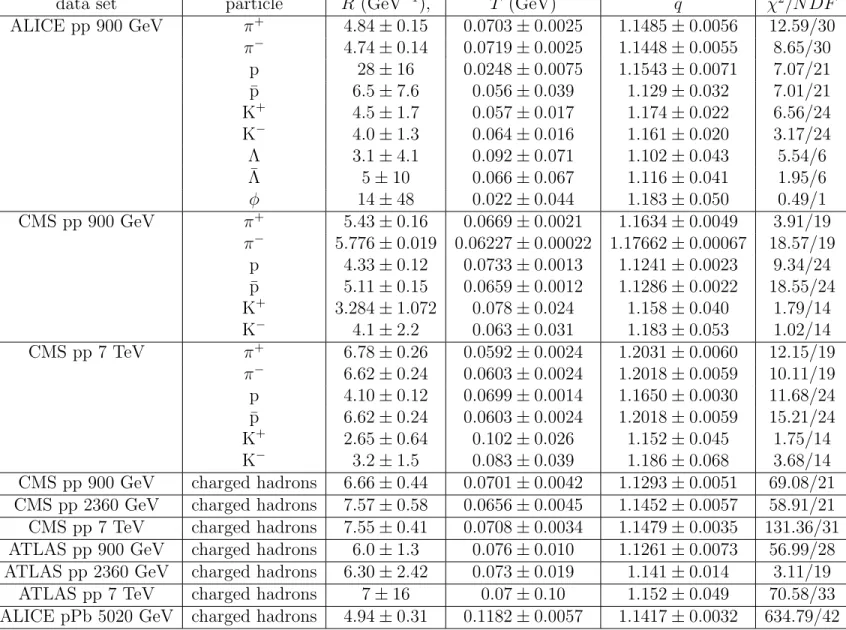
4.1 Parameter and χ2/N DF values obtained from Tsallis fits performed on ALICE, CMS and ATLAS data sets at several energies, whereR is the fireball radius,T the fireball temperature, andq the Tsallisq value. 59 4.2 Correlation coefficients for fitted parameters for several hadrons from

Chapter 1

Introduction

Since the advent of humanity, Man has possessed an innate curiosity. It is perhaps this nature of inquiry, that has been the primary driving force for the immense progress the human species has come to enjoy. Despite His extensive knowledge, Man still remains incapable of satisfactorily answering the essential questions posed by exis-tentialism. Among these is that of:“Of what is nature fundamentally comprised?”. The notion that all visible matter is derived from a finite set of elements was intro-duced by the ancient Greeks. They considered earth, water, fire and air to be the fundamental constituents of nature. However, with the development of chemistry it appeared that there were significantly more of these indivisible elements than the ancient Greeks had initially proposed. In 1869, the Russian chemist and inventor, Dmitri Mendeleev, published the periodic table of elements in which he categorised the fundamental elements of nature. For many decades scientists considered the pe-riodic table to represent the ultimate reduction of nature into its basic constituents. However, in 1911, this view was dispelled with Rutherford’s gold foil experiment in which he bombarded a strip of gold foil with alpha particles. Due to the peculiar na-ture with which the alpha particles were deflected from the gold strip, it was apparent that the atom could not possibly be comprised of electrons “floating” in a uniform distribution of positive charge, as suggested by the then popular plum-pudding model; instead, the atom had to possess some further internal structure with a localised pos-itively charged nucleus surrounded by negatively charged “orbiting” electrons. It was

later discovered that the nucleus consisted of positively charged protons and neu-trally charged neutrons. With this it appeared that physicists had finally succeeded in describing the principle constituents of matter. However, more remarkable findings were still on the horizon. The short-range strong force, required to bind the nucleons, inspired the Japanese physicist Hideki Yukawa to introduce the pion as the boson mediating this interaction, after which he proposed that experimentalists should look for the particle. Indeed, in 1947, the pion was found by analysing cosmic-ray radi-ation and with the dawn of particle accelerators, a plethora of strongly interacting subatomic particles, collectively known as hadrons, were discovered. In 1964, the quark model was postulated independently by the physicists Murray Gell-Mann and George Zweig, in order to provide an ordering scheme for the categorization of the proliferation of hadrons that were being discovered in the then high energy experi-ments. The model was considered purely as a method for categorizing hadrons, and not as a representation of some physical configuration within the hadrons. However,it soon became clear that the quark model was more than a tool for ordering hadrons and was in fact a physical representation of the structure of hadrons. These findings led to the establishment of the Standard Model (SM) of matter for describing the fundamental particles and force carriers in nature. Currently the SM model appears to best describe the fundamental composition of all visible matter and the interac-tions of these fundamental particles. Much is still unknown about the dynamical interactions of these fundamental particles and much research is still required to fully illuminate the nature of this complex subatomic world.

1.1

Quantum Chromodynamics (QCD)

1.1.1

Quarks, Gluons and Colour Charge

As described previously the quark model was independently proposed in 1964 by Gell-Mann [5] and Zweig [6] as a means to categorize the plethora of hadrons being discovered at the time. Groups, or multiplets, of baryons and mesons display a certain

orderliness in their internal quantum numbers and can be fit into geometrical patterns according to their isospin and their strangeness [7]. As a result of the quark model

Figure 1.1: Baryon octet withJP ₌ 1 2 +

.Particles along the same horizontal line share the same strangeness number, S, those along the vertical the same isospin, I3 , and

those on the same diagonals share the same charge, Q [2]. (Image sourced from http://en.wikipedia.org/wiki/File:Baryon octet.png)

it was realised that these geometrical arrangements of hadrons are derivative of their internal quark constituents. In the current, view the quarks are categorised into three generations, each of which contain two quarks as displayed in fig(1.2). The down (d), strange (s) and bottom (b) quarks carry an electric charge of −1

3 while the up (u),

charm (c) and top (t) carry +2₃ . All quarks are fermions with spin 1₂ and under regular temperatures and pressures are always found in hadron bound states. These bound states can exist in one of two forms, namely, mesons or baryons. Mesons are comprised of a quark-antiquark pair (qq¯), and baryons, consist of three quarks (qqq) or three antiquarks (¯qq¯q¯). While baryons possess half integer spin and consequently obey Fermi-Dirac statistics, mesons on the other hand are integer spin hadrons and thusly adhere to Bose-Einstein statistics respectively.

It later became apparent that a further intrinsic degree of freedom had to necessarily be associated with each quark. This SU(3) (anti-symmetric) degree of freedom

at-Figure 1.2: The relevant attributes of particles in the Standard Model [2]. (Im-age sourced from http://en.wikipedia.org/wiki/File:Standard Model of Elementary Particles.svg).

tributable to each quark, was known as colour charge. The notion of colour charge is analogous to that of electric charge; the primary difference being that three types of colour charge exist, namely, red, green, blue, along with their corresponding “neg-ative” anti-red, anti-green and anti-blue charges appropriately associated with the antiquarks. By virtue of the fact that hadrons possessing a non-zero colour charge have not been observed in nature, the natural conclusion would thus be that the strong force must act in such a way as to ensure that the bounded quarks (along with the gluons) within the hadron exist as a combined colourless SU(3) singlet state. A combination of red, green and blue, or anti-red, anti-green and anti-blue quarks forms a colourless baryon state while an oppositely colour-charged quark-antiquark pair (e.g. red and anti-red) forms a colourless meson state.

1.1.2

The Strong Potential and Colour Confinement

The strong interaction is mediated by the set of eight gluons (forming a colour octet) that couple to colour charge1. The strong potential,Vs , between two opposite colour

charges, can be modelled by [7]:

Vs =−

4 3

αs

r +kr (1.1)

wherer is the distance between the charges, αs is the coupling constant of the strong

interaction andk is the string tension, a factor representing the strength of the quark binding force. At short distances the first term in (1.1) dominates the behaviour of the potential, diminishing like ∼ 1

r with increasing distance similar to the Coulomb

potential. Perhaps somewhat less intuitively: as the distance, r, between the charges increases, the second term in (1.1) dominatesVsand gives rise to the linear behaviour

of the potential at larger. This has the implication that an infinite amount of energy is required to free a quark. It is this particular property of the strong interaction, appropriately termed confinement, that explains why free quarks or colour-charged hadronic states have never been observed.

In QCD, the colour-confining nature of the strong interaction is attributable to the fact that gluons carry colour charge; consequently, unlike the electrically neutral photons, they are able to couple to one another. When the separation between two quarks exceeds ∼ 1 fm, the gluon-gluon coupling begins pulling the colour field lines together into string-like objects. At large enough distances it becomes more energetically favourable to create a quark-antiquark pair from the vacuum rather than further extending the length of the string.

1_{The ninth gluon forms a colourless singlet state and so does not participate in the strong}

1.1.3

Asymptotic Freedom

The strong coupling constant αs in (1.1), derived in Quantum Field Theory (QFT),

essentially, was determined in order to quantify the strength of the strong interaction. Deceptively, αs is not in fact a constant at all, but rather a function of the separation

between the charges,r, or the four-momentum exchange,q2. Evidently, high momen-tum transfers are associated with short range interactions and vice versa and so the dependence ofαs onq2 necessarily implies the dependence ofαs onr. The variability

of the strong coupling constant, is referred to as the running coupling strength; the underlying cause for which (amongst other things) lies in the quantum fluctuations of the vacuum. Uncertainty Principle. Analogous to vacuum polarisation in QED, a colour charge can polarise the surrounding virtual quark-antiquark pairs that are created (and annihilated) by the vacuum. As a result, the polarised vacuum partially screens the colour charge, and thus reduces the magnitude of its field. However, in addition to the vacuum polarisation generated by the virtual quark pairs, an addi-tional effect is observed: Gluons are able to couple to the exchange gluons associated with the virtual quark pairs and ultimately form a cloud of self-interacting gluons around the virtual quarks which has the peculiar effect of producing a conflicting, anti-screening effect.

Using the renormalisation technique, the strong coupling constant αs(|q2|) at a

given momentum transfer, q2 _{, can be expressed in terms of a measured α}

s(|q02|) at

a particular q2 = q₀2 . The relation describing the dependence, or “running”, of the strong coupling constant with respect to q2_{, as derived from QCD, is [7]:}

αs(|q2|) =

12π

βln (|q2_|/Λ2₎ (1.2)

where Λ is the QCD scale constant, a parameter determined experimentally via mea-suring αs at different q2 values. Typically quoted values of Λ are of the order of

∼200 MeV. The counteracting effects of the quark and gluon polarisation in creating an overall screening or anti-screening effect is controlled by the β term in (1.2). The

simple formula describing β is:

β = 11n−2f, (1.3)

where f and n are respectively, the postulated number of quark flavours and colour charges that occur in nature. In the theory, if 11n > 2f then the anti-screening effect due to the gluon-gluon coupling will dominate the screening effect of the vir-tual quark pairs and the effective coupling will decrease with increasing q2. Given that there are six quark flavours and three colour charges in the theory (β = −21) this will evidently be the case. Due to the inverse correlation between r and q2, we can equivalently state that, at short distances, the strong force effectively becomes relatively weak. This characteristic of the strong interaction is termed asymptotic freedom. The phenomenon of asymptotic freedom provides a regime in which ana-lytical calculations for experimental observables can be performed: In the regime of high momentum transfer, whereq2 _>>Λ2 _{, the coupling constant tends to zero. This}

fortuitous property of the coupling constant allows for the use of perturbation theory in QCD, [8], to make experimentally verifiable predictions, for relevant observables.

1.1.4

Quark Gluon Plasma (QGP)

Phases of Strongly Interacting Matter

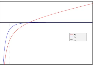
Naturally, the discovery of asymptotic freedom led to speculation of a possible phase transition from partons existing within bound states of hadronic matter to a decon-fined state of partons, the quark gluon plasma (QGP) [9]. Evidently, two interacting quarks situated within close proximity of one another (alternatively, large q2), can be in a temporary state of asymptotic freedom. However, the existence of a QGP, necessitates the existence of a medium of quarks and gluons where individual partons are able, uninhibitedly, to traverse distances larger than the typical size of hadronic states. Evidently, (1.1) does not include the effects of the medium, i.e. the plasma, on the potential between the two opposite colour charges. It is this presence of numer-ous mobile colour charges in the QGP, that results in the screening of individual long

Radius (r) Potential s V D V D r

Figure 1.3: Graphic displaying the difference between the strong potential,Vsbetween

individual quarks and the modified strong potential, VD due to the Debye screening

of the partonic medium. The dashed line represents the Debye length, rD of the

medium.

range interactions, known as Debye screening. Considering only the short range term of the QCD potential (first term in (1.1)), the presence of Debye screening modifies the potential such that:

Vs(T, r)∼ −

αs

r e

− r

rD _(1.4)

where T is the temperature of the plasma and rD(T) is the temperature dependent

Debye length, which characterises the length from which the potential is screened2_.

When rD becomes smaller than the typical radius of a hadron the strong force no

longer confines the partons and the bound state dissolves. Thus, in addition to the attenuation of the coupling constant with decreasing r, increasing the density of colour charges has the effect of screening the long range influence of the strong potential. The increased density can be achieved via thermal excitation or extreme compression of a hadronic system. Consequently, the formation of a highly dense system in combination with a small coupling constant are the conditions necessary

for the occurrence of the phase transition from a state of hadronic matter to that of the QGP. Non-perturbative methods, such as Lattice QCD, have been used to gauge the critical temperature, TC, and energy density, C, at which such phase

transitions occur. These calculations estimateTC to be in the range 155−160 MeV and

C ∼1 GeV/fm3 [10]. The relation between the energy density and the temperature,

derived from the Stefan-Boltzmann (SB) law for the case of low net baryon density (µB ∼0), is [11]: T4 = 2(n2_c−1) + 2ncnf 7 4 π2 30 (1.5)

wherenf andncare the respective number of quark flavours and colour charges. The

fact that the energy density lies below the SB limit indicates that quarks still undergo interactions and asymptotic freedom is not achieved, at least for T < 4TC . In the

QGP, quarks become deconfined and their mass drops down from the dynamical value within a hadron, of the order of ∼300 MeV (for u and d quarks), to the bare value of ∼ 5MeV.

Fig(1.4) shows a sketch of the phase diagram of strongly interacting matter in (µB, T)

, GeV µB T, GeV 1 0 nuclear 0.1 CFL QGP E critical point

vacuum matter quark matter quark matter

Figure 1.4: QCD phase diagram for strongly interacting matter [3]

parameter space, where the baryon chemical potential,µB, is essentially a measure of

the asymmetry between quarks and antiquarks in the system. “Cold” nuclear matter, such as typical nuclei, occur at low T and µB ∼900 MeV. When excited thermally,

hadrons, primarily pions, are produced and begin to occupy the space between the nucleons. When the hadron gas that has formed is sufficiently heated or compressed, the medium attains a density sufficiently large for the effects of Debye screening to be experienced within regions of the hadron gas. Consequently, in and amongst the hadronic matter, regions of free partons form, which at the critical temperature, TC,

spreads throughout the entire volume of the hadron gas. The phase boundary with the QGP state is represented by the solid line in fig(1.4). If matter is only compressed, increasing µB while keeping the temperature of the system relatively low, the phase

transition is located on the right side of the diagram. Based on different models the two phases are separated by a line of constant energy density across which the transition is of first order. However, according to Lattice QCD calculations, a certain critical point is reached asµB→0, beyond which the transition is expected to become

a rapid crossover. This is the region which is experimentally accessible in heavy-ion collisions at the SPS, RHIC and LHC, going to lower and lower µB as the

centre-of-mass energy of the collisions increases. At µB ∼ 0, along the line where the early

universe evolved, the transition is predicted to happen at a critical temperature of

TC ≈160 MeV.

Ultra-relativistic heavy-ion collisions are used to probe the lowµB and highT region

of the QCD phase diagram where matter is predicted to exist in the QGP phase. The QGP formation is not observed directly, but by studying the final state of the interactions, looking for particular signatures which are expected only in systems where the QGP is produced, such as central A-A (i.e. nucleus-nucleus) collisions, and are less likely to occur in others such as p-p (proton-proton) or peripheral A-A. For this reason analyses are usually done on both A-A and p-p data in order to establish if a particular observable is due to the QGP formation (or compare A-A with different collision centralities).

1.2

Statistical Thermodynamic Models

Due to the running nature of the strong coupling constant, αs, QCD is only

per-turbative within certain energy regimes, specifically, large q2_{; however, in the low}

energy regime, due to the magnitude of αs, the perturbative methods of QCD are

inapplicable. Thus, describing low energy phenomena in QCD has necessitated the development of phenomenological models, of which there are numerous. Amongst these, thermal models are widely used and have proven to be extremely successful in reproducing experimental results for various quantities measured in heavy-ion col-lisions [12], [4]. Essentially, the simplest statistical-thermal models, are those that model the hadrons produced during the heavy-ion collision as a gas of non-interacting particles. When one uses such statistical models an important assumption is that the system being treated reaches equilibrium i.e. equilibrium distributions are assumed. It is extremely peculiar that such models should perform so well given that the sys-tem at chemical freeze-out (cessation of inelastic collisions) has insufficient time to equilibrate through rescattering (kinetic thermalisation); yet somehow the results ob-tained for the hadron yields using such models are consistent with those obob-tained experimentally. This raises theoretical questions about the possible statistical nature of the hadronization process.

Chapter 2

Boltzmann-Gibbs Statistics

In this section we shall briefly describe the formulation of typical statistical mechanics used in the, non-interacting hadron gas, models used to describe the particles gener-ated in heavy-ion collisions.

When two heavy-ions collide they produce what is known as a fireball. In the primor-dial fireball numerous hadrons are created. In such high energy interactions, particle numbers are not conserved. However, it is known that such interactions do conserve the initial quantum number content of the interaction. This argument, distinctly ignores weak interactions. This is quite a valid assumption, since the relevant time scales are usually considerably shorter than the typical times scales for weak inter-actions which are typically between 11-15 orders of magnitude longer than strong interactions. Thus, when modelling the system statistically; instead of conserving particle numbers - as one would typically do - it is the initial quantum number con-tent of the system that is conserved. However, in practice, this is not as trivial as one may assume [4]. The degree of stopping of the colliding nuclei, is evidently dependent on the beam energy, and this clearly affects the choice of baryon number and charge. Furthermore, the centrality of the collision also affects the quantum number content. The quantum numbers usually conserved when performing these calculations are baryon number, B, charge, Q, and strangeness, S and occasionally charm, C. Top-ness, T, and bottomnessbare usually not included as it is reasonable to assume that such heavy quarks are very rarely produced (at these energies). Thus the chemical

po-tential associated with a particular hadron species,i, in the hadron gas at freeze-out is given byµi =µbBi+µQQi+µSSi+µCCi, whereµB, µQ, µS, µC are, respectively, the

chemical potentials associated with baryon number, charge, strangeness, and charm of the system. Evidently, the net quantum number content of the system is given by:

B =X i BiNi 0 = X i SiNi Q= X i QiNi 0 = X i CiNi, (2.1)

whereNi is the number of particles of specieiin the hadron gas, and the sum in (3.1)

is taken over both particles and anti-particles.

When implementing a statistical-thermal analysis of a chosen system it is necessary that one decides in which ensemble to operate [13], the choice of which largely de-pends on one’s desired treatment of the conservation laws. There are three statistical ensembles, namely, the micro-canonical (MCE), canonical (CE) and grand canonical (GCE) ensembles that are used extensively. Of these, the MCE is the most restrictive, in that the energy and the quantum numbers in such ensembles are fixed precisely. Somewhat less restrictive is the CE in which relevant quantum numbers remain fixed but the energy; however, is set on average by the temperature,T, of the system. That is to say; if one were to measure the total energy of the system numerous times, these calculated energies would fluctuate around the average energy of the system (deter-mined by the temperature). In the GCE, both the energy and quantum numbers, respectively, are set on average by the temperature, T, and the chemical potential/s

µi, whereirepresents some conserved quantum number. With the appropriate choice

of ensemble, one’s task is to compute the partition function of the system under con-sideration. Once evaluated, the partition function can be utilised to calculate the relevant thermodynamic quantities characteristic of the fireball at freeze-out.

Generally, in the GCE, the partition function is derived via considering the transfer of energy and particles between a system and a large reservoir. We can obtain the same probability distribution function via the extremization of the Shannon-Gibbs

entropy [14] given by: S =− W X i pilnpi, (2.2)

where the index i labels each unique configuration (microstate) of the system and

W ∈_Nrepresents the total number of possible configurations of the system, with the constraints, f({pi}) = W X i pi = 1, (2.3) g({pi}) = W X i Eipi = ¯E, (2.4) h({pi}) = W X i Nipi = ¯N . (2.5)

From information theory, entropy is a measure of our knowledge of the state of a system, where S1 = 0 describes perfect knowledge of the state of the system. Thus

given the constraints in (2.3-2.5) we seek to maximize the entropy, i.e. make the least biased estimate of our system given the limited information provided. When maximising a multivariable functional subject to a given number of constraints, the approach used is that of the method of Lagrange multipliers. Consequently, the variational problem that requires solving is:

δ[S({pi})−αδf({pi})−βδg({pi})−γδh({pi})] = 0, (2.6)

where α, β, γ ∈ _R. Evidently (2.6) is merely a compact form of expressing W equa-tions of the form:

where {n ∈_N|n∈ [1, W]}. (2.7) simplifies to the following expression for the proba-bilities of the various states of the system at equilibrium:

pn =Ae−(βEn+γNn), (2.8)

where1 A= exp{−α−1}. Moreover, the constraint expressed in (2.3) allows for the reformulation of A into the following :

A= X

i

e−(βEi+γNi)

!−1

. (2.9)

Describing the system in terms of its possible macrostates (as opposed to microstates), (2.9) can be reformulated into the more familiar form:

A= ∞ X N=0 X i e−(βEi+γN) !−1 , = 1 ZGC , (2.10)

where the index i now represents the macrostate (defined solely by the energy and not the number of particles of the system) with energy Ei, and N the number of

particles (which is run over for each particular macrostate). Hence, we can identify

A= 1/ZGC whereZGC is the partition function of GCE by identifying the parameters

β = _T1 and γ = βµ. Evidently, we have derived the probability distribution func-tion for the GCE at equilibrium via the extremizafunc-tion of the SG entropy under the constraints expressed in (2.3)-(2.5), under purely statistical, non-physical, arguments.

1_{Evidently, this is under the assumption that a configuration is uniquely determined by its energy}

2.1

Quantum Statistics

If the given system is quantum mechanical, then it will be composed ofαenergy levels

ν each with a given number of particles nν, such that Pnνν =En and Pnν =N.

Using this new prescription, the GC partition function is given by:

ZGC = ∞ X N ∗ X {nν} Y ν e−β(νnν−µnν) _(2.11) = X {nν} Y ν e−β(νnν−µnν) _(2.12) where P {nν} = P n1 P n2. . . P

nα and the asterisk in (2.11) is representative of the

constraint: P

nν =N. Consequently, one can then rewrite (2.12) as:

ZGC = X {nν} Y ν e−β(ν−µ)nν _(2.13) ZGC = Y ν zν, (2.14)

where zν is the partition function for the νth energy level. If the system is composed

of fermions then {nν ∈N0|n∈[0,1]}. Resultantly:

zF D_ν = 1 +e−β(ν−µ)_{. (2.15)}

If, instead, the system is comprised of bosons, the partition function for energy level

ν is given by: zBE_ν = ∞ X nν=0 e−β(ν−µ)nν_{, (2.16)} = 1 1−e−β(ν−µ). (2.17)

The average population number of a given quantum state will be given by: hnνi= P∞ nν=0nνe −β(νnν−µnν) P∞ nν=0e −β(νnν−µnν) , (2.18) =−1 β ∂lnzν ∂ν , (2.19)

which in the case of fermions and bosons is given by:

hnνi F D,BE

= 1

eβ(ν−µ)±1, (2.20)

where the plus and minus signs denote the average occupation number for fermions and bosons respectively.

Since the average number of particles is given by:

N =−∂Ω ∂µ =T∂lnZ GC ∂µ =±T∂ P νln 1±e −β(ν−µ) ∂µ =X ν e−β(ν−µ) 1±e−β(ν−µ) =X ν hnνi (2.21)

We can now multiply and divide by a factor of ∆pi, but since ∆pi = 2π/Li(quantum

mechanical particle in a box with continuous boundary conditions) where i=x, y, z

we can rewrite (2.21) as ¯ N =X ν V (2π)3 hnνi(∆px)(∆py)(∆pz) (2.22)

where V =Q

iLi. Taking the limit where Li → ∞(the large volume approximation)

we find that the average number of particles is given by:

¯ N =V Z _d3_p (2π)3hnip, =V Z _d3_p (2π)3 1 eβ(−µ)_±1. (2.23)

Using the above result, it can be easily shown that the entropy for a gas of identical fermions/bosons is given by 2_:

SF D,BE =−X

ν

[nνlnnν ±(1∓nν) ln (1∓nν)]. (2.24)

Evidently3, in the Boltzmann limit, i.e. an ideal gas of extremely low concentration or high temperature, the expression for the average occupation number expressed in (2.20) reduces to:

hnνiB =e−β(ν−µ). (2.25)

Thus, using the expression for the Boltzmann approximation for the mean occupation number in (2.21), the expression for the entropy in (2.24), in the Boltzmann limit, simplifies to:

SB =−X

ν

[nνlnnν −nν]. (2.26)

One can show naturally in an analogous manner to the previous analysis that the maximization of this particular entropy with respect to the constraints:

g =X ν nνν = ¯E, (2.27) h=X ν nν = ¯N , (2.28)

2_{This is shown in appendix A.} 3_{The notationn}

reproduces the expression for the approximated average occupation number in (2.21), and so ensuring a sort of self-consistency of the approach.

Chapter 3

Tsallis Distribution

Boltzmann-Gibbs (BG) statistics is based on the fact that the particles within a sys-tem interact over extremely small length scales, i.e. the interactions are purely the collisional interactions. Such characteristic short range interactions allows us to view the fluid as non-interacting and in turn we generate the familiar results of statistical mechanics. It is currently well established that there are numerous physical systems under which BG statistics encounters many difficulties. Some of these physical sys-tems which include situations characterized by long-range interactions, long-range microscopic memories, and those involving a space-time (and phase space) exhibit-ing a (multi)fractal structure are discussed in [15],[16] and [17]. In particular, when analysing the transverse momentum (pt) spectra of hadrons it is found that

spec-tra decrease far slower than predicted by BG statistics, and appear to follow some power-law at highpt . Such departures from the BG exponential are argued as being

attributable to dynamical effects. Essentially, these effects survive the equilibration process and can show up as apparent departures from the assumed thermal equi-librium in the form of the enhancement of the exponential tail into power-law tail. Typically, when such observations are made, one assumes that the statistical model is too simplistic and accounts for the departure via including some additional (non-equilibrium) dynamical considerations. The most common consideration is treating the fireball as an expanding fluid, in which case the invariant momentum spectrum

is given by the Cooper-Frye formula[18]: EdN dp3 = g (2π)3 Z σ f(x, p)pµdσµ, (3.1)

where f(x, p) describes the distribution function f(x, p) = exp[(−p.u+µ)/T], p and

u are the 4-momentum and 4-velocity respectively and the integration is taken over the freeze-out surface σµ. For a static fireball, the freeze-out surface is given by

dσµ= (dx3,0), in which case one recovers the familiar BG expression,

EdN dp3 = gV (2π)3Ee −(E−µ) T . (3.2)

However, at times it can be extremely difficult to decide which dynamical remedy is appropriate and given that we have decided which dynamical phenomena are re-sponsible for the departure from our simplistic statistical considerations, then how influential are the various dynamics to the observed spectra? Instead, one can bypass the process of such involved considerations and modify the form of the statistical model to account for these observed departures without having to actually consider the dynamics responsible for them. In an attempt to overcome at least some of the difficulties experienced due to the short comings of BG statisitics, a generalized form of the entropy was postulated in [19]. The form of the entropy is given by:

Sq ≡ 1−PW i=1p q i q−1 q∈R, (3.3)

whereqis some parameter. It can be easily shown that this newly postulated entropy is nonextensive. If we have two independent systems A and B, described by the proposed entropy in (3.3), i.e.:

Sq(A) = 1−P ip q A,i q−1 , (3.4) Sq(B) = 1−P ip q B,i q−1 , (3.5)

then the entropy of the combined system is given by: Sq(A+B) = 1−P kp q AB,k q−1 , = 1−P i P jp q A,ip q B,j q−1 , = 2−P ip q A,i− P jp q B,j− 1− P ip q A,i 1−P jp q B,j q−1 , = 1− P ip q A,i q−1 + 1−P jp q B,j q−1 −(q−1) 1−P ip q A,i q−1 1−P jp q B,j q−1 , =Sq(A) +Sq(B) + (1−q)Sq(A)Sq(B). (3.6)

Evidently the third term in (3.6) makes the entropy nonextensive. Furthermore, if we allow for q→1, we have:

S1 ≡ lim q→1Sq, = lim q→1k 1−PW i=1pip q−1 i q−1 , = lim q→1k 1−PW i=1piexp{(q−1) ln(pi)} q−1 . (3.7)

We can then perform a Taylor expansion of the exponential term in (3.7) aboutq = 1 to give, S1 = lim q→1 1−PW i=1pi h 1 + (q−1) lnpi+(q −1)2_(lnp i)2 2! + (q−1)3_(lnp i)3 3! +. . . i q−1 , (3.8)

and using the fact that PW

i=1pi = 1, (3.8) becomes: S1 = lim q→1 " − W X i=1 pilnpi− W X i=1 pi (q−1)(lnpi)2 2! − W X i=1 pi (q−1)2(lnpi)3 3! +. . . # , =− W X i=1 pilnpi. (3.9)

Evidently from (3.9), it is apparent that as q→1 the generalised nonextensive Tsal-lis entropy tends towards the familiar extensive Shannon-Gibbs entropy. It is clear from this that q is some measure of the nonextensivity of the entropy of the sys-tem. Unfortunately, it does not reveal the cause of this departure from the standard Shanon-Gibbs entropy. This must be deduced from the system.

Using the entropy expressed in (2.2), we can reformulate the different distributions, at equilibrium, characterised by the different ensembles within the framework of Tsallis statistics. In a similar vain to that of BG statistics we maximise the Tsallis entropy subject to the constraints associated with the particular ensemble of interest.

3.1

Micro-Canonical Ensemble

The micro-canonical ensemble has one constraint; namely,

f = W X i=1 pi, = 1. (3.10)

The method of Lagrange multipliers gives the variational equation:

δ[S({pi})−αf] = 0. (3.11)

This gives W equations of the form:

qpq−1 n q−1 =α pn= q−1 q _q−11 αq−11. (3.12)

Using the constraint in (3.10), we acquire the condition that

αq−11 ₌ 1 W q−1 q −_q−1₁ . (3.13)

Finally, substituting the result in (3.13) into eq(3.12) we find that the probabilities are equiprobable, i.e. pn = 1/W, and this in turn gives us an expression for the

entropy:

S_qM C = W

1−q₋₁

1−q (3.14)

Taking the limit of SM C

q asq→1 we obtain: lim q→1S M C q = lim q→1 W1−q−1 1−q , S₁M C = lim q→1 e(q−1) lnW ₋₁ 1−q , = lim q→1 h 1 + (1−q) lnW + [(1−q) ln₂ W]2 + [(1−q) ln₆ W]3 +. . . i −1 1−q , = lim q→1 " lnW + (1−q) (lnW) 2 2 + (1−q)2_(lnW)3 6 +. . . # , = lnW. (3.15)

Thus from the above result it is clear that there is a natural generalization of the familiar logarithm into Tsallis statistics, namely:

lnq(x) =

x1−q−1

1−q . (3.16)

Furthermore, given (3.16) the associated generalization of the exponential would be:

exp_q(x) = [1 + (1−q)x]−q−11 _{, (3.17)}

where it can be shown in an analogous manner to the analysis performed in (3.15) that exp₁(x) = exp(x).

3.2

Canonical Ensemble

We can also adopt the extremization approach in order to generate the Tsallis statis-tics within the canonical framework. It was quite apparent that in addition to the constraint expressed in (3.10) we require the additional constraint that:

g = W X i=1 piEi = ¯E (3.18)

Using this approach we derive the solve the following variational problem:

δ[S({pi})−αf −βg] = 0. (3.19)

This gives W equations of the form:

qpq−1 n q−1 =α+βEn, pn = q−1 q _q−11 α∗(1 +β∗En) 1 q−1 _{, (3.20)} where α∗ =αq−11 _{and β}∗ ₌ β

α. Using the constraint expressed in (3.11) we get that

α∗ = q q−1 _q−11 P i(1 +β∗Ei) 1 q−1 (3.21)

From this the expression for the probability of being in a particular state is given by:

pn = (1 +β∗En) 1 q−1 P i(1 +β∗Ei) 1 q−1 (3.22)

Letβ∗ →β∗/(q−1), this gives:

pn = (1 + (q−1)β∗En) 1 q−1 Zq (3.23)

where Zq ≡ P i(1 + (q−1)β ∗_E i) 1

q−1_{. Having done this manipulation we can see}

that (3.23) recovers the usual Boltzmann probability function in the limit q → 1. Furthermore, it is clear that (3.23) depends on the system energy as a power law instead of the usual exponential when q6= 1. However, this approach to maximizing the entropy is shown to produce many a difficulties [15]. The problem is remedied using a different constraint for the average energy; namely,

g = W X i=1 pq_iEi = ¯E (3.24)

With the constraint in (3.24) the W equations obtained in the maximisation of the entropy are given:

qpq−1 n q−1 =α+βqp q−1 n En, pn = α(q−1) q _q−1₁ [1 + (1−q)βEn] 1 1−q _{, (3.25)}

where n= [1, W], n ∈_N. Using the constraint expressed in (3.10) we get that: α(q−1) q −_q−11 =X i [1 + (1−q)βEi] 1 1−q _(3.26)

Using condition (3.26) in (3.25), the expression for the probability function is:

pn= [1 + (1−q)βEn] 1 1−q Zq , (3.27) where Zq = PW i [1−(q−1)βEi] − 1

q−1_{. If we make the transformationβ} → −_{β then,}

pn= [1−(1−q)βEn] 1 1−q Zq = expq(−βEn) Zq (3.28)

This Tsallis representation of the canonical probability distribution looks very much like that derived using Boltzmann statistics and as before the expression in (3.27) retrieves Boltzmann statistics in the limit q → 1 with the probability depending on the system energy as a power law instead of the usual exponential. Using this constraint resolves a lot of problems introduced by using the intuitive constraint expressed in (3.18). The above expression has an energy cutt-off, i.e. a maximal internal energy for which the probability of that particular state is non negative, for

q <1 and of course there is no cutt-off for q >1.

3.3

Grand Canonical Ensemble

Just as it turned out that in the canonical formalism of Tsallis statistics that the constraint expressed in (3.18) did not produce desirable characteristics in the derived physics, so it also turns out that in the Grand canonical formalism the constraint on the average number of particles is:

h= W X i=1 pq_iNi = ¯N (3.29)

Using the constraint expressed in (3.29) along with the constraints in (3.10) and (3.24), the equation to be solved is:

δ[S({pi})−αf −βg−γh] = 0. (3.30)

Taking the exact same approach as in the canonical approach the probability of a particular state is given by1_:

pn= [1 + (q−1)(βEn+γN)] 1 1−q P∞ N=0 P i[1 + (q−1)(βEi+γN)] 1 1−q . (3.31)

1_{Once again the indexi(n) is now representative of macrostate defined by its energy E}

i(En) as

It is clear that pn = expq{−β(Ei+µN)}/Zq where γ =βµ and Zq = P∞ N=0 P i[1 + (q−1)(βEi+γN)] 1 1−q_.

When the SG entropy was used to reproduce BG statistics the discrete probability distribution/s derived depended on the energy and number of particles as an expo-nential. We could take advantage of this exponential dependence and consider the case of discrete energy levels which eventually gave us the product of multiple expo-nentials in our partition function and from this we could derive expressions for the average occupation number. Once we obtained the average occupation number we used the large volume approximation to determine the average number of particles in the system. Unfortunately with the Tsallis distribution we cannot use the same approach as the discrete probability distribution depends on the energy and number of particles as a power law and not as an exponential and as such we cannot factor out the exponential associated with each energy level. Instead we get the expression:

pi = 1 + (q−1)(−βP ν (nνν +µnν) ₁−1q Zq , (3.32) where now Zq = P ∞ N=0 P i[1 + (q−1) (−β P ν(nνν +µnν))] 1

1−q. We can see now

that each factor of: −β(nνν +µnν) cannot be separated from the other when in the

power, i.e.:

(A+B)n6=An+Bn. (3.33)

With such an intractable expression, we cannot hope to obtain an expression for the average occupation number and as such an integral form for the average particle number in our gas2_{. We thus require a different approach. Considering (2.26), a}

possible generalization of (2.26) we can postulate that the entropy as a function of

2_{Under the assumptions of a dilute gas, [20] proceeds to factorize (3.32), in the manner described}

the occupation number is given by[1]:

S_qB =−X

ν

[nq_νlnqnν −nν], (3.34)

It is evident that in the limit q → 1 (3.34) tends to the familiar Boltzmann-Gibbs entropy expressed in terms of the average occupation number3, i.e.:

S₁B =−X

ν

[nνlnnν −nν]. (3.35)

We now maximise this entropy subject to the two constraints:

g =X ν nq_νν = ¯E, (3.36) h=X ν nq_ν = ¯N . (3.37)

Now the equation describing the maximisation condition is given by:

δS_qB({nν})−βg−γh

= 0. (3.38)

This gives several equations for ν = i where i is a whole number between (and including) the zeroth and last energy level, i.e.:

1−qnq_i−1 1−q −1 =βqn q−1 i i +γqnq −1 i . (3.39)

Solving for ni the following expression is obtained:

ni = [1 +β(q−1)(i−µ)]

1

1−q _{, (3.40)}

where γ ≡ −βµ. Substituting (3.40) back into (3.34) and taking the large volume

approximation, this gives: S_qB=gV Z _d3_p (2π)3 ( [1 +β(q−1)(−µ)]1−qq " [1 +β(q−1)(−µ)]11−−qq −1 q−1 # + [1 +β(q−1)(−µ)]1−1q ) , (3.41) =gV Z d3p (2π)3β(−µ) [1 +β(q−1)(−µ)] q 1−q +gV Z d3p (2π)3 [1 +β(q−1)(−µ)] 1 1−q _{. (3.42)}

From (3.42) it is evident that the first term gives ¯E/T and−µN /T¯ respectively. It is not at all obvious what the second term should represent. Let us consider the second term in (3.42), naming it, I2. Now if we convert to spherical coordinates integral I2

is expressible in the following form:

I2 =gV(4π) Z

dp

(2π)3p

2_{[1 +β(q−1)(−µ)]}1−1q _{. (3.43)}

Performing integration by parts on (3.43) and using the relation _dpd = p, the following is obtained:: I2 = gV 4π 3(2π)3p 3_{β[1 +β(q−1)(−µ)]1}−1q ∞ 0 +gV 4π (2π)3 Z ∞ 0 dpp 4 3[1 +β(1−q)(−µ)] q 1−q _{. (3.44)}

Let us require that the first term in (3.44) - let us call itI2,1- vanish at the boundaries.

It is clear that I2,1 vanishes at zero; however, it is evident that there must be some

I2,1 can be approximated , i.e.: I2,1 =gV 4π 3(2π)3p 3 1 + (q−1)E−µ T −_q−1₁ , ≈gV 4π 3(2π)3p 3h_{1 + (q−1)}p T i−_q−1₁ , ≈gV 4π 3(2π)3p 3h (q−1)p T i−_q−11 , =αp3−q−11, (3.45)

where α=gV4π/(3(2π)3) [(q−1)/T]−q−11_{. We thus have a condition on q necessary}

for the first term on the right of the equation to vanish at infinity, namely 3− 1

q−1 <0,

which gives:

1< q < 4

3. (3.46)

Given the condition onq, imposed by (3.46), it is evident thatI2,1 = 0. Consequently

(3.44) simplifies to: I2 =gV 4π (2π)3 Z ∞ 0 dpp 3 3 p [1 +β(q−1)(−µ)] q 1−q .

Converting back to cartesian coordinates, I2 becomes:

I2 =gV Z d3_p (2π)3 p2 3[1 +β(q−1)(−µ)] q 1−q

From our previous prescription for the average number of particles and average energy we can define this term as the pressure times the volume divided by the temperature, i.e. I2 =P V /T.4. Thus the entropy is given by:

S = ¯

E−µN¯ +P V

T (3.47)

Furthermore since we assume that the volume is homogeneous we can simply divide

4_{Appendix B alludes to the justification ofI}

all of (3.47) through by the volume to give the densities of the various quantities, i.e.:

s= −µn+P

T (3.48)

where s, and n are the entropy density, energy denisty and number density respec-tively. But the relations described by (3.47) and (3.48) are precisely the relations we obtain from thermodynamics. We obviously require the entropy to be finite and thus the integrand to be convergent and as a result this places a further condition onq. Let us name the integrand in (3.42) (in spherical coorindates) I. Ignoring the prefactor,

gV4π

(2π)3 (which is inconsequential to such a dimensional analysis) we have that:

I =p2β(pp2_+m2 _−µ)h_{1 +β(q−1)(}p_p2_+m2_−µ)i q 1−q , + p 4 3pp2_+m2 h 1 +β(q−1)(pp2 _+m2_−µ)i q 1−q .

We may now estimate I for large p, i.e. p >>1:

I ≈β1−1q_(q−₁₎ q 1−q_p 3−2q 1−q ₊[β(q−1)] q q−1 3 p 3−2q 1−q_, =αp3 −2q 1−q _, where α=β1−1q(q−1) q 1−q + [β(q−1)] q

q−1/3. This gives the restriction 3− q

q−1 <−1.

Consequently, this produces precisely the same constraint onqgiven by the inequality in (3.46). Incidentally, the constraint we placed on q in order for the first term of I2

to vanish at the boundaries, derived in (3.46), also ensures that the integrand I, is convergent.

3.4

Thermodynamic Consistency

Classical thermodynamics is characterised by four general thermodynamic laws (from zeroth to third) which describe the universal behaviour of any system irrespective of

the details of microscopic mechanisms. It is exactly this universality, which makes models based on this minimum of information so attractive in the analysis of physical systems emerging from rather complex dynamical evolutions [21].

We have shown in (3.47) and (3.48) that the expression we obtain for entropy is consistent with that of thermodynamics. The most fundamental requirement of a thermostatistical formalism is that it be thermodynamically consistent Thus in order to have thermodynamic consistency we must also fulfil the following relations:

n= ∂P ∂µ T , (3.49) s= ∂P ∂T n , (3.50) µ= ∂ ∂n s , (3.51) T = ∂ ∂s n . (3.52)

We are now left with the task of ascertaining if the above relations hold true for our statistics and as such conclude if this generalised statistics is thermodynamically consistent. Checking (3.49) we carry out the partial differentiation explicitly, i.e.:

∂P ∂µ = ∂ ∂µ Z d3_p (2π)3 p2 3E 1 + (q−1)E−µ T −_q−q1 = Z d3p (2π)3 p2 3E q T 1 + (q−1)E−µ T −_q−q₁−1 (3.53) but, ∂ ∂µ 1 + (q−1)E−µ T −_q−q₁ =− ∂ ∂E 1 + (q−1)E−µ T −_q−q₁ (3.54)

Converting (3.53) to spherical coordinates in momentum space, performing the inte-gral over the angles and using the relation in (3.54) we obtain the following expression:

∂P ∂µ =− Z _dp4π (2π)3 p4 3E ∂ ∂E 1 + (q−1)E −µ T −_q−q1 (3.55)

but pdp=EdE; therefore, (3.55) becomes, ∂P ∂µ =− Z dp4π (2π)3 p3 3 ∂ ∂p 1 + (q−1)E−µ T −_q−q₁

We can now use integration by parts on the above to give:

∂P ∂µ =− p3 3 1 + (q−1)E−µ T −_q−q1 ∞ 0 + Z dp4π (2π)3 p3 3 1 + (q−1) E−µ T −_q−q1 (3.56) It is clear that the first term on the right of (3.56) vanishes when evaluated at zero, and by our previous requirement on the convergence of (3.42) it should be something finite at infinity. We can check exactly what it tends to as p→ ∞.

I2,1 =−gV 4π 3(2π)3p 3 1 + (q−1)E−µ T −_q−1₁ ≈ p 3 3 h 1 + (q−1)p T i−_q−1₁ ≈ −gV 4π 3(2π)3p 3h_(q−1)p T i−_q−1₁ =αp3−q−11 _(3.57)

This condition is automatically satisfied by our requirement that the integral vanish at infinity as it should. Thus the first term vanishes and we are left with:

= Z _dp4π (2π)3p 2 1 + (q−1)E−µ T −_q−q1 (3.58) = Z d3_p (2π)3 1 + (q−1)E−µ T −_q−q₁ (3.59)

but this is precisely n, and thus the thermodynamic relation shown in one the equa-tions above is satisfied.

that: ∂P ∂T µ = Z d3p (2π)3 p2 3E q(E−µ) T 1 + (q−1)E−µ T −_q−q₁−1 (3.60)

In a similar vein to what was done in (3.54), we can change the derivative to one with respect to E, i.e. ∂ ∂T 1 + (q−1)E−µ T −_q−q₁ =− E−µ T ∂ ∂E 1 + (q−1)E−µ T −_q−q₁ (3.61)

Thus using (3.61) we can show that (3.60) can be written in the following form:

T ∂P ∂T µ =− Z d3p (2π)3 p2 3 ∂ ∂E 1 + (q−1)E−µ T −_q−q₁ + Z _d3_p (2π)3 p2_µ 3E ∂ ∂E 1 + (q−1)E−µ T −_q−q₁ (3.62)

again using the fact that pdp=EdE, (3.62) becomes,

T ∂P ∂T _µ =− Z _d3_p (2π)3 pE 3 ∂ ∂p 1 + (q−1)E−µ T −_q−q₁ + Z _d3_p (2π)3 pµ 3 ∂ ∂p 1 + (q−1)E−µ T −_q−q1 .

Converting to spherical coordinates then gives:

T ∂P ∂T µ =− 4π (2π)3 Z dpp 3_E 3 ∂ ∂p 1 + (q−1)E−µ T −_q−q1 + 4π (2π)3 Z dpp 3_µ 3 ∂ ∂p 1 + (q−1)E−µ T −_q−q₁ (3.63)

Using the fact that ∂E ∂p =

p

E and integration by parts, (3.63) becomes:

T ∂P ∂T µ =− p 3_E 3 1 + (q−1)E−µ T −_q−q1 ∞ 0 + 4π (2π)3 Z ∞ 0 dpp2E 1 + (q−1)E−µ T −_q−q₁ + 4π (2π)3 Z ∞ 0 dpp 4 3E 1 + (q−1)E−µ T −_q−q₁ + 4π (2π)3 p3 3 1 + (q−1)E−µ T −_q−q₁ ∞ 0 − 4π (2π)3 Z ∞ 0 dpp2µ 1 + (q−1)E−µ T −_q−q1 (3.64)

The first and fourth terms are zero for the same reasons as discussed previously, and the remaining terms are:

T ∂P ∂T µ = + Z d3p (2π)3E 1 + (q−1)E−µ T −_q−q₁ + Z _d3_p (2π)3 p2 3E 1 + (q−1)E−µ T −_q−q₁ − d 3_p (2π)3p 2_µ 1 + (q−1)E−µ T −_q−q1 =+P −µn =sT

This proves the thermodynamic relation (Gibbs relation) in (3.50).

In order to prove relation (3.51), it should be noted that we cannot perform the partial integration of with respect to n directly. As such we need to use the fact that:

∂ ∂n = ∂ ∂TdT + ∂ ∂µdµ ∂n ∂TdT + ∂n ∂µdµ = ∂ ∂T + ∂ ∂µ dµ dT ∂n ∂T + ∂n ∂µ dµ dT (3.65)

Furthermore, since s is being held constant, i.e. ds= 0 we have that: ∂s ∂TdT + ∂s ∂µdµ= 0. (3.66) Rearranging (3.67) gives: dµ dT =− ∂s ∂T ∂s ∂µ (3.67)

We can now perform all the derivatives. They are given by the following:

∂ ∂T =g Z d3_p (2π)3qE E−µ T2 1 + (q−1) E−µ T −_q−q₁−1 (3.68) ∂ ∂µ =g Z d3p (2π)3 qE T 1 + (q−1) E−µ T −_q−q₁−1 (3.69) ∂n ∂T =g Z _d3_p (2π)3q E−µ T2 1 + (q−1) E−µ T −_q−q₁−1 (3.70) ∂n ∂µ =g Z d3_p (2π)3 q T 1 + (q−1) E−µ T −_q−q1−1 (3.71) ∂s ∂T =g Z d3p (2π)3q E−µ T E−µ T2 1 + (q−1) E−µ T −_q−q₁−1 (3.72) ∂s ∂µ =g Z _d3_p (2π)3 q T E−µ T 1 + (q−1) E−µ T −_q−q₁−1 (3.73)

With the expressions in (3.68)-(3.73), and using (3.67) we can explicitly calculate the right hand side of (3.66). In order to make the calculations less cumbersome we define the following variables:

x≡ E −µ T 1 + (q−1) E−µ T −_q−q₁ (3.74) y≡ 1 T 1 + (q−1) E−µ T −_q−q1 (3.75) z ≡ 1 + (q−1) E−µ T −1 (3.76)

As such we can rewrite the numerator of the right hand side of (3.66) in terms of our newly defined variables, i.e.:

N = Z d3p (2π)3qExz− R d3_p (2π)3qEyz R d3_p (2π)3 E−µ T xz R d3_p (2π)3 E−µ T yz = R d3_p (2π)3qExz R d3_p (2π)3 E−µ T yz−R d3_p (2π)3qEyz R d3_p (2π)3 E−µ T xz R d3_p (2π)3 E−µ T yz (3.77)

We can write the numerator of (3.77) as the sum of double integrals. However, in doing so we must then label each variable under the integral sign according to which integral it is related, i.e.:

N = R R d3_p 1 (2π)3 d3_p 2 (2π)3qE1x1z1 E2−_T µ y2z2− R R d3_p 1 (2π)3 d3_p 2 (2π)3qE1y1z1 E2_T−µ x2z2 R d3_p (2π)3 E−µ T yz (3.78)

From (3.78) it is clear that we can factorise the numerator to give:

N = R R d3_p 1 (2π)3 d3_p 2 (2π)3qE1 E2−_T µ z1z2(x1y2−y1x2) R d3_p (2π)3 E−µ T yz . (3.79)

The denominator in the right hand side of (3.66) can be written in an analogous manner to the numerator in terms of our newly defined variables as:

D= R R d3_p 1 (2π)3 d3_p 2 (2π)3qx1z1 E2−µ T y2z2− R R d3_p 1 (2π)3 d3_p 2 (2π)3qy1z1 E2−µ T x2z2 R d3_p (2π)3 E−µ T yz . (3.80)

Gathering the like terms in (3.80) gives:

D= R R d3_p 1 (2π)3 d3_p 2 (2π)3qz1z2 E2 −µ T (x1y2−y1x2) R d3_p (2π)3 E−µ T yz . (3.81)

Thus ∂

∂n|s is attained by dividing (3.79) by (3.81), i.e.,

∂ ∂n s = R R d3_p 1 (2π)3 d3_p 2 (2π)3qE1 E2−_T µ z1z2(x1y2−y1x2) R R d3_p 1 (2π)3 d3_p 2 (2π)3qz1z2 E2−_T µ (x1y2−y1x2) , = R R d3p1 (2π)3 d3p2 (2π)3q E1E2 T z1z2(x1y2−y1x2)− R R d3p1 (2π)3 d3p2 (2π)3q E1µ T z1z2(x1y2−y1x2) R R d3_p 1 (2π)3 d3_p 2 (2π)3qz1z2E_T2 (x1y2−y1x2)− R R d3_p 1 (2π)3 d3_p 2 (2π)3qz1z2_Tµ(x1y2 −y1x2) . (3.82) Paying closer attention to (3.82) it becomes clear that the first term in the numerator is zero and the second term in the denominator is zero. This leaves us with:

∂ ∂n s =− R R d3p1 (2π)3 d3p2 (2π)3q E1µ T z1z2(x1y2−y1x2) R R d3_p 1 (2π)3 d3_p 2 (2π)3qz1z2 E2 T (x1y2−y1x2) . (3.83)

But the numerator in (3.83) is precisely equal to −µmultiplied by the denominator of (3.83). Thus we have the result we sought, namely:

∂ ∂n s =µ. (3.84)

In order to prove the relation in (3.52), we use an approach analogues to what we have used to prove (3.51). Just as with (3.51) we note that we cannot perform the partial differentiation directly we write the partial integral in (3.52) as the following:

∂ ∂s n = ∂ ∂T + ∂ ∂µ dµ dT ∂n ∂T + ∂n ∂µ dµ dT = ∂ ∂T + ∂ ∂µ dµ dT ∂s ∂T + ∂s ∂µ dµ dT (3.85)

and since n must be held constant we have the added condition that:

dµ dT =− ∂n ∂T ∂n ∂µ (3.86)

Using the relations in (3.68)-(3.73) along with the defined variables in (3.74)-(3.76), we can write the numerator of (3.85) as

N2 = Z d3p (2π)3 q TExz− R d3_p (2π)3 q TEyz R d3_p (2π)3xz R d3_p (2π)3yz , = q T R R d3_p 1 (2π)3 d3_p 2 (2π)3E1z1z2(x1y2−y1x2) R d3_p (2π)3yz . (3.87)

Similarly we can write the denominator as:

D2 = Z _d3_p (2π)3q E−µ T2 xz− R d3_p (2π)3 E−µ T2 yz R d3_p (2π)3xz R d3_p (2π)3yz , = q T2 R R d3p1 (2π)3 d3p2 (2π)3(E1−µ)z1z2(x1y2 −y1x2) R d3_p (2π)3yz . (3.88)

Thus dividing (3.87) by (3.88) we obtain the following expression for ∂_∂s

n: ∂ ∂s n =T R R d3_p 1 (2π)3 d3_p 2 (2π)3E1z1z2(x1y2−y1x2) R R d3_p 1 (2π)3 d3_p 2 (2π)3(E1−µ)z1z2(x1y2−y1x2) , =T R R d3_p 1 (2π)3 d3_p 2 (2π)3E1z1z2(x1y2−y1x2) R R d3_p 1 (2π)3 d3_p 2 (2π)3E1z1z2(x1y2−y1x2)− R R d3_p 1 (2π)3 d3_p 2 (2π)3µz1z2(x1y2−y1x2) . (3.89) Upon closer analysis of (3.89) it is clear that the second term in the denominator is equal to zero. Furthermore the first term in the denominator is identically equal to the term in the numerator. Taking this into consideration the entire fraction is just equal to 1. As such we have that:

∂ ∂s n =T. (3.90)

But (3.90) is precisely the relation in (3.52). We have thus proved thermodynamic relation (3.52). Having proved all of the thermodynamic relation, we come to the conclusion that our new form of statistics is thermodynamically consistent. In fact is

is due to the appropriate choice of constraints reflected in (equations) and the correct identification of Lagrange multipliers to intensive quantities that we have been able to obtain a self consistent, thermodynamically consistent formulation for the entropy. Had typical constraints, in which the energy and total number of particles depend linearly on the occupation number, been utilized, it would have turned out that our formulation would have been thermodynamically inconsistent.

It must be noted that neither the formulation of the entropy functional nor the con-straints imposed on the total energy, E, nor the total particle number,N, are unique. This is discussed and shown in [22], and it is shown if one chooses the entropy to be given by: Sq = X i Cq n1_i/q, (3.91)

where Cq(x) is defined as:

Cq(x) =    x−xq q−1 + (1−x)−(1−x)q q−1 if x≤ 1 2 x−x2−q q−1 + (1−x)−(1−x)2−q q−1 if x≥ 1 2 , (3.92)

with linear constraints:

E =X i nii, (3.93) N =X i ni, (3.94)

then precisely the same expression for the average occupation number,ni, as expressed

in (3.40) is obtained, although in [22] thermodynamic consistency is not tested. Furthermore, one can, very naturally, employ this approach for the case of a gas of fermions or bosons as was done in [1], by generalizing the expression in (2.24) to the following:

S_qF D,BE =−X

ν

and using the constraints expressed in (3.36) and (3.37), the expression for the average occupation number obtained is,

nF D,BE_i = 1

exp_q{−β(i−µ)} ±1

, (3.96)

and, although perhaps more technical, this too proves to be thermodynamically con-sistent.

Chapter 4

Results

The expression for the average number of particles using the Tsallis expression for entropy in (3.34) is given by the average occupancy in (3.59) multiplied by the volume, i.e.: N =gV Z d3p (2π)3 [1 +β(q−1)(E−µ)] q 1−q _(4.1)

Our aim now is to fit transverse momentum spectra using the function in (4.1) such that we may find universal values for the temperature, T, radius, R, assuming a spherical fireball, i.e. V = 4₃πR3_{, and q value of the fireball at freeze-out (at given}

centre of mass energies) for all particle species as well as to possibly find relations between these parameters and the centre of mass energy so as to predict the fireball parameters at untested √s energies and to compare them at lower energies to those already calculated.

Using the fact thatE =mtcoshyandpz =mtsinhywheremtandyare the

trans-verse mass and pseudorapidity respectively 1 we can rewrite (4.1) into the following more useful form:

N =gV Z _dp tdφdyptmtcoshy (2π)3 [1 +β(q−1)(mtcoshy−µ)] q 1−q _(4.2) 1_{Check appendix B.}

10 -3 10 -2 10 -1 1 Ratio √sNN=200 GeV STAR T=160.5, µ_b=20 MeV PHENIX BRAHMS T=155, µ_b=26 MeV π -π+ K -K+ p– p Λ– Λ Ξ– Ξ Ω– Ω K+ π+ K -π -p– π -Λ– π -Ξ π -Ω π -d p d– p– φ K -K*0 K -Λ* Λ ∆++ p

Figure 4.1: Graph, obtained from [4], of particle ratios taken from several experiments at 200 GeV.

and thus integrating over the angleφit follows from (4.2) that the transverse momen-tum spectrum for our given Tsallis distribution for a static fireball, i.e. no transverse flow, is given by:

d2_N dptdy =gV ptmtcoshy (2π)2 [1 +β(q−1)(mtcoshy−µ)] q 1−q (4.3)

When spectra are evaluated in the central rapidity region, i.e. y= 0, (4.2) simplifies to: d2N dptdy =gV ptmt (2π)2 [1 +β(q−1)(mt−µ)] q 1−q _{. (4.4)}

All the data fitted here is data taken around the central rapidity region and thus for the purposes of the fits performed, (4.4) is the relevant expression. At LHC energies equal numbers of particles and anti-particles are created, evidence of such can be seen in fig(4.1). This has consequences for the chemical potential. In general