Missing Data in Cost-effectiveness Analyses
That Use Data from Hierarchical Studies:
An Application to Cluster Randomized Trials
Manuel Gomes, PhD, Karla Dı´az-Ordaz, PhD, Richard Grieve, PhD,
Michael G. Kenward, PhD
Purpose.Multiple imputation (MI) has been proposed for handling missing data in cost-effectiveness analyses (CEAs). In CEAs that use cluster randomized trials (CRTs), the imputation model, like the analysis model, should recog-nize the hierarchical structure of the data. This paper con-trasts a multilevel MI approach that recognizes clustering, with single-level MI and complete case analysis (CCA) in CEAs that use CRTs. Methods. We consider a multilevel MI approach compatible with multilevel analytical models for CEAs that use CRTs. We took fully observed data from a CEA that evaluated an intervention to improve diagnosis of active labor in primiparous women using a CRT (2078 pa-tients, 14 clusters). We generated scenarios with missing costs and outcomes that differed, for example, according to the proportion with missing data (10%–50%), the covari-ates that predicted missing data (individual, cluster-level), and the missingness mechanism: missing completely at ran-dom (MCAR), missing at ranran-dom (MAR), or missing not at
random (MNAR). We estimated incremental net benefits (INBs) for each approach and compared them with the esti-mates from the fully observed data, the ‘‘true’’ INBs.Results.
When costs and outcomes were assumed to be MCAR, the INBs for each approach were similar to the true estimates. When data were MAR, the point estimates from the CCA dif-fered from the true estimates. Multilevel MI provided point estimates and standard errors closer to the true values than did single-level MI across all settings, including those in which a high proportion of observations had cost and out-come data MAR and when data were MNAR.Conclusions.
Multilevel MI accommodates the multilevel structure of the data in CEAs that use cluster trials and provides accurate cost-effectiveness estimates across the range of circumstances considered. Key words: cost-effectiveness analysis; missing data; multiple imputation; hierarchical data; cluster randomized trials. (Med Decis Making 2013;33:1051–1063)
C
ost-effectiveness analyses (CEAs) that use data from well-designed randomized studies can pro-vide a sound basis for policy making if they use suitable methods.1 Statistical methods have beendeveloped that accommodate the hierarchical struc-ture of cost and health outcome data from multicenter randomized controlled trials2–4 or cluster random-ized trials (CRTs).5,6 A general methodological con-cern is that there may be missing resource use or outcome data—for example, because patients are lost to follow-up or they do not return or complete qual-ity-of-life (QoL) or resource use questionnaires. Received 5 November 2012 from Department of Health Services
Research and Policy, London School of Hygiene and Tropical Medicine, London, UK (MG, KD, RG); and Department of Medical Statistics, Lon-don School of Hygiene and Tropical Medicine, LonLon-don, UK (MGK). KDO and RG acknowledge financial support from a UK Medical Research Council grant. The views expressed are those of the authors and may not reflect those of the funder. Revision accepted for publication 2 May 2013.
ÓThe Author(s) 2013 Reprints and permission:
http://www.sagepub.com/journalsPermissions.nav DOI: 10.1177/0272989X13492203
The online appendixes for this article are available on the Medical Decision MakingWeb site at http://mdm.sagepub.com/supplemental. Address correspondence to Manuel Gomes, Department of Health Services Research and Policy, London School of Hygiene and Tropical Medicine, 15-17 Tavistock Place, London, WC1H 9SH, UK; telephone: 020 7612 7842; fax: 020 7927 2701; e-mail: manuel.gomes@ lshtm.ac.uk.
Multiple imputation (MI) has been proposed for han-dling missing data in CEAs.7–11 However, the ap-proaches proposed may not be appropriate for CEAs that use data from multicenter or cluster trials, because they fail to recognize that data may be clus-tered within settings. If missing data are not ad-dressed appropriately, this can lead to misleading results.12
The approach taken to handling missing data should aim to provide unbiased, efficient estimates. This requires reasons for missing costs or health out-comes to be carefully considered. However, most pub-lished CEAs simply discard the observations with missing data and report complete case analyses (CCAs).13This unprincipled approach assumes that the data aremissing completely at random(MCAR); that is, missing values do not depend on any observed or unobserved variable.14If observations with missing endpoints differ from those with complete informa-tion, CCA will lead to inaccurate cost-effectiveness estimates.8Principled approaches for handling miss-ing data, such as MI, maximum likelihood estimation, and full-Bayesian analyses, assume that data are
miss-ing at random (MAR).14 That is, the probability of
missing data is independent of any unobserved vari-able given the observed data. If the probability of miss-ing data is associated with unobserved values, then the data are termedmissing not at random(MNAR).14 MI is an attractive method for addressing missing data in CEAs when values are MAR. A distinct feature of MI is that the model for the missing values is spec-ified separately from the analytical model for estimat-ing the parameters of interest. In the imputation model we can incorporate information contained in observed variables that are associated both with the outcome and with the probability that data are missing. If these variables are beyond those included in the analysis model, for example, postrandomization variables such as length of hospital stay, they are called auxil-iary variables. Including such auxiliary variables in the imputation model can reduce bias, can improve efficiency, and may make the MAR assumption more plausible than maximum likelihood approaches.
For MI to provide valid inferences, the imputation model must appropriately recognize the structure of the data. In CRTs, randomization is at the level of the cluster (e.g., the primary care provider), not the individual. In CEAs that use CRTs, the probability of missing costs or health outcomes may be more similar within than across clusters.15–17 For example, miss-ingness may depend on individual-level characteris-tics, which tend to be more similar within the cluster, and on cluster-level characteristics, such as
whether the cluster is a teaching hospital. However, previous CEAs based on CRTs have not used imputa-tion models that accommodate clustering. We found that of 62 studies included in a previous systematic review,1838 reported missing data, which in 35 stud-ies was addressed with unprincipled methods (27 used CCA, 6 mean imputation, 2 last observation car-ried forward). The other 3 studies adopted single-level MI, whereby the imputation model ignored any clus-tering. When the probability of missingness has a mul-tilevel structure, single-level MI can lead to biased point estimates and incorrect uncertainty measures.12 Instead, multilevel MI recognizes that the data may be hierarchical12,19and has recently been proposed for CEAs that use CRTs.20There is no previous evidence on the relative performance of multilevel MI versus single-level MI or CCA for CEAs that use CRTs.
This paper aims to compare a multilevel MI approach with single-level MI and CCA in CEAs that use CRTs. We extend previous work20by consid-ering the performance of methods across a wide range of circumstances faced by CEAs that use CRTs. We generate different scenarios with missing data from a fully observed data set,12 in this case a previous CEA.21 Informed by the methodological litera-ture,10,11,15,17 we consider alternative settings that differ according to the missing data mechanisms (MCAR, MAR, MNAR), the proportion of observa-tions with missing endpoint data (10%, 30%, 50%), the type of covariate that explains missingness (binary or continuous, patient-level, or cluster-level), and the endpoint assumed to be missing (cost, out-come, or both cost and outcome).
In the next section, we outline alternative MI meth-ods for CEAs that use CRTs. Next we introduce the case study, the framework for generating the missing data, and the scenarios considered. We then report the results from applying the alternative methods to the missing data scenarios, discuss the findings, and outline an agenda for further research.
METHODS
Important methodological considerations must be recognized by the approach to handling missing data in CEAs. First, the approach to handling the missing data needs to recognize that the reasons for missing data may differ by treatment group and end-point. Second, the probability of missingness for one endpoint (e.g., cost) may depend on the level of another endpoint (e.g., utility). Third, the missing data approach should recognize that endpoints and
covariates may have nonnormal distributions.8,11
Fourth, the approach to handling the missing data should appropriately recognize the data structure and be compatible with the model for the end-points.12,16 For example, in CEAs that use CRTs, methods for handling missing data should accommo-date the hierarchical structure of the data.20
Multiple Imputation
In MI, the key idea is to replace each missing value with a set ofMplausible values.22Each of these values is drawn, in a Bayesian manner, from the conditional distribution of the missing observations given the observed data, so that the set of imputed values reflects the uncertainty associated with both the missing data and the estimation of the parameters in the imputation model. This is repeatedMtimes, and in each imputa-tion data set each missing observaimputa-tion is replaced with an imputed value from the set of imputed values. The analysis model, for example, a multilevel model, is then applied to each completed data set to estimate the parameters of interest. TheseMsets of estimates and accompanying measures of uncertainty are then combined using Rubin’s rules22 to properly reflect the variation both within and between imputations.
We consider 2 MI approaches, single-level MI22 and multilevel MI.12,19We use the following notation: Letcijandeijrepresent the costs and outcomes for the
ith individual within thejth cluster, and letXijandZj represent the vectors of the individual- and cluster-level auxiliary variables, that is, the variables associ-ated with the endpoints and predictors of their miss-ingness at the individual level and cluster level, respectively. We consider a CRT with 2 randomized groups, wheretj is the treatment arm indicator, tj= 0 (control group) ortj= 1 (treatment group). We con-sider missing values in total costs and outcomes per patient and assume that covariates are fully observed.
Model 1: single-level MI. A single-level
imputa-tion model for costs and health outcomes
cij;eij
can be specified as in Model 1: cij5bcXij1gcZj1ecij eij5beXij1geZj1eeij ec ij ee ij ;BVN 0 0 s2 c rscse s2 e : ð1Þ b5ðbc;beÞ and g5ðgc;geÞare the vectors of regression coefficients corresponding to individual-and cluster-level covariates. The model assumes that the error termsðec
ij;eeij) follow a bivariate normal distribution (BVN) with variances s2c ands2e: This
joint specification of costs and outcomes allows the information on observed costs to be used in imputing missing health outcomes and vice versa.
Model 1 is applied separately by treatment groups (fortj= 0 andtj= 1) to recognize that the posterior con-ditional distribution of the missing data given the observed may differ across treatment arms.23 An alternative is to include in Model 1 a treatment indi-cator as a covariate, but this assumes that the varian-ces ðs2
c;s2eÞand the correlation between costs and outcomes (r) are the same across treatment groups.
Mimputations are then generated as follows22: 1. Draw values forb,g,s, andrfrom their
correspond-ing posterior distributions conditioned on the observed data.
2. Generate imputed values for each missing observa-tion (cmiss
ij ,emissij ) using Model 1 and the parameter val-ues drawn in step 1.
3. Repeat steps 1 and 2,Mtimes.
Single-level MI may account for some of the cluster-ing if cluster-level covariates (e.g., whether the cluster is a teaching hospital or not) that help explain between-cluster variability are included in the imputation model as auxiliary variables. However, it is unlikely that this approach will account for all the between-cluster heterogeneity. The imputed values are drawn from the conditional distribution of the missing observations given the observed data, ignoring any dependency between observations within a cluster not explained by the auxiliary variables included in the model. Therefore, the single-level imputation model does not properly represent the conditional distribution of the missing data given the observed data and can lead to invalid inferences.12
Model 2: multilevel MI. Multilevel MI explicitly
recognizes the clustering by extending Model 1 to incorporate cluster-specific random effects, uc
j and
ue
j, which represent the differences in the cluster mean costs and outcomes from the overall means, as in Model 2: cij5bcXij1gcZj1ucj1ecij eij5beXij1geZj1uej1eeij ec ij ee ij ;BVN 0 0 s2 c rscse s2 e uc j ue j ;BVN 0 0 ; t2c ftcte t2e : ð2Þ
The random effects are assumed to follow a BVN distribution with variancest2
c andt2e, and the clus-ter-level correlation between costs and outcomes is
represented by f. Model 2 is also conducted sepa-rately fortj= 0 andtj= 1.
A multilevel MI approach for generating the M imputations can be described as follows19,24:
1. Sampleuc
j anduej from their posterior distributions conditional onb,g,s,t,r,f, and the observed data. 2. Draw values forb,g,s,t,r, andfconditional on the
observed data and values obtained in step 1. 3. Generate imputed values for cmiss
ij and emissij using Model 2 and values obtained in steps 1 and 2. 4. Repeat steps 1–3,Mtimes.
Both MI approaches assume that the imputed val-ues are drawn from a BVN. However, because costs are typically right skewed, it is recommended that before imputation, a transformation (e.g., log) is taken to help make the normality assumption more plausi-ble.8,11,25 The transformed costs are then multiply imputed and back-transformed onto the original scale before applying the analysis model. For both approaches, uniform priors are usually assumed for the fixed-effects regression coefficients (b and
gÞ, whereas inverse-Wishart priors are recommen-ded for the variance-covariance parameters (s, t,
r,f).19,24
Overview of the Case Study
We used cost-effectiveness data from a CRT that evaluated an intervention to improve diagnosis of active labor in primiparous women.26The interven-tion consisted of a decision support algorithm to help midwives diagnose active labor, which was compared with standard care (control group). The CEA was typical of a study based on a CRT,18 in that few clusters were randomized (14 maternity units in Scotland, 2171 patients), there were unequal numbers of individuals per cluster (49–198), intra-cluster correlation coefficients (ICCs) were low for the outcome measure (ICC ’ 0.03) but relatively high for costs (ICC ’ 0.14),* and individual costs and outcomes were correlated (r =20.4). As in the original analysis, we excluded those individuals with missing outcomes (1%) and costs (4%) and used the data with complete information on both end-points (2078 patients, 14 clusters).
The primary CEA took as the effectiveness end-point a measure of process utility21because, unlike measures of QoL or clinical outcome, it was
anticipated to be sensitive to any effect that the inter-vention may have on the care process.28The measure encompassed women’s preferences for those aspects of the labor experience that were deemed important to women and expected to differ between treatment arms.28 These included number of hospital visits
before labor ward admission, length of stay on the labor ward, mobility during labor, pain relief required, and mode of delivery. Information on the process of care according to each attribute was col-lected from the case records of the women enrolled in the CRT. A discrete choice experiment (DCE) was undertaken on a representative sample of women included in the CRT to elicit their preferences for each attribute. The actual experience of each woman was then valued according to the preferences eli-cited from the DCE, to report an overall measure of process utility.21 This measure of process utility was expressed in terms of women’s willingness to trade between each attribute and time spent on the labor ward (marginal disutility of increasing time in the labor ward), providing an overall estimate of willingness to wait (WTW),28 where higher WTW means ‘‘better’’ process utility. Health service costs per patient (£ sterling, 2005–2006) were calculated by recording information on resource use on the labor ward before and after birth and then combining these resource use measures with standard unit costs for obstetric admissions.21In the CRT, infor-mation was collected on individual- and cluster-level covariates anticipated to be associated with cost and WTW.
In Table 1, we report summary statistics for the cost and process utility (WTW) endpoints and for individual- and cluster-level covariates. Each covari-ate had a modercovari-ate association with costs and a strong association with WTW (Table 2). The association of cluster size with either endpoint appeared to differ by randomized arm. The size of the randomized clus-ter also differed across treatment arms (Table 2, last column); the average number of women randomized in each cluster was higher for the control group.
We took the cost-effectiveness threshold (l) as the mean willingness to pay (WTP) per hour reduction in the time on the labor ward. The value forlthat we used in the base case (£32) was taken from a previous DCE.29 We reported cost-effectiveness according to incremental net monetary benefit (INB), by valuing the incremental WTW for treatment versus control by land subtracting from this the incremental cost. We considered a range of alternative thresholds for valuing the WTW (£0–£200) when reporting cost-effectiveness acceptability curves (CEACs).
*ICCs are estimated using a small-sample adjustment due to the small number of clusters per treatment arm.27
Constructing the Missing Data Scenarios
We set a proportion of the fully observed data set to have missing endpoint data just for the cost (cij), just for the overall WTW score (eij), and then for both end-points simultaneously. LetRc
ijandReijbe the missing-ness indicators for costs and WTW, whereR= 1 if the endpoint is missing and 0 otherwise. LetXijbe a con-tinuous individual-level covariate,Wija binary indi-vidual-level covariate, and Zj a continuous cluster-level covariate, each of which is fully observed as in the original study. Then, under MAR, we defined the probability of missing cost,PðRc
ij51Þ, as
Logit P Rcij51jCij;Xij;Wij;Zj
5hc01hc1Xij1hc2Wij1hc3Zj
and similarly the probability of missing WTW,
PðRe
ij51Þ, as,
Logit P Reij51jEij;Xij;Wij;Zj
5he01he1Xij1he2Wij1he3Zj
where h1,h2 and h3are the set of coefficients repre-senting the relationship between the covariates and the probability of the endpoints being missing.
Description of scenarios. In Table 3, we list the
scenarios considered. The choice of scenarios was informed by previous literature which suggests that the relative performance of the methods for
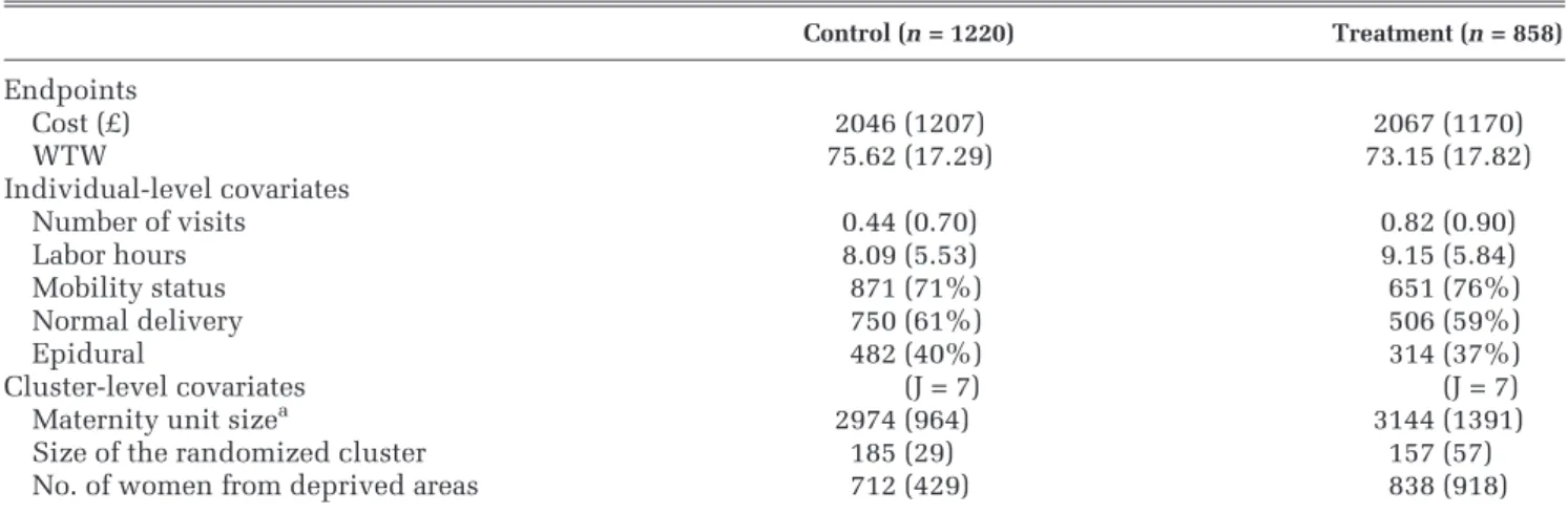
Table 1 Descriptive Statistics for the Fully Observed Data in the Case Study
Control (n= 1220) Treatment (n= 858) Endpoints Cost (£) 2046 (1207) 2067 (1170) WTW 75.62 (17.29) 73.15 (17.82) Individual-level covariates Number of visits 0.44 (0.70) 0.82 (0.90) Labor hours 8.09 (5.53) 9.15 (5.84) Mobility status 871 (71%) 651 (76%) Normal delivery 750 (61%) 506 (59%) Epidural 482 (40%) 314 (37%) Cluster-level covariates (J = 7) (J = 7)
Maternity unit sizea 2974 (964) 3144 (1391)
Size of the randomized cluster 185 (29) 157 (57)
No. of women from deprived areas 712 (429) 838 (918)
Note: Values are mean (standard deviation) for continuous variables andn(%) for binary variables. J = number of clusters. The willingness-to-wait (WTW) is a measure of process utility.
a. Total annual births.
Table 2 Correlation of Each Covariate with Cost and WTW Endpoints by Treatment Arm, and Standardized Mean Difference of Each Covariate between Treatment Groups
Control Group (n= 1220) Treatment Group (n= 858)
Cost WTW Cost WTW Standardized Differences
Number of visits 0.01 –0.10 0.09 –0.12 27% Labor hours 0.27 –0.67 0.30 –0.69 19% Mobility status 0.18 –0.59 0.18 –0.57 10% Normal delivery 0.30 –0.88 0.35 –0.89 5% Epidural 0.25 –0.66 0.27 –0.64 6% (J = 7) (J = 7) (J = 7) (J = 7)
Maternity unit sizea 0.30 –0.16 0.11 –0.59 14%
Size of the randomized cluster 0.55 0.27 –0.27 –0.91 86%
No. of women from deprived areas 0.16 0.64 0.19 –0.60 6%
Note: J = number of clusters; WTW = willingness to wait. a. Total annual births.
handling missing data may differ according to the proportion of individuals with missing data11,15 and the type of variables that predict missingness (e.g., continuous or binary, individual-level or clus-ter-level).30We have also allowed for different miss-ing data mechanisms, MCAR, MAR, and MNAR.22 In particular, allowing the data to be MNAR was motivated by the general concern in CEA that prob-ability of cost and outcome data may be conditional on the level of the endpoints.8,10,31For example, in our case study it may be expected that women with lower WTW may be more likely to have miss-ing WTW. Since the process utility endpoint, WTW, had lower ICC than the cost endpoint, we also hypothesized that there could be smaller differ-ences between methods for handling the missing WTW data than for handling missing costs.15,17
We started by considering missing costs only and assuming that the proportion of observations with missing data was 30%, a level typically seen in tri-al-based CEAs.8,10 In the first scenario (S0), we assumed that the missingness mechanism is MCAR, that is, the missingness is independent of any observed or unobserved variable. Then, we allowed costs to be MAR conditional on a continuous ual-level covariate, labor hours (S1); a binary individ-ual-level covariate, delivery mode (S2); a continuous cluster-level covariate, size of the randomized cluster (S3); and then all 3 covariates (S4). For these scenar-ios, we followed previous simulation studies32,33and
set the values forh1,h2, andh3such that there was a moderate level of association between each covari-ate and missingness (Pearson correlation coefficienty around 0.4). This assumed level of association, for example, between a binary covariate (e.g., delivery mode) and the missing costs (scenario S2), corre-sponded to an odds ratio of 0.21; that is, those women who had a normal (vaginal) delivery were about 5 times less likely to have unobserved cost data than those who did not. In the sensitivity analyses, we allowed small (correlation = 0.2) and high (correla-tion = 0.7) levels of associa(correla-tion. To achieve the desired percentage of missingness (30%) across the alternative scenarios, we chose h0 empirically,23 given the values assumed for h1, h2, and h3. We repeated scenarios S0 to S4 with the same parameter values but assuming that just the WTW was missing. We then assumed that information for both endpoints could be missing; the proportion of individuals miss-ing both endpoints is reported in Table 3 (last
col-umn). We assumed the same predictors of
missingness across both endpoints and treatment arms.
We then conducted sensitivity analyses (scenarios S5–S10) that considered further circumstances faced
Table 3 Description of the Alternative Scenarios
Scenario
Missingness Mechanism
Predictors of Missing Cost and WTW Endpointsa
% with Missing Data When Costs or WTW Is Set to Missing
% with Missing Data When Both Costs and WTW Are Set to Missing Individual Level Cluster Level Endpoints
Continuous Binary Continuous
S0 MCAR 3 3 3 3 30% 50% S1 MAR U 3 3 3 30% 48% S2 MAR 3 U 3 3 30% 50% S3 MAR 3 3 U 3 30% 49% S4 MAR U U U 3 30% 48% S5 MAR U U U 3 10% 16% S6 MAR U U U 3 50% 69%
S7 MAR 3 WTW only Costs only 3 30% 52%
S8 MAR Treatment only Control only 3 3 30% 49%
S9 MAR 3 3 U 3 Not applicableb 29%
S10 MNAR U U U U 30% 51%
Note: MAR = missing at random; MCAR = missing completely at random; WTW = willingness to wait.
a. Unless stated otherwise, each scenario assumed the same missingness predictors, and the same level of association between predictors and missingness, for both endpoints and treatment groups.
b. In this scenario, all cost and WTW data from 2 clusters were set to missing conditional on a cluster-level covariate, the proportion of women from deprived areas.
yFor example, the usual Pearson correlation coefficient between
a continuous covariate (X) and the binary missingness indicator (R) was calculated ascorrelation5covðR;XÞ=srsx, wheresris the stan-dard deviation ofR.
by CEAs that use CRTs where the relative perfor-mance of the methods may be anticipated to differ. We considered low (S5) and high (S6) proportions of missing data and different missingness predictors by endpoint (S7) and by treatment arm (S8), and we set 2 whole clusters to have unobserved endpoints conditional on a continuous cluster-level covariate (S9). In the final scenario (S10), we allowed for the data to be MNAR by setting the probability of costs and WTW being missing to be dependent on the level of the endpoints as follows:
Logit P Rc ij51jCij;Xij;Wij;Zj 5 hc01hc1Xij1hc2Wij1hc3Zj1dcCij Logit P Re ij51jEij;Xij;Wij;Zj 5 he01he1Xij1he2Wij1he3Zj1deEij
wheredcanddewere chosen to allow for different lev-els of association between the fully observed end-points and the probability of missingness. For the base case, we setdcanddeso that the level of associ-ation was moderate (correlassoci-ation = 0.4), which meant, for example, that women were 5% less likely to have missing WTW data (odds ratio = 0.95) for each unit increase in their WTW. We then considered alterna-tive levels of association between the endpoints and the probability of missingness (levels of correlation ranging from 0 to 0.7).
Implementation. For the imputation model, we
followed general recommendations and took an inclusive approach to variable selection by includ-ing all covariates associated with either endpoint in either treatment group.23,25,34 In each scenario, we included all 5 individual-level covariates: deliv-ery mode, number of previous hospital visits, mobil-ity status, type of pain relief, and labor hours; and all 3 cluster-level covariates: size of the randomized cluster, size of the maternity unit, and proportion of women from deprived areas. Hence, the imputation model included covariates beyond those used to sim-ulate the missing data. We specified joint models for the cost and WTW endpoints, separately for each treatment arm, and costs were log-transformed prior to imputation. We used the R packages ‘‘mice’’35and ‘‘pan’’19for the single-level and multilevel MI, respec-tively. We followed methodological guidance12,23and imputedM= 10 data sets in each scenario but allowed M= 50 in the sensitivity analyses.
For each missing data approach, we estimated incremental cost and WTW with a BVN multilevel
model (MLM) that assumed constant variances across clusters,5and we calculated the INB from the resul-tant parameter estimates. We assumed that there were no systematic imbalances in the baseline covari-ates, and we estimated linear additive treatment effects for both costs and WTW. For both MI methods, estimates were obtained by applying the MLM to each Mimputed data set. TheseM= 10 estimates were then combined by Rubin’s rules22to obtain MI estimates and standard errors.
In each scenario, we reported the mean (standard error) estimates for each method compared with the corresponding estimates from the fully observed data, defined as the ‘‘true’’ estimates. We reported the relative performance of each method as the per-centage differences in the mean estimates versus the true estimates. For example, the percentage mean dif-ferences (d) in the INB were calculated as
dðINBÞ5 jINBINBTTINBdj3100, where INBT is the true INB and INBd the INB estimated by a particular method. We also reported CEACs for S4. All analyses were implemented in R.
RESULTS
Missing Costs or WTW
In Table 4 (third column) we report means and standard errors of the incremental cost across scenar-ios in which 30% of women had missing costs. When costs were MCAR, all methods provided incremental costs similar to the true estimates obtained from the fully observed data. Under MAR, CCA gave point esti-mates that differed from the true incremental cost. In this setting with only the cost endpoint missing, the imputation approaches used information from the fully observed WTW endpoint, which was highly cor-related with the costs (r=20.4) as well as the base-line covariates to impute the costs. Across all scenarios, the multilevel MI provided estimates that were notably closer to the true estimates than the sin-gle-level MI. As the sinsin-gle-level MI did not recognize any dependency between observations within the cluster not explained by the cluster-level covariates, this approach also reported standard errors smaller than the true standard errors.
Table 4 (last column) also presents the results for the same scenarios but assuming that only WTW was missing (30%). Between-method differences were similar to those for missing costs; multilevel MI provided WTW estimates consistently closer to
the true estimates. However, for the WTW endpoint, a relatively low proportion of the variation was at the cluster level (ICC = 0.03), and so the single-level MI gave estimates that were somewhat closer to the true estimates than for the previous scenarios with missing costs. For some scenarios, CCA reported standard errors that differed from the true standard errors. This was because the subsamples with observed data happened to have more or less variabil-ity in their WTW or cost data than those observations whose endpoints were set to missing.
Missing Costs and WTW
In Table 5 we report incremental cost, incremental WTW, and INB assuming that for 30% of women
either costs or WTW was MAR; the proportion of
women with missing data for either endpoint was around 50% (Table 3) and for both endpoints was 10%. CCA and single-level MI provided point esti-mates of the INB that diverged from the true INB, and single-level MI also provided smaller standard errors. The divergence between the true and esti-mated INBs reflected those for the incremental costs and WTW, which were generally higher than for the previous scenarios where only one endpoint was set to missing (Table 4). Here, a higher proportion of women were missing either endpoint (approximately
50% v. 30%), and for those women missing both end-points the imputation was solely reliant on the cova-riate information. The multilevel MI gave point estimates and standard errors consistently close to the true INB.
The results were similar when we assumed low (correlation = 0.2) or high (correlation = 0.7) levels of association between the covariates and the proba-bility of missingness, when the number of imputa-tions was increased to 50.
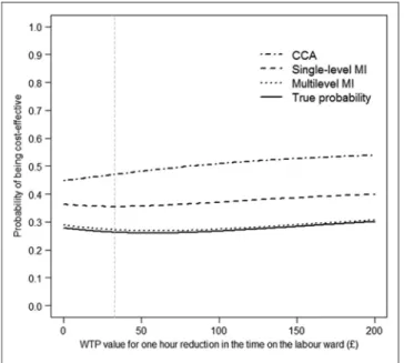
The CEACs illustrated for scenario S4 (Figure 1) showed that multilevel MI provided estimates closest to the true probability that the intervention is cost-effective across a wide range of WTP thresholds considered.
Sensitivity Analyses
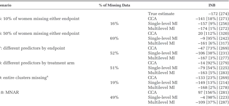
Both CCA and single-level MI provided divergent point estimates from the true estimates, even in cir-cumstances where each endpoint was missing for only 10% of women (84% complete cases) (Table 6). These estimates were further from the true esti-mates when 50% of observations were missing either endpoint (31% complete cases). By contrast, multi-level MI reported estimates closer to those from the fully observed data. Similar between-method differ-ences were reported when we allowed for different
Table 4 Incremental Cost with 30% Missing Costs, and Incremental WTW with 30% Missing WTW, for CCA, Single-Level MI, and Multilevel MI
Scenario Incremental Cost Incremental WTW
True estimates 160 (272) –0.45 (2.08)
S0: MCAR CCA 157 [2%] (284) –0.47 [4%] (2.10)
Single-level MI 159 [1%] (272) –0.44 [2%] (2.10) Multilevel MI 159 [1%] (272) –0.45 [0%] (2.11) S1: MAR conditional on an individual-level continuous variable CCA 123 [24%] (277) –0.32 [29%] (1.99)
Single-level MI 134 [16%] (228) –0.42 [7%] (2.10) Multilevel MI 160 [0%] (291) –0.44 [1%] (2.09) S2: MAR conditional on an individual-level binary variable CCA 116 [28%] (269) –0.28 [33%] (2.32)
Single-level MI 137 [14%] (223) –0.41 [9%] (2.13) Multilevel MI 154 [3%] (295) –0.45 [0%] (2.09) S3: MAR conditional on a cluster-level continuous variable CCA 131 [18%] (269) –0.31 [31%] (1.89)
Single-level MI 140 [13%] (224) –0.40 [11%] (2.12) Multilevel MI 161 [1%] (287) –0.44 [1%] (2.11)
S4: MAR conditional on all variables above CCA 125 [22%] (242) –0.34 [24%] (2.30)
Single-level MI 138 [14%] (207) –0.41 [9%] (1.66) Multilevel MI 162 [1%] (280) –0.45 [0%] (2.11) Note: Values are mean [% mean difference from the true estimate] (standard error). Scenarios S0–S4 were first generated by setting only costs to missing, and methods were compared to provide incremental cost (third column). These scenarios were then replicated by setting only missing WTW to missing, and methods were contrasted on the incremental WTW (last column). CCA = complete case analysis; MAR = missing at random; MCAR = missing com-pletely at random; MI = multiple imputation; WTW = willingness to wait.
predictors by endpoint (S7) and by randomized arm (S8) and when the costs and WTW of all the patients from 2 clusters were set to missing (S9).
Figure 2 illustrates the relative performance of each method under MNAR scenarios with increasing levels of association between the fully observed end-points and the probability of missingness. Here, mul-tilevel MI provides INB estimates that were relatively
close to the true INB when the correlation between the value of the endpoint and its missingness was fairly weak (correlation 0.2). Once we assumed a stronger relationship between the endpoints and the probability of missingness (correlation 0.4), none of the methods gave accurate estimates, but those from the multilevel MI were still closest to the true estimates.
DISCUSSION
This paper presents a multilevel MI approach for handling missing data in CEAs that use hierarchical data. This method is grounded on methodological guidance in the biostatistics literature which recom-mends its use for the analysis of missing data in hier-archical settings.12,16,19,23 In the context of a CEA alongside a CRT, we find that multilevel MI gives point estimates of cost-effectiveness and standard errors consistently close to those from the fully observed data. We therefore recommend that future studies adopt this approach for handling missing data in CEAs that use cluster trials, irrespective of the prevalence of missing data. CCA provides point estimates that are divergent from those of the fully observed data across all scenarios, and its use is dis-couraged. The estimates from the single-level MI are closer to the true estimates in less challenging set-tings, such as when the ICC is low and only one end-point has missing data. However, in most scenarios this MI approach leads to misleading point estimates
Table 5 Incremental Cost, Incremental WTW, and INB According to Method, across Different Scenarios with Costs and WTW Missing
Scenario % of Missing Data Incremental Cost Incremental WTW INBa
True estimates 160 (272) –0.45 (2.08) –172 (274) S1 48% CCA 73 [54%] (284) –0.27 [40%] (2.24) –82 [52%] (299) Single-level MI 118 [26%] (226) –0.34 [27%] (2.07) –129 [25%] (235) Multilevel MI 157 [2%] (294) –0.43 [4%] (2.11) –171 [1%] (295) S2 50% CCA 88 [45%] (254) –0.02 [95%] (2.17) –89 [55%] (253) Single-level MI 115 [28%] (217) –0.35 [22%] (2.11) –126 [27%] (223) Multilevel MI 158 [1%] (280) –0.46 [2%] (2.11) –173 [1%] (284) S3 49% CCA 59 [63%] (252) 0.35 [155%] (2.09) –48 [72%] (252) Single-level MI 105 [34%] (220) –0.30 [33%] (2.11) –115 [33%] (231) Multilevel MI 156 [3%] (285) –0.43 [4%] (2.14) –169 [2%] (292) S4 48% CCA 36 [80%] (272) 0.44 [198%] (2.23) –22 [87%] (282) Single-level MI 85 [47%] (214) –0.23 [49%] (2.17) –92 [47%] (220) Multilevel MI 153 [4%] (275) –0.46 [2%] (2.13) –167 [3%] (276)
Note: Values are mean [% mean difference from the true estimate] (standard error). CCA = complete case analysis; INB = incremental net benefit; MI = mul-tiple imputation; WTW = willingness-to-wait.
a. INB is valued at a WTP value of £32 for 1 hour reduction in the time on the labor ward.
Figure 1 Cost-effectiveness acceptability curves according to method, using estimates from scenario S4. CCA = complete case analysis; MI = multiple imputation; WTP = willingness to pay.
and standard errors. These scenarios include those when the cost endpoint, which had a higher ICC, is missing and when a higher proportion of patients are missing either endpoint.
Single-level MI does not recognize that observa-tions within each cluster may be correlated, and it
assumes that there is more information than there actually is and, hence, that the resultant precision of the resultant estimates is overstated. Our results suggest that approaches that ignore the clustering not only exaggerate the precision but can also lead to inappropriate point estimates. The way that sin-gle-level MI weights individuals within each cluster differs from that of multilevel MI. The resultant point estimates can differ between single-level and multi-level MI approaches when the randomized clusters are of different size and the relationship between cluster size and either endpoint differs by treatment arm. Previous work has shown that in such circum-stances, multilevel versus single-level analysis mod-els can give different point estimates.6,36A previous simulation study for handling missing univariate endpoint data in CRTs also found that single-level MI underestimates the uncertainty around the estimates.15
A previous paper proposed multilevel MI for CEAs that use cluster trials in a reanalysis of a single case study.20We extend this work by assessing the
meth-ods’ performance against estimates obtained from fully observed cases. This allowed the methods to be compared across a wide range of circumstances typically encountered in CEAs that use CRTs.18 We found that unless data are MCAR, which is unlikely,
Table 6 INB (WTP value: £32 per hour) for Each Method across Sensitivity Analysis Scenarios Scenario % of Missing Data INB
True estimate –172 (274)
S5: 10% of women missing either endpoint CCA –141 [18%] (271)
16% Single-level MI –157 [9%] (256)
Multilevel MI –174 [1%] (272)
S6: 50% of women missing either endpoint CCA 20 [112%] (320)
69% Single-level MI –9 [95%] (242)
Multilevel MI –161 [6%] (317)
S7: different predictors by endpoint CCA –47 [73%] (269)
52% Single-level MI –106 [38%] (231)
Multilevel MI –167 [3%] (277)
S8: different predictors by treatment arm CCA –14 [92%] (279)
51% Single-level MI –79 [54%] (225)
Multilevel MI –163 [5%] (283)
S9: entire clusters missinga CCA –133 [23%] (269)
19% Single-level MI –149 [13%] (214)
Multilevel MI –168 [2%] (278)
S10: MNAR CCA 97 [156%] (281)
49% Single-level MI –4 [98%] (223)
Multilevel MI –109 [37%] (287)
Note: Values are mean [% mean difference from the true estimate] (standard error). CCA = complete case analysis; INB = incremental net monetary benefit; MI = multiple imputation; MNAR = missing not at random; WTP = willingness to pay.
a. All cost and WTW data from 2 clusters were set to missing conditional on a cluster-level covariate, the number of women from deprived areas; The bench-mark is scenario S4.
Figure 2 INB (WTP value: £32 per hour) according to method for MNAR scenarios (the benchmark is S4) at increasing levels of asso-ciation between endpoints and missingness. CCA = complete case analysis; INB = incremental net monetary benefit; MI = multiple imputation; MNAR = missing not at random; WTP = willingness to pay.
CCA and the single-level MI approach appear inap-propriate for studies with clustered data. The multi-level MI approach is compatible with MLMs for handling cost-effectiveness data with a multilevel structure.2,3,5 Previous simulations studies5,36 showed that MLMs developed for CEAs that use CRTs performed relatively well even with a small number of clusters (3 per arm). In our case study, which had 7 clusters per arm, the use of multilevel MI for handling the missing data combined with MLMs for the analysis provided both point estimates and uncertainty measures close to the true values.
Previous papers have proposed single-level MI approaches for handling missing data in CEAs.7–11 Simulations have shown that single-level MI can per-form relatively well with a single endpoint and when the data are not hierarchical.10,11 More generally,
CEAs based on patient-level data tend to use hierar-chical designs such as multicenter and cluster trials, where the data can be anticipated to have a multilevel structure. The multilevel MI approach proposed, although illustrated in the context of a CEA from a CRT, can be extended to other hierarchical settings such as multicenter or multinational studies.
While multilevel MI has been proposed more generally for handling missing data that have a hierar-chical structure,12,16,19the CEA context brings addi-tional challenges for the method. In this setting, methods need to recognize that the probability that one endpoint is missing may be dependent on the other endpoint; for example, patients in worse health may be less likely to return resource use question-naires. Here, we recognized this by considering joint imputation models for missing costs and WTW (Mod-els 1 and 2 above), which used the information of the observed endpoint to impute the missing endpoint. In addition, we acknowledged that costs tend to have a right-skewed distribution by log-transforming them before any imputation and back-transforming the data after imputation.8,11 As data were back-transformed before the analytical models were applied, this avoided the retransformation problem that can occur when one is back-transforming esti-mates from log-normal endpoint models.37 For the
analytical model, we considered bivariate normal MLMs, which have been shown to perform well across different circumstances in CEAs that use CRTs, including when costs are skewed.5,6,36
Our analysis compared a multilevel MI approach that used a joint normal distribution with a commonly used single-level MI procedure that uses a full conditional specification (sometimes called the
chained equations approach).35 When instead we
implemented both single-level MI and multilevel MI using the chained equations approach, differen-ces in the estimates between the single-level and mul-tilevel approach remained the same. The mulmul-tilevel MI approach can be readily implemented in available software; we chose to use the R package and to append code to help disseminate the method (Appendix 2), but other available software options include the mi macro in MLwiN12 and the REAL-COM-impute macros.38
MI methods, like other principled approaches for handling missing data, such as maximum likelihood estimation and full-Bayesian analyses (estimated via MCMC), assume that the data are MAR. In practice, data may be missing dependent on unobserved fac-tors (e.g., patient lifestyle facfac-tors); that is, the data may be MNAR. This paper considered settings in which data were assumed to be MNAR, and it showed that cost-effectiveness results by either MI approach were sensitive to departures from the MAR. In this case study, multilevel MI reported cost-effectiveness estimates that were closest to the true estimates across the alternative MNAR scenarios. However, it is important for future CEAs to conduct structural sensitivity analyses to consider how to handle possi-ble MNAR mechanisms. MI approaches under MAR are amenable to such sensitivity analyses, and this is an ongoing area of methodological research.39
This paper has some limitations. First, we did not undertake a full simulation study, which would have allowed metrics such as bias, mean squared error, and confidence interval coverage to be compared across the methods. Previous simulation studies15,17 have suggested that multilevel MI outperforms single-level MI with clustered data, and either approach can reduce bias versus CCA. Here, we chose a design that allowed us to compare the different methods across a range of plausible mechanisms, which gave rise to incomplete data in a typical CEA alongside a CRT. By taking this approach, we could examine the implications of the choice of method on cost-effectiveness estimates for alternative missing data mechanisms. These findings will help inform a future simulation study. Second, the paper has taken data from a single case study and investigated missing data for costs and a measure of process utility. More generally, the missing data may take different forms to those considered here; for example, the endpoint may be binary or time to event, and the pattern of the missing data may be more complex (e.g., different components of resource use). Third, our analyses were based on a single replication of the missing data, but when we conducted 1000 replications for
particular scenarios, the findings were unchanged. Fourth, this study contrasted multilevel MI with sin-gle-level MI, which has been previously proposed for CEAs, and CCA, an approach commonly taken in applied studies. However, other methods for han-dling missing data in CEAs, such as inverse probabil-ity weighting23 and full-Bayesian approaches,40 could also be extended to allow for clustering.
The findings from this paper provoke several areas for further research. Future studies could consider the relative performance of a broader range of meth-ods in more general circumstances faced by CEAs. In particular, it would be useful to contrast full-Bayesian approaches with multilevel MI for handling other complex structures, for example, CEAs that have longitudinal data. Here, it would be interesting to contrast the potential flexibility that Bayesian approaches may afford with respect to exploiting external data, with the additional requirements of specifying prior distributions. Second, further work is needed to develop approaches for exploring the sensitivity the cost-effectiveness results to depar-tures from the MAR assumption, by considering a range of possible MNAR mechanisms.23,39,41Such approaches can allow analysts to present decision makers with a fuller representation of the uncertainty that surrounds the CEA results, to facilitate a sounder basis for future decisions.
ACKNOWLEDGMENTS
The authors are grateful to Graham Scotland and Paul McNamee, for providing access to the Maternity data set, and to Simon Thompson, James Carpenter, Simon Dixon, Zia Sadique, and John Cairns for their helpful comments.
REFERENCES
1. Willan A, Briggs A. Statistical Analysis of Cost-effectiveness Data. Chichester, UK: John Wiley & Sons; 2006.
2. Grieve R, Nixon R, Thompson SG, Cairns J. Multilevel models for estimating incremental net benefits in multinational studies. Health Econ. 2007;16(8):815–26.
3. Manca A, Lambert PC, Sculpher M, Rice N. Cost-effectiveness analysis using data from multinational trials: the use of bivariate hierarchical modeling. Med Decis Making. 2007;27(4):471–90. 4. Nixon RM, Thompson SG. Methods for incorporating covariate adjustment, subgroup analysis and between-centre differences into cost-effectiveness evaluations. Health Econ. 2005;14(12):1217–29. 5. Gomes M, Ng ESW, Grieve R, Nixon R, Carpenter J, Thompson SG. Developing appropriate methods for cost-effectiveness analy-sis of cluster randomized trials. Med Decis Making. 2012;32(2): 350–61.
6. Grieve R, Nixon R, Thompson SG. Bayesian hierarchical models for cost-effectiveness analyses that use data from cluster random-ized trials. Med Decis Making. 2010;30(2):163–75.
7. Blough DK, Ramsey S, Sullivan SD, Yusen R. The impact of using different imputation methods for missing HRQoL in cost-ef-fectiveness analysis of lung-volume-reduction surgery. Health Econ. 2009;18(1):91–101.
8. Briggs A, Clark T, Wolstenholme J, Clarke P. Missing . . . pre-sumed at random: cost-analysis of incomplete data. Health Econ. 2003;12(5):377–92.
9. Grieve R, Cairns J, Thompson SG. Improving costing methods in multicentre economic evaluation: the use of multiple imputation for unit costs. Health Econ. 2010;19(8):939–54.
10. Oostenbrink JB, Al MJ. The analysis of incomplete cost data due to dropout. Health Econ. 2005;14(8):763–76.
11. Yu LM, Burton A, Rivero-Arias O. Evaluation of software for multiple imputation of semi-continuous data. Stat Methods Med Res. 2007;16(3):243–58.
12. Carpenter J, Goldstein A. Multiple imputation using MLwiN. Multilevel Modelling Newsletter. 2004;16(2):9–18.
13. Noble SM, Hollingworth W, Tilling K. Missing data in trial-based cost-effectiveness analysis: the current state of play. Health Econ. 2012;21(2):187–200.
14. Little RJ, Rubin DB. Statistical Analysis with Missing Data. New York: Wiley; 2002.
15. Andridge RR. Quantifying the impact of fixed effects modeling of clusters in multiple imputation for cluster randomized trials. Biometrical J. 2011;53(1):57–74.
16. Goldstein H, Carpenter J, Kenward MG, Levin KA. Multilevel models with multivariate mixed response types. Stat Model. 2009;9(3):173–97.
17. Taljaard M, Donner A, Klar N. Imputation strategies for miss-ing continuous outcomes in cluster randomized trials. Biometrical J. 2008;50(3):329–45.
18. Gomes M, Grieve R, Nixon R, Edmunds WJ. Statistical methods for cost-effectiveness analyses that use data from cluster random-ized trials: a systematic review and checklist for critical appraisal. Med Decis Making. 2012;32(1):209–20.
19. Schafer JL, Yucel RM. Computational strategies for multivari-ate linear mixed-effects models with missing values. J Comput Graph Stat. 2002;11(2):437–57.
20. Diaz-Ordaz K, Kenward MG, Grieve R. Handling missing val-ues in cost-effectiveness analyses that use data from cluster rando-mised trials. J R Stat Soc Series A. Forthcoming.
21. Scotland G. Elicitation and application of preference values in economic evaluation: case studies in reproductive health. PhD the-sis, Health Economics Research Unit, University of Aberdeen; 2012. 22. Rubin DB. Multiple Imputation for Nonresponse in Surveys. New York: Wiley; 1987.
23. Carpenter J, Kenward MG. Multiple Imputation and its Appli-cation. Chichester, UK: Wiley; 2013.
24. Schafer AL. Multiple imputation with PAN. In: Collins L, Sayer A, eds. New Methods for the Analysis of Change. Washing-ton, DC: American Psychological Association; 2001:357-377. 25. White IR, Royston P, Wood AM. Multiple imputation using chained equations: issues and guidance for practice. Stat Med. 2011;30(4):377–99.
26. Cheyne H, Hundley V, Dowding D, et al. Effects of algorithm for diagnosis of active labour: cluster randomised trial. BMJ. 2008;337:a2396.
27. Kenward MG, Roger JH. Small sample inference for fixed effects from restricted maximum likelihood. Biometrics. 1997; 53(3):983–97.
28. Scotland GS, McNamee P, Cheyne H, Hundley V, Barnett C. Women’s preferences for aspects of labor management: results from a discrete choice experiment. Birth. 2011;38(1):36–46. 29. Taylor S, Armour C. Consumer preference for dinoprostone vaginal gel using stated preference discrete choice modelling. PharmacoEconomics. 2003;21(10):721–35.
30. Black AC, Harel O, McCoach DB. Missing data techniques for multilevel data: implications of model misspecification. J Appl Stat. 2011;38(9):1845–65.
31. Fielding S, Fayers PM, McDonald A, McPherson G, Campbell MK, Group RS. Simple imputation methods were inadequate for missing not at random (MNAR) quality of life data. Health Qual Life Outcomes. 2008;6:57.
32. Kang JDY, Schafer JL. Demystifying double robustness: a com-parison of alternative strategies for estimating a population mean from incomplete data. Stat Sci. 2007;22(4):523–39.
33. Zhang M, Tsiatis AA, Davidian M. Improving efficiency of inferences in randomized clinical trials using auxiliary covariates. Biometrics. 2008;64(3):707–15.
34. Sterne JA, White IR, Carlin JB, et al. Multiple imputation for missing data in epidemiological and clinical research: potential and pitfalls. BMJ. 2009;338:b2393.
35. van Buuren S, Groothuis-Oudshoorn K. mice: Multivariate Imputation by Chained Equations in R. J Stat Softw. 2011;45(3): 1–67.
36. Gomes M, Grieve R, Nixon R, Ng ES, Carpenter J, Thompson SG. Methods for covariate adjustment in cost-effectiveness analy-sis that use cluster randomised trials. Health Econ. 2012;21(9): 1101–18.
37. Manning WG, Mullahy J. Estimating log models: to transform or not to transform? J Health Econ. 2001;20(4):461–94.
38. Carpenter JR, Goldstein H, Kenward MG. REALCOM-IMPUTE software for multilevel multiple imputation with mixed response types. J Stat Softw. 2011;45(5):1–14.
39. Carpenter JR, Kenward MG, White IR. Sensitivity analysis after multiple imputation under missing at random: a weighting approach. Stat Methods Med Res. 2007;16(3):259–75.
40. Lambert PC, Billingham LJ, Cooper NJ, et al. Estimating the cost-effectiveness of an intervention in a clinical trial when partial cost information is available: a Bayesian approach. Health Econ. 2008;17(1):67–81.
41. Mason A, Richardson S, Plewis I, Best N. Strategy for model-ling nonrandom missing data mechanisms in observational studies using Bayesian methods. J Off Stat. 2012;28(2):279–302.