A Mixed Integer Quadratic Programming Model for the Low Autocorrelation Binary Sequence Problem

A MIXED INTEGER QUADRATIC PROGRAMMING MODEL FOR THE LOW AUTOCORRELATION BINARY

SEQUENCE PROBLEM∗

Jozef Kratica

Abstract. In this paper the low autocorrelation binary sequence problem (LABSP) is modeled as a mixed integer quadratic programming (MIQP) problem and proof of the model’s validity is given. Since the MIQP model is semidefinite, general optimization solvers can be used, and converge in a finite number of iterations. The experimental results show that IQP solvers, based on this MIQP formulation, are capable of optimally solv-ing general/skew-symmetric LABSP instances of up to 30/51 elements in a moderate time.

1. Introduction. The low autocorrelation binary sequence problem (LABSP) is a very hard combinatorial optimization problem with a quite simple formulation. The mathematical formulation of LABSP is based on a binary

ACM Computing Classification System(1998): G.1.6, I.2.8.

Key words: Integer programming, Quadratic programming, low autocorrelation binary se-quence problem.

∗_{This research was partially supported by the Serbian Ministry of Education and Science} under projects 174010 and 174033.

sequencesof the lengthn. Lets∈ {−1,1}n, i.e.,sis represented by (s1,s2, . . . , sn), where si ∈ {−1,1} for 1 ≤ i ≤n. Each sequence s is associated with the

value of its energy function, which is defined as follows:

(1) E(s) = n−1 X k=1 C_k2(s), where Ck(s) = n−k X i=1 sisi+k

Then, the low autocorrelation problem for binary sequences with length n, can be formulated as finding a sequencesof the lengthnwhose energy function is as low as possible. The second measure of the quality of the sequence sis a merit factor

(2) F(s) = n

2 2E(s),

defined by Bernasconi in [2]. Mathematically, LABSP can be formulated as max

s∈{−1,1}nF(s). Both formulations are equivalent, and either of them can be used

when it is convenient.

As can be seen from (1), the objective function has degree four and de-cision variables are integer. Therefore, the existing LABSP formulation cannot be solved by any existing general optimization programming package, since they are able to solve:

• global optimization models, where decision variables have real values;

• integer linear programming models;

• semidefinite quadratic programming models.

In order to enable the use of existing state-of-the-art integer optimization packages for solving LABSP, it is reformulated as a semidefinite mixed integer quadratic programming problem in Section 3, together with the proof of the equivalence of the two models.

One subset of the low autocorrelation binary sequences that has gained much attention in the search of LABSP are so-called skew-symmetric sequences. They are sequences with the odd length n, fulfilling the condition (3):

where m = n+ 1

2 . Since for the sequences with the odd values of k, Ck(s) = 0 and because the search space is 2m−1

times smaller, the running time of the methods dealing only with the skew-symmetric sequences is several times shorter, compared to the general case. Although the asymptotic value of F(s) obtained for these sequences is the same as for the general case, the true global optimum is not skew-symmetric for many values ofn (for LABSP withn= 19,23,25, . . ., the global optima are not skew-symmetric).

The rest of the paper is organized as follows. In Section 2, previous work on LABSP is presented. A new mixed integer quadratic programming (MIQP) model is given in Section 3, together with proof of its correctness. Section 4 contains computational results of two state-of-the-art integer linear and quadratic solvers based on the proposed MIQP formulation. Section 5 contains conclusions and directions to future work.

2. Previous work. LABSP has been deeply studied since the 1960s by the communities of both physics and artificial intelligence. There are two reasons behind this interest:

• It arises in many diverse areas, including statistical mechanics and config-uration state analysis [2], calibration of surface profile metrology tools [1], satellite and space applications [9], digital signal processing [19], etc.;

• LABSP is also a significant challenge to exact and/or heuristic applications, since it is known that the problem has “bit-flip” neighborhood structure of combinatorial landscapes [6, 7]. With this type of neighborhood, it is extremely steep around the optimum, which is sometimes referred to as “golf hole” landscapes, and it poses a very difficult optimization problem. In this case, small changes in argument values usually cause a drastic difference in objective value. For example, alteration of only one bit in the binary sequencescan affect an objective value change by several tens of percents. For these reasons LABSP is also listed in the CSPLIB library as problem 005.

Although Golay in [10] estimated that lim

n→∞F(s) = 12.32, it is not good

enough, because for the dimensions between 21 and 60 the merit factor varies from F(s) = 5.627 for n= 23 to F(s) = 9.85 for n= 27, which is obviously far from the estimated limit 12.32.

The state-of-the-art exact method given in [15, 16] is based on exhaustive search and it solves the problem optimally up to n = 60. The experimental research was carried out for several days on a multiprocessor cluster of 160 CPUs. It is the largest dimension with a known optimal solution.

A detailed description of all metaheuristic approaches for solving LABSP is out of this paper’s scope, so only several successful applications are mentioned:

• A hybrid evolutionary approach described in [3] combines the evolutionary search described in [17] and the Kerninghan-Lin heuristic defined in [13]. This evolutionary approach uses a specific termination criterion based on statistical analysis of known optimal solutions and their asymptotic behav-ior.

• In [5], the authors presents a constraint programming approach hybridized with local search algorithms incorporated into the tabu search program framework. The initial configuration is randomly generated, and in each iteration the best move in the neighborhood of the current solution is se-lected. The tabu component maintains a fixed length tabu list in order to avoid flipping a recently considered variable. It also uses an aspira-tion criterion to overwrite the tabu status when the move would lead to the best solution found so far. The restarting component of the approach simply re-initializes the search from a random configuration, whenever the best configuration found so far has not been improved upon the predefined number of iterations. Computational experiments show that the presented tabu search algorithm quickly finds solutions for the instances up ton= 32 (in a few seconds or less), and finds solutions in reasonable time for the re-maining instances. Moreover, it finds the optimal LABSP sequences for the values up ton= 48 and it is about 8 to 55 times faster than the previous local search approach presented in the literature.

• In [20], Greedy Randomized Adaptive Search Procedures (GRASP) are applied to tackle the LABSP problem. Using greedy solutions as starting points for local search will usually lead to suboptimal solutions, since a greedy starting solution is less likely to be in the basin of the attraction of a global optimum. To avoid producing the same solution in each iteration, a list of best candidates, called the restricted candidate list, is constructed according to their greedy function values. One of the best solutions but not necessarily the top candidate is selected randomly from that list. After

finding the local optima,n/10 random positions in the sequencesare flipped several times, in order to generate a new set of initial sequences for the next iteration. Afterward, a steepest descent local search procedure was applied, that moves the solution to the best sequence in the neighborhood until a local optimum is reached. In order to test the algorithm on larger instances, the method is also adapted to explore skew-symmetric solutions.

• A detailed analysis of different stand-alone local search strategies is given in [8]. This analysis is later used in embedding the best local search strategy within other metaheuristic approaches. The results indicate that the pure evolutionary algorithm cannot cope with the complexity of the problem and the assistance of the local-search operators is required to provide optimal or suboptimal results being consistent. As a best choice for solving LABSP, a memetic algorithm endowed with a tabu search local searcher is proposed, and that approach consistently finds optimal sequences in considerably less time than the approaches previously reported in the literature.

• Another metaheuristic method for solving LABSP, based on the stochastic local search (SLS), is presented in [12]. In-depth analysis of LABSP fitness landscape and the white-box visualization get insights on how SLS can be effective and lead to a slightly better strategy.

• A local search algorithm described in [18] uses a quite different strategy compared to previous local search approaches. It is based on the random-ized form of backtracking. In that way, the optimization problem is reduced to a series of constraint satisfaction problems which are solved iteratively, with decreasing upper bounds of the given objective function. Experimen-tal results indicate that the algorithm is time consuming. For example, the average running time forn= 40 is over 1000 seconds.

• An electromagnetism-like approach (EM) for solving the low autocorrela-tion binary sequence problem (LABSP) is applied in [14]. Movement based on the attraction-repulsion mechanisms combined with the proposed scaling technique directs the EM to the promising search regions. Fast implemen-tation of the local search procedure additionally improves the efficiency of the overall EM system.

3. A new MIQP formulation. As has been stated previously, the MIQP formulation presented in this section is the first attempt, to the author’s knowledge, to modify the LABSP mathematical formulation to be possibly solved by existing optimization packages. Moreover, when the problem is formulated as semidefinite MIQP, it is later possible to use the principles of semidefinite programming to possibly design an exact method for LABSP.

Since optimization packages allow better treatment for binary decision variables compared to integer decision variables, andsi∈ {−1,1}, it is convenient

to translate it to the binary decision variable xi∈ {0,1} by simple scaling

(4) si = 2·xi−1

or equivalently

(5) xi =

si+ 1

2

Let the other decision variables be defined as follows:

(6) yik=xi·xi+k

and

(7) zk=Ck(s)

Then, the mixed integer quadratic programming (MIQP) formulation is:

(8) min n−1 X k=1 z2 k s.t. (9) −zk+ 4· n−k X i=1 yik−2· n−k X i=1 xi−2 n−k X i=1 xi+k=k−n k= 1, . . . , n−1 (10) yik ≤ 1 2xi+ 1 2xi+k k= 1, . . . , n−1, i= 1, . . . n−k (11) yik≥xi+xi+k−1 k= 1, . . . , n−1, i= 1, . . . n−k

(12) xi, yik∈ {0,1}, zk∈[−n, n] k= 1, . . . , n−1, i= 1, . . . n−k

As it can be seen, there are nreal variables, n·(n+ 1)

2 binary variables andn2

−1 constraints. Now, we can define ObjM IQP(x, y, z) = n−1 X k=1 z2 k subject to (9)–(12).

Let us show that the solution of this MIQP formulation is the solution of the LABSP.

Lemma 1. Let s be a sequence from {−1,1}n. Then there exists a solution (x, y, z) of the system (9)–(12) such that ObjM IQP(x, y, z) is not more than E(s).

P r o o f. Let the decision variables (x, y, z) be defined as (5)–(7). We will prove that this vector satisfies the system (9)–(12) andObjM IQP(x, y, z)6E(s).

Constraints (12) are satisfied by definitions of the decision variables (5)–(7). If xi = xi+k = 1 then yik = xi·xi+k = 1 = 1 2xi + 1 2xi+k = 1 2 + 1 2. If xi = 0 or xi+k = 0 (or both are equal to 0) then yik = xi ·xi+k = 0, while

1 2xi+

1

2xi+k≥0, since decision variablesx are non-negative. Therefore, in both cases yik ≤

1 2xi+

1

2xi+k holds, implying that constraints (10) are satisfied. Similarly, if xi =xi+k = 1 then yik =xi·xi+k= 1 = xi+xi+k−1 = 1.

If xi = 0 or xi+k = 0 (or both are equal to 0) then yik = xi·xi+k = 0, while

xi+xi+k−1≤0, since decision variables x are at most one. Therefore, in both

cases yik ≥xi+xi+k−1 holds, implying that constraints (11) are satisfied.

Using the definitions of the decision variables given in (4)–(7) we have zk

=Ck(s) = n−k X i=1 si·si+k = n−k X i=1 (2·xi−1)·(2·xi+k−1)= = n−k X i=1 (4·xi·xi+k−2·xi−2·xi+k+ 1) = 4· n−k X i=1 xi·xi+k−2· n−k X i=1 xi −2· n−k X i=1 xi+k+ n−k X i=1 1 = 4· n−k X i=1 yik−2· n−k X i=1 xi−2· n−k X i=1 xi+k+n−k. Therefore,

zk= 4· n−k X i=1 yik−2· n−k X i=1 xi−2· n−k X i=1

xi+k+n−k, which is equal as constraint (9).

It can be seen that by (7)zk=Ck(s) holds. Then n−1 X k=1 z_k2 = n−1 X k=1 Ck(s)2=

E(s). We have one solution (x, y, z) with the objective function value equals to E(s), thereforeObjM IQP(x, y, z)6E(s).

Lemma 2. Let (x, y, z) be a solution to (9)–(12). Then there exists a sequences such that E(s) is not more than ObjM IQP(x, y, z, u).

P r o o f. The first step is to prove that constraints (10) and (11) on binary decision variablesyik, xi and xk are equivalent as yik =xi·xi+k. Actually, (10)

implies that ifyik= 1 then because of the binary nature of the decision variables

x,xi=xi+k= 1 must be satisfied. On the other hand, (11) implies that ifyik = 0

then xi+xi+k ≤ 1 so either one of them (or both xi and xi+k) must be equal

to zero. Similarly, in the other direction, when xi = xi+k = 1 by (11) must be

yik = 1, and whenxi = 0 orxi+k= 0, constraint (10) implies yik= 0.

Let the sequencesbe defined by (4). Then, as in the Proof of Lemma 1, Ck(s) = n−k X i=1 si·si+k = n−k X i=1 (2·xi−1)·(2·xi+k−1) = = n−k X i=1 (4·xi·xi+k−2·xi−2·xi+k+ 1) = 4· n−k X i=1 xi·xi+k−2· n−k X i=1 xi −2· n−k X i=1 xi+k+ n−k X i=1 1 = 4· n−k X i=1 yik−2· n−k X i=1 xi−2· n−k X i=1 xi+k+n−k. From constraint (9) it follows thatCk(s) =zk, so E(s) = n−1 X k=1 C2 k(s) = n−1 X k=1 z2 k =ObjM IQP(x, y, z).

Theorem 1. _{Sequence shas minimal energy E(s) if and only if there is} an optimal solution (x, y, z) of (8)–(12).

P r o o f. The direction (⇒) can be easily deduced from Lemma 1. The other direction (⇐) directly follows from Lemma 2.

Note that the objective function (8) is obviously semidefinite, since it is the sum of squares, so integer quadratic programming packages can be used, and they converge in a finite number of iterations.

It is obvious that for the skew-symmetric LABSP, for decision variables, the constraint (3) is stated as:

(13) xm+i=    xm−i, i is even 1−xm−i, i is odd

Therefore, the MIQP formulation for skew-symmetric LABSP is (8)-(13).

4. Experimental results. In order to illustrate the ability of the pre-sented MIQP model for LABSP, a number of experimental testings are provided. The MIQP model is tested on two state-of-the-art integer linear and quadratic programming solvers: CPLEX [4] version 12.1 and Gurobi [11] version 4.0. All computation experiments are executed on a single core of Quad Core 2.5 GHz PC computer with 4 GB RAM.

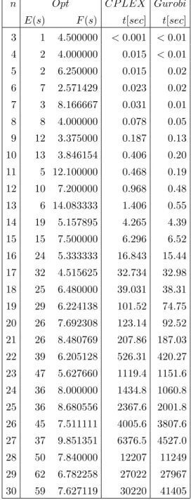
Table 1 presents the results of CPLEX and Gurobi solvers using the pro-posed MIQP model on LABSP instances with 3 ≤ n≤ 30. In the first column the dimensionnis given. The next two columns contain the optimal energy E(s) and merit factor F(s) for the given dimension. The last two columns contain total running times needed to obtain and verify the optimal solution of CPLEX and Gurobi solver, respectively.

Table 2 displays the results of CPLEX and Gurobi solvers using the pro-posed MIQP model on skew-symmetric LABSP instances with 3 ≤ n ≤ 51, presented in the same way as in Table 1.

As can be seen from Table 1, both solvers are able to obtain optimal solutions for general LABSP instances up ton= 30 in moderate time. Although the obtained results are encouraging, this approach is not capable of obtaining new and unknown optimal solutions for dimensions n >60.

However, for skew-symmetric LABSP instances optimal solutions are ob-tained for dimensions up to n = 51. For some of the instances, to the author’s knowledge, this is the first report of skew-symmetric optimal results in the liter-ature.

In order to obtain some insights for metaheuristic performance for solving LABSP, results of several such approaches, mentioned in Section 2, are presented

Table 1. CPLEX and Gurobi results on general LABSP instances

n Opt CP LEX Gurobi

E(s) F(s) t[sec] t[sec] 3 1 4.500000 <0.001 <0.01 4 2 4.000000 0.015 <0.01 5 2 6.250000 0.015 0.02 6 7 2.571429 0.023 0.02 7 3 8.166667 0.031 0.01 8 8 4.000000 0.078 0.05 9 12 3.375000 0.187 0.13 10 13 3.846154 0.406 0.20 11 5 12.100000 0.468 0.19 12 10 7.200000 0.968 0.48 13 6 14.083333 1.406 0.55 14 19 5.157895 4.265 4.39 15 15 7.500000 6.296 6.52 16 24 5.333333 16.843 15.44 17 32 4.515625 32.734 32.98 18 25 6.480000 39.031 38.31 19 29 6.224138 101.52 74.75 20 26 7.692308 123.14 92.52 21 26 8.480769 207.86 187.03 22 39 6.205128 526.31 420.27 23 47 5.627660 1119.4 1151.6 24 36 8.000000 1434.8 1060.8 25 36 8.680556 2367.6 2001.8 26 45 7.511111 4005.6 3807.6 27 37 9.851351 6376.5 4527.0 28 50 7.840000 12207 11249 29 62 6.782258 27022 27967 30 59 7.627119 30220 41405

Table 2. CPLEX and Gurobi results on skew-symmetric LABSP instances

n Opt CP LEX Gurobi

E(s) F(s) t[sec] t[sec] 3 1 4.500000 <0.001 <0.01 5 2 6.250000 <0.001 0.020 7 3 8.166667 0.015 <0.01 9 12 3.375 0.046 0.03 11 5 12.1 0.015 0.01 13 6 14.083333 0.015 0.06 15 15 7.5 0.421 0.19 17 32 4.515625 0.953 0.58 19 33 5.469697 1.500 0.83 21 26 8.480769 2.953 1.41 23 51 5.186275 7.343 4.36 25 52 6.009615 11.718 13.11 27 37 9.851351 19.437 22.30 29 62 6.782258 62.593 42.42 31 79 6.082278 86.765 98.72 33 88 6.1875 167.69 440.23 35 89 6.882022 369.63 298.39 37 106 6.457547 644.63 1037.0 39 99 7.681818 1099.0 1627.1 41 108 7.782407 2215.1 2080.5 43 109 8.481651 3411.3 4333.3 45 118 8.580508 5309.9 7900.1 47 135 8.181481 10810 14322 49 136 8.827206 22839 28111 51 153 8.5 42443 56709

in Tables 3-5. Note that direct comparison of exact and metaheuristic approaches are not fair, since the second approach is not able to verify the optimality of the solution, even if it has reached the optimal solution, which is not always the case. In that sense, the exact method is not only able to verify the optimality of the

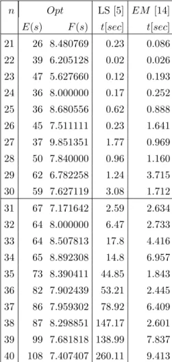
Table 3. Metaheuristic results on LABSP instances with 21≤n≤40 n Opt LS [5] EM [14] E(s) F(s) t[sec] t[sec] 21 26 8.480769 0.23 0.086 22 39 6.205128 0.02 0.026 23 47 5.627660 0.12 0.193 24 36 8.000000 0.17 0.252 25 36 8.680556 0.62 0.888 26 45 7.511111 0.23 1.641 27 37 9.851351 1.77 0.969 28 50 7.840000 0.96 1.160 29 62 6.782258 1.24 3.715 30 59 7.627119 3.08 1.712 31 67 7.171642 2.59 2.634 32 64 8.000000 6.47 2.733 33 64 8.507813 17.8 4.416 34 65 8.892308 14.8 6.957 35 73 8.390411 44.85 1.843 36 82 7.902439 53.21 2.445 37 86 7.959302 78.92 6.409 38 87 8.298851 147.17 2.601 39 99 7.681818 138.99 7.837 40 108 7.407407 260.11 9.413

solution, but much of its running time is used for verification of the solutions’s optimality, although it can be already reached. Additionally, a direct comparison can not be performed, since CPLEX and Gurobi are general quadratic integer programming solvers, and all mentioned metaheuristic methods are not general et all, but implemented and applied specially for LABSP.

Tables 3–5 display the results of metaheuristic approaches on LABSP instances with 21 ≤n ≤40, 41 ≤n ≤48 and 49 ≤ n≤60, respectively. Since all proposed methods reached all optimal values, for each method only running time needed for reaching an optimal solution, is presented.

Table 4. Metaheuristic results on LABSP instances with 40≤n≤48

n Opt LS [5] M AT S [8] GRASP [20]

E(s) F(s) t[sec] t[sec] t[sec]

40 108 7.407407 260.11 5.65 18 41 108 7.782407 460.26 20.02 25 42 101 8.732673 466.73 10.1 20 43 109 8.481651 1600.63 53.32 34 44 122 7.934426 764.66 21.23 107 45 118 8.580508 1103.48 21.26 121 46 131 8.076336 703.32 7.34 144 47 135 8.181481 1005.03 13.28 221 48 140 8.228571 964.13 54.51 230

Table 5. Metaheuristic results on LABSP instances with 49≤n≤60

n Opt EA [3] M AT S [8] GRASP [20]

E(s) F(s) t[sec] t[sec] t[sec]

49 136 8.827206 1440 1440 443 50 153 8.169935 2160 1500 600 51 153 8.500000 2880 1560 1334 52 166 8.144600 4320 1620 1665 53 170 8.261800 6120 1680 2255 54 175 8.331400 8640 1740 2492 55 171 8.845000 12600 1800 3731 56 192 8.166700 18000 1860 3654 57 188 8.640900 47520 1920 4530 58 197 8.538100 35280 1980 4818 59 205 8.490200 50040 2040 4420 60 218 8.256900 72000 2100 6260

As can be seen from the data in Tables 3–5, all metaheuristic approaches reach optimal solutions in moderate time. Although, all these methods are not

capable of verifying optimality of solution, but only indication that optimal so-lution value is reached. These values are provided as results of the exact method from [15, 16].

5. Conclusions. This paper is devoted to the low autocorrelation bi-nary sequence problem. A mixed integer quadratic programming formulation is presented for the first time. Also, the correctness of the MIQP formulation is proved. The numbers of variables and constraints are relatively small, compared to the dimension of the problem.

Numerical results show that CPLEX and Gurobi implementations based on this MIQP formulation are capable of solving LABSP optimally up ton= 30. Moreover, for skew-symmetric LABSP instances, optimal solutions up ton= 51 are given, which are, to the author’s knowledge, the first optimal results known in the literature.

As a direction for future work, it would be desirable to investigate the ap-plication of some exact methods using the proposed MIQP formulation. Another path for future research can be solving similar problems and testing on parallel computers.

R E F E R E N C E S

[1] Barber S. K., P. Soldate, E. H. Anderson, R. Cambie, W. R. McK-inney, P. Z. Takacs, D. L. Voronov, V. V. Yashchuk.Development of pseudorandom binary arrays for calibration of surface profile metrology tools. Journal of Vacuum Science and Technology B: Microelectronics and Nanometer Structures,27_{(2009), No 6, 3213–3219.}

[2] Bernasconi J.Low autocorrelation binary sequences: statistical mechanics and configuration state analysis.Journal Physique,48 _{(1987), 559–567.}

[3] Brglez F., X. Y. Li, M. F. Stallman, B. Militzer.Reliable cost pre-diction for finding optimal solutions to labs problem: Evolutionary and al-ternative algorithms. In: Proceedings of The Fifth International Workshop on Frontiers in Evolutionary Algorithms, Cary, NC, USA 2003, 26–30. [4] CPLEX solver. IBM-ILOG company. http://www.ibm.com

[5] Dotu I., P. V. Hentenryck. A note on low autocorrelation binary se-quences. Lecture Notes in Computer Science, Vol. 4204_{, Springer, 2006,}

685–689.

[6] Eremeev A. V., C. R. Reeves.Non-parametric estimation of properties of combinatorial landscapes. Lecture notes on Computer Science, Vol.2279_,

Springer, 2002, 31–40.

[7] Ferreira F., J. Fontanari, P. Stadler.Landscape statistics of the low autocorrelated binary string problem. Journal of Physics A: Mathematical and General,33_{(2000), 8635–8647.}

[8] Gallardo J. E., C. Cotta, A. J. Fernandez.Finding low autocorrela-tion binary sequences with memetic algorithms. Applied Soft Computing, 9

(2009), No 4, 1252–1262.

[9] Garello R., N. Boujnah, Y. Jia.Design of binary sequences and matri-ces for space applications. In: Proceedings of the 2009 International Work-shop on Satellite and Space Communications – IWSSC’09, art. no. 5286416, 2009, 88–91.

[10] Golay M. J. E. The merit factor of long low autocorrelation binary se-quences.IEEE Transactions on Information Theory,28_{(1982), 543–549.}

[11] Gurobi Optimizer. Gurobi Optimization comp. http://www.gurobi.com/ [12] Halim S., R. H. C. Yap, F. Halim.Engineering stochastic local search for

the low autocorrelation binary sequence problem. Lecture Notes in Computer Science, Vol.5202_{, Springer, 2008, 640–645.}

[13] Kernighan B. W., S. Lin.An efficient heuristic procedure for partitioning graphs.Bell System Technical Journal, 1970, 291–307.

[14] Kratica J. An electromagnetism-like approach for solving the low auto-correlation binary sequence problem. International Journal of Computers, Communication and Control,7 _{(2012), No 4, 687–694.}

[15] Mertens S. Exhaustive search for low-autocorrelation binary sequences.

[16] Mertens S., H. Bauke. Ground states of the bernasconi model with open boundary conditions. http://odysseus.nat.uni-magdeburg. de/∼_{mertens/bernasconi/open.dat}

[17] Militzer B., M. Zamparelli, D. Beule. Evolutionary search for low autocorrelated binary sequences.IEEE Transactions on Evolutionary Com-putation, 2 _{(1998), 34–39.}

[18] Prestwich S. Exploiting relaxation in local search for LABS. Annals of Operations Research, 156_{(2007), 129-141.}

[19] Ukil A.Low autocorrelation binary sequences: Number theory-based analy-sis for minimum energy level, Barker codes. Digital Signal Processing, 20

(2010), No 2, 483–495.

[20] Wang H., S. Wang. GRASP for Low Autocorrelated Binary Sequences. Lecture Notes in Computer Science, Vol. 6215_{, Springer, 2010, 252–257.} Jozef Kratica

Mathematical Institute

Serbian Academy of Sciences and Arts Kneza Mihaila 36/III, 11000 Belgrade, Serbia e-mail: [email protected]

Received April 16, 2012 Final Accepted July 7, 2012