High Performance Control of a Corner Cube Reflector by a
Frequency-Domain Data-Driven Robust Control Method
Etienne Thalmann
1, Yves-Julien Regamey
1and Alireza Karimi
2Abstract— The linear motion of the Corner Cube Mechanism developed for the infrared sounder of the third generations of Meteosat weather satellites requires a high level of accuracy. The system is subject to external micro-vibration perturbations from surrounding instruments, which cannot be rejected with the current PID controllers with notch filters. A data-driven H∞robust controller design method is proposed to improve the
control performance. The method uses only frequency-domain data and satisfies the constraints on the weighted infinity-norm of sensitivity functions using the convex optimization algo-rithms. The frequency response of the system is identified from the finite element model of the system. The designed controller is validated in simulation. The performance improvement with respect the PID controller with notch filters is illustrated via experimental results.
I. INTRODUCTION
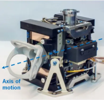
Nowadays, weather forecasting is becoming increasingly dependent on satellite data. The observations from the 63 meteorological satellites currently in operation (according to NASA data center) are crucial for monitoring weather and climate change. In order to provide reliable and increasingly accurate information, the European Organisation for the Exploitation of Meteorological Satellites (EUMETSAT) will launch six new Meteosat Third Generation (MTG) satellites from 2019. The Infra-Red Sounder (IRS) on-board of MTG will provide unprecedented high resolution data on humidity and temperature of the atmosphere. A critical subsystem of the IRS is the Corner Cube Mechanism (CCM) depicted in Fig. 1. In order to create the necessary optical path difference between both arms of the IRS interferometer, the function of the CCM is to displace linearly one of the two corner cube reflectors. This motion needs to be controlled to a level of accuracy higher than the measured wavelength. The CCM is based on a successful design developed for the Infrared Atmospheric Sounding Interferometers (IASI) currently on-board of the Metop satellites [1]. The IASI design has been modified to meet the MTG specifications [2].
The control of the linear motion of the reflector offers many challenges. First of all, a high performance in speed control is required. For the CCM system, this means that the control bandwidth needs to be higher than the main resonance frequency. Second, a parametric model for con-troller design is not available. The only available model is a finite element model (FEM). Third, the system is subject to external periodic disturbances in multiple frequencies which
1Etienne Thalmann and Yves-Julien Regamey are with the Swiss Center
for Electronics and Microtechnology (CSEM), Neuchˆatel, Switzerland
2 Alireza Karimi is with the Automatic Control Laboratory of Ecole
Polytechnique F´ed´erale de Lausanne (EPFL), Lausanne, Switzerland
Fig. 1. CCM CAD model with dummy corner cube reflector and axis needing to be controlled
need to be attenuated to attain the desired speed accuracy. Periodic disturbance rejection problem is commonly seen in systems such as hard disks [3], optical disk drives [4], active suspension systems [5] and helicopter rotor blades [6]. Disturbance rejection control of voice coil actuator for precision mechanisms has already been studied in [7].
A large closed-loop bandwidth leads to increase of the magnitude of the sensitivity function in high frequencies according to the Bode sensitivity integral [8]. The periodic disturbances are also in these frequencies, so they will be amplified in the closed-loop operation. The internal model principle can hardly be used because by reducing the mag-nitude of the sensitivity function to zero at disturbance frequencies, the infinity-norm of the sensitivity function will be increased because of the “waterbed” effect, and the system will loose its robustness and may become unstable.
The controller that is already implemented on the system is a classical PID controller with additional notch filters (called PID+N for further reference). The notch filters are designed such that their gain at disturbance frequencies is very close to zero. In other words, the notch filters open the loop at disturbance frequencies, so the disturbances will not be amplified nor attenuated by the closed-loop system. However, this controller does not satisfy the specifications on speed accuracy and should be replaced with a more advanced controller with robust performance that can attenuate the disturbances as well.
The H∞ method, used in this paper, is able to design fixed-order controllers with constraints on the magnitudes of all closed-loop sensitivity functions. In fact, there is no need to compute weighting filters as rational transfer functions like in other classical robust control methods. Moreover, only the
frequency response of the plant model is used to compute the controller parameters by a convex optimization algorithm. A public-domain toolbox for robust controller design in the frequency domain [9] is used to compute the controller, which guarantees performance, robustness and stability.
The performance of theH∞controller is compared to that of the existing PID+N. Tests are performed first in simulation using a Simulink scheme based on the finite element model and second on a test platform using the actual mechanism.
The paper is organized as follows: Section 2 describes the system and the control specifications. The frequency domain
H∞ optimization method is exposed. Section 3 presents the simulation results and the experimental results are exposed in Section 4. Finally, Section 5 gives some concluding remarks.
II. CONTROLLERDESIGNMETHOD
In this section, the control design method proposed in [10], is briefly recalled and it is shown that how H∞ constraints on the weighted sensitivity functions can be represented by linear or convex constraints.
A. Controller structure
A fixed-order linearly parametrized discrete-time con-troller is used in the optimization process and is given by:
K(z−1, ρ) =ρTφ(z−1) (1)
whereρT = [ρ1, ρ2, ...ρn]represents the vector of controller
parameters and
φT(z−1) =F(z−1)[φ1(z−1), φ2(z−1), ..., φn(z−1)] (2)
represents the vector of n stable transfer functions. These functions are defined a priori as basis functionsφimultiplied
by the fixed part of the controller F(z−1), which can be
chosen according to internal model principle to reject the disturbance frequencies (e.g. integrator). In this application, Laguerre basis functions are used [11].
Linearly parametrized controllers are used such that every point on the Nyquist diagram of the open-loop transfer function L(e−jω) becomes a linear function of the vector
of controller parametersρ:
L(e−jω) =ρTφ(e−jω)G(e−jω). (3) whereG(e−jω), the frequency response of the plant model,
is assumed to have a bounded ∞-norm. The linearity of the open-loop transfer function helps obtaining a convex parametrization of fixed-orderH∞controllers.
B. Stability and performance constraints
Let the output sensitivity function S(s) = [1 +L(s)]−1
be defined. A standard control problem is to satisfy the following nominal performance condition [8]:
kW1S(ρ)k∞<1, (4)
whereW1 represents the performance weighting filter. This
condition is equivalent to :
|W1(e−jω)|<|1 +L(e−jω, ρ)|, ∀ω. (5)
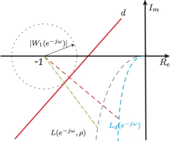
Fig. 2. Linearized nominal performance constraint
which is not a convex constraint. The method used here is based on the linearization of this constraint around a known desired open-loop transfer functionLd(e−jω). This leads to
the following linear constraint (see [10] for details):
|W1(e−jω)||1 +Ld(e−jω)|−
Re{[1 +L(e−jω, ρ)][1 +Ld(ejω)]}<0, ∀ω.
(6) This is depicted graphically in Fig. 2. The constraint is equivalent to saying that L(e−jω) has to lie under d for
all ω, where d is tangent to the performance disk of ra-dius |W1(e−jω)| and orthogonal to the segment between Ld(e−jω) and the critical point -1. This is a sufficient
con-dition of theH∞ performance constraint, which is satisfied if and only if there is no intersection between the open-loop curve and the performance disk.
Moreover, it can be shown that the number of encir-clements of the critical point by L is equal to that of
Ld. Thus, if Ld satisfies the Nyquist criterion, closed-loop
stability is guaranteed. As a result, in the case where the controller or the plant are unstable, Ld should contain the
unstable poles and zeros of of the open-loop model. The choice of Ld influences the obtained solution, closerLd to Lwill reduce the conservatism of the approach. An iterative method can be used in which, Ld for the next iteration is
chosen equal toLof the current iteration. The choice ofLd
is discussed for the specific problem treated in this paper. In the same way,H∞constraints are specified for the other sensitivity functions. For example a constraints in the input sensitivity functionU(s) =K(s)/[1 +L(s)]defined as:
kW3U(ρ)k∞<1, (7)
is convexified in an analogous way as:
|W3(e−jω)K(e−jω, ρ)||1 +Ld(e−jω)|− Re{[1 +L(e−jω, ρ)][1 +Ld(ejω)]}<0, ∀ω.
(8) The weighting frequency functionsW1(e−jω)andW3(e−jω)
are chosen such thatW1−1andW3−1provide an upper bound template forU andS, respectively. The minimum value of
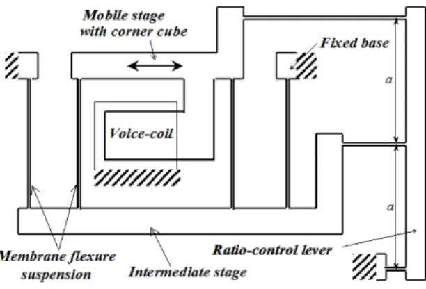
Fig. 3. Operating principle of CCM mobile stage
critical point in the Nyquist plot. This value, called modulus margin, is a good indicator for robustness.
C. Optimization problem
The performance can be improved by minimizing the upper bound of the infinity norm of the weighted sensitivity functions. This optimization can be solved by an iterative bisection algorithm described in [10].
The constraints in (6) and (8) should be satisfied for all frequencies up to the Nyquist frequency. This would lead to an infinite number of constraints. The optimization is thus performed over a finite grid of frequencies. The grid is chosen dense enough that no points of the solution violates the constraints.
III. SYSTEMDESCRIPTION ANDCONTROL SPECIFICATIONS
The system consists of a mobile mass (mainly the reflec-tor) translating along one horizontal axis shown in Fig. 1. The motion is constrained by guiding blades using the flexural structure technology developed by CSEM. This allows for high-accuracy linear guiding without any sliding surfaces or bearings. An intermediate stage, counterbalances the parasitic displacement in the blade direction (see Fig. 3). A controller is needed to accurately position the reflector using a voice coil actuator. The position is measured using a laser interferometer. Some simulations using the FEM are performed to obtain the frequency response of the system.
A. Control specifications
The controller has to fulfill mainly three tasks: 1) Control The X-axis position of the CCM in order to have good trajectory tracking. 2) Attenuate external perturbations so as to satisfy the speed accuracy specifications. 3) Limit the forces exported to the surrounding instruments.
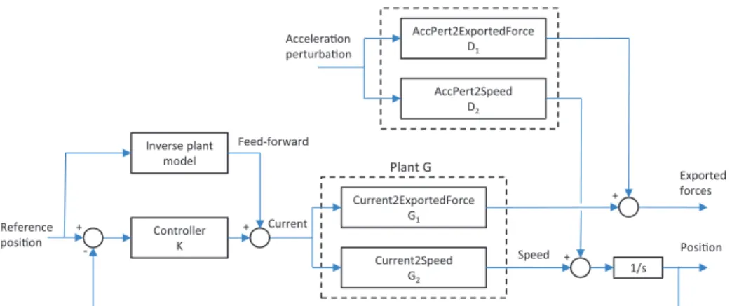
The controller design process in order to achieve these three goals is described respectively in the three sections below. The block diagram of the controlled system is de-picted in Fig. 4. The position is the main control output. The speed accuracy during the motion of the mechanism has to be guaranteed. Speed accuracy requirement during constant speed part of trajectory with micro-vibration disturbances is
specified as follows: Instantaneous speed error lower than 0.25 mm/s and RMS value of speed error computed lower than 0.06 mm/s.
The forces exported by the actuation of the voice coil should be minimized, although it is not the main control objective. A feed-forward signal based on an inverse plant model is applied to reduce the tracking error. For the latter, a 2nd order plant model approximation is used.
1) Position control of the Corner Cube: The CCM trans-fer function from the voice coil current to the output position (G2/s) has a main resonance frequency around 5 Hz and
other modes at much higher frequency (see Fig. 5). It can basically be approximated by a second order spring-mass system. One of the control challenges that arises is that the main resonance peak is below the desired control bandwidth (a bandwidth of at least 10 Hz is required).
A solution could be to cancel the poles causing the first resonance peak. This can be done by adding zeros equal to the poles causing the resonance in the fixed part F(z−1)
of the controller in (2). In practice, however, this is not a good solution because it is not robust at all. A slight offset between the cancelled frequency and the real resonance frequency results in an oscillation. A more robust alternative is to place complex conjugate zeros in the fixed part of the controllerF(z−1)at a frequency close to the resonance but
with a much greater damping ratio (ζ≈0.7). This damps the resonance peak without canceling it in open-loop and results in no oscillation once the loop is closed. An integrator is also considered inF(z−1)to have zero steady-state error.
Since the design method is sensitive to the choice of
Ld(e−jω), this function has to be close to L(e−jω, ρ) in
order to get the desired controller.Ld(e−jω)is designed such
that it corresponds to a 2nd order system with a controller consisting of an integrator and a pair of critically damped zeros (ζ = 1) at resonance frequency. It is obtained by combining the dominant poles of the plant model, a pole in
z= 1 and two zeros in z =e−2πFresTs, where F
res is the
frequency of the dominant poles andTsis the sampling time.
The gain is adjusted to get the desired crossover frequency.
2) External disturbance attenuation: Neighboring instru-ments, that will be present in the satellite, inject micro-vibrations at the base of the mechanism. This disturbance is a linear combination of cryocooler system (CCS) and reaction wheel perturbations. The CCS micro-vibrations are permanently present on the X axis at multiples of a de-fined frequency (FCCS = 57.5 Hz) with different specified
amplitudes. The reaction wheel disturbance consists of a sum of micro-vibrations coming from 22 different frequency sub-bands with the following characteristics: 1) One single frequency per sub-band is injected. 2) For each sub-band, the injected frequency is swept such as the entire sub-bands are covered during the entire experiment (100 s, simultaneous sweep). 3) The initial phases between each injected frequency (22 in total) are random.
The reaction wheel disturbance is acting on the 3 axes of the system but only the X axis is considered here as it is the only controllable one. The disturbances enter the system
Current Controller K Plant G Current2ExportedForce G1 Current2Speed G2 1/s Reference posi!on AccPert2ExportedForce D1 AccPert2Speed D2 Accelera!on perturba!on Exported forces Speed + + + - Posi!on Inverse plant model + Feed-forward
Fig. 4. Block diagram of the control problem
Magnitude (dB)-150 -100 -50 0 100 101 102 103 Phase (deg) -1800 -1440 -1080 -720 -360 0
Transfer function from current input to CCM position
Frequency (Hz)
Fig. 5. Bode plot of transfer function from current to position, obtained by spectral analysis
as accelerations. The FEM-obtained transfer functions D1
and D2 (see Fig. 4) give respectively the resulting force
perturbations at the base of the mechanism and the speed perturbation at the mobile part of the CCM. The effect of the cumulated perturbations on the speed along the X axis can be seen on the spectrum depicted in Fig. 6. The CCS perturbation is significantly larger than the one created by reaction wheel.
In order to attenuate the external perturbations, constraints are set on the output sensitivity function S at selected fre-quencies summarized in Table I. Since the output sensitivity function is the transfer function between disturbance and output, there will be attenuation in the ranges where its magnitude is below 0 dB. By setting respectively a -2 dB and -3 dB constraint on CSS frequencies 2 and 7, the corresponding disturbances are multiplied by a factor 0.8 and 0.7. These perturbations where chosen because they have the greatest amplitudes along with the 3rdone (see Fig. 6). The
values of the constraints were chosen so as to attenuate the disturbances enough without making the problem infeasible. Another method, described further, is used for the 3rd CSS
frequency. For the 1st frequency, the constraint is set to 0 dB which makes sure that the disturbance is not amplified.
Frequency (Hz) 0 100 200 300 400 500 600 |Perturbation on speed (m/s)| ×10-5 0 1 2 3 4 5 6 7 FFT of speed perturbation
Fig. 6. Speed perturbation in frequency domain TABLE I OPTIMIZATION CONSTRAINTS Frequenciesf (Hz) Constraint 0 - 20 kS(e−j2πf)k<0dB 57.5 (= 1·FCCS) kS(e−j2πf)k<0dB 115 (= 2·FCCS) kS(e−j2πf)k<−2dB 402.5 (= 7·FCCS) kS(e−j2πf)k<−3dB 210 - 220 kU(e−j2πf)k<80dB 700 - 1000 kU(e−j2πf)k<80dB
Since its amplitude is lower, this is sufficient to satisfy the specifications. Rejecting more frequencies would be possible but it would increase the order of the controller (already equal to 18) and is not necessary to satisfy the specifications. The disturbance rejection bandwidth is also pushed higher by constraining the output sensitivity function to stay below 0 dB up to 20 Hz. Increasing the bandwidth increases the range of low frequency perturbations that can be attenuated. For robustness, a modulus margin of 0.45 is specified. This corresponds to the margin of the existing controller and guarantees that the robustness is not decreased. The constraints and the resulting output sensitivity function are depicted in Fig. 7.
3) Exported forces limitation: The transfer function G1
from current to exported force along axis X obtained by FEM is depicted in Fig. 8. The product ofU timesG1corresponds
100 101 102 103 Ma g n it u d e (d B) -30 -20 0 -10 0 10 S H∞ S PID+N S constraint Output sensitivity function
Frequency (Hz)
Fig. 7. Magnitude plot of output sensitivity functionSofH∞controller with constraints and PID+N controller
Ma g n it u d e (d B) -40 -20 0 20 100 101 102 103
Transfer function from current to exported force
Frequency (Hz)
Fig. 8. Bode plot of transfer function from current to exported force
to the transfer function from position disturbance to exported forces (see Fig. 4). In order to limit the exported forces caused by the disturbance, the input sensitivity function U
can be limited at frequencies where the amplitude ofG1 is
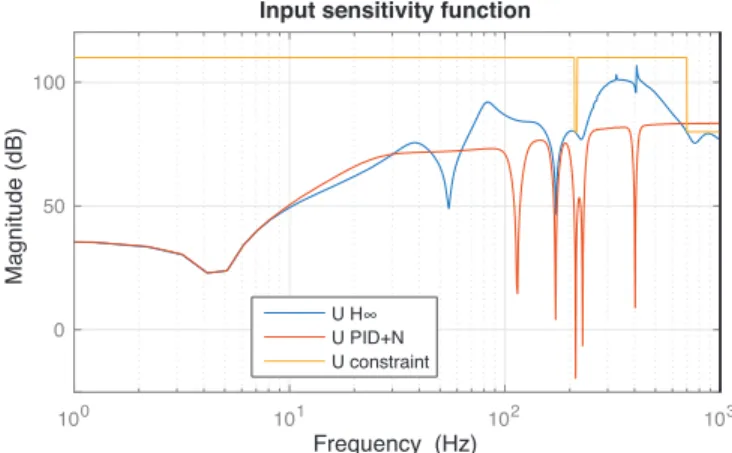
high. A limitation on the amplitude ofU is thus set around the 215 Hz resonance ofG1. The constraint is set to 80 dB.
Using a lower value would decrease the exported forces but impacts the overall controller performance negatively. The forces that are directly exported due to the perturbations through D1 cannot be controlled since there is no feedback
on this output.
A pair of zeros with very low damping ratio is also placed at the 3rdCCS frequency. This has the same effect as a notch filter: it cancels this frequency at the input of the plant. This can be seen in the amplitude of U at 172.5 Hz in Fig. 9. The disturbance is neither amplified nor attenuated which has the same effect on S as constraining it to 0 dB. The advantage here is that the cancellation of this frequency at plant input causes no force to be exported. This is ideal for this perturbation which is close to the exported force resonance frequency.
To avoid important high frequency noise amplification, which worsens the speed accuracy, a constraints on|U|above 700 Hz is considered. The resulting input sensitivity function is depicted in Fig. 9. The obtained controller and closed-loop transfer functions are depicted in Fig. 10.
IV. SIMULATION ANDEXPERIMENTALRESULTS
a) PID+Notch controller: The controller that is already implemented on the system is a classical PID controller with
100 101 102 103 Ma g n it u d e (d B) 0 50 100 U H∞ U PID+N U constraint
Input sensitivity function
Frequency (Hz)
Fig. 9. Magnitude plot of input sensitivity functionU ofH∞ controller with constraints and PID+N controller
Ma g n it u d e (d B) -100 -50 0 50 100 150 100 101 102 103 CL H∞ CL PID+N H∞ controller
Closed-loop and controller transfer functions
Frequency (Hz)
Fig. 10. Bode plot ofH∞ controller and closed-loop transfer functions withH∞and PID+N controllers
additional notch filters. The PID part is designed using a 2nd order physical model approximation. The coefficients are obtained through state-space pole placement from [12] so as to obtain the closed-loop poles of a low pass filter with chosen bandwidth. Fourth order notch filters are placed at CSS frequencies 2, 3, 4 and 7. There is an additional filter at the exported force resonance frequency (215 Hz). Their effect can be seen on S and U. The frequencies are cancelled at the plant input as shown by the small magnitude ofU at corresponding frequencies in Fig. 9. As a result, the disturbances are transferred to the output without modification, which can be seen from the 0 dB value of S
at the corresponding frequencies in Fig. 7.
Here the advantages of the H∞ method compared to notch filters can be seen. First, the output sensitivity function can be brought lower than 0 dB at desired frequencies which means that the disturbance can be attenuated. Second, the output sensitivity function can be set to 0 dB for the first CSS frequency. Since this perturbation is close to the bandwidth frequency, it is not possible to place a notch filter there without reducing the phase margin significantly. As a result, the PID+N controller amplifies this disturbance by a factor 1.4 (3 dB). Note, however, that because of the “waterbed effect”, theH∞controller has greater disturbance amplification outside of the targeted frequencies.
b) Simulation results: The controller is first simulated over 100 seconds using the FEM and the specified external
Time (s)
0 20 40 60 80
Instantaneous speed error (mm/s)
-0.3 -0.2 -0.1 0 0.1 0.2 PID+N H∞
Fig. 11. Absolute speed error with H∞ and PID+N controller in simulation. Specified bounds are marked in red.
perturbations. The reference trajectory has the following characteristics: continuous operation; triangular symmetric
±5 mm peak to peak trajectory; exponential acceleration and 20s period. The speed accuracy criteria are measured and compared with the requirements. The RMS of speed error with the new controller is 0.058, which satisfies the 0.06 specification. The instantaneous speed error depicted in Fig. 11 is also within the specified 0.25 mm/s bounds. The PID+N controller on the other hand could only achieve an RMS error of 0.076 and the instantaneous speed error in Fig. 11 violates the bounds in several points.
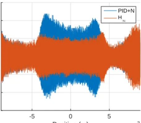
c) Experimental results: Experiments are performed on the CCM in a clean room environment. The system is placed on a vibration isolated table. A shaker is used to simulate the disturbance of the CCS. The position is measured during one back and forth motion with an interferometer which has a resolution of 2 nm. The trajectory has the characteristics described in Section IV but its amplitude is 9 mm peak to peak and the period is 35 s. The ratio between amplitudes of perturbation at different CCS frequencies is chosen according to the specifications but the absolute amplitude of the distur-bance does not correspond to the specifications. This is due to the fact that the transfer function between the current in the shaker and the accelerations at the feet of the mechanism is unknown. As a result, experiments could not be used to verify requirements on the speed error but they are used to compare controllers.
The experimental speed error for PID+N and H∞ con-trollers is shown in Fig. 12. The simulation results are confirmed: TheH∞controller is better at attenuating pertur-bations. The RMS speed error is 0.038 mm/s with the PID+N and 0.028 mm/s with theH∞controller. It is also interesting to notice that the error changes significantly with position. It makes sense that the characteristics of the system change as the mass is displaced. This could be taken into account for further controller design.
V. CONCLUSIONS
The frequency-domainH∞controller design method pro-posed in this article made it possible to design a controller which satisfies the speed accuracy specifications. This could
Position (m) ×10-3 -5 0 5 Speed error (mm/s) -0.15 -0.1 -0.05 0 0.05 0.1 0.15 PID+N H∞
Fig. 12. Absolute speed error with H∞ and PID+N controller in experiment with shaker
not be obtained by the classical PID controller with notch filters. The experimental results also proved that the H∞ controller is better at attenuating the external perturbations than the existing controller and that the speed accuracy is improved. The effectiveness of the proposed data-driven for shaping the sensitivity functions in the frequency domain is well illustrated via a challenging application.
REFERENCES
[1] D. Simeoni, P. Astruc, D. Miras, C. Alis, O. Andreis, D. Scheidel, C. Degrelle, P. Nicol, B. Bailly, P. Guiard et al., “Design and development of IASI instrument,” inOptical Science and Technology, the SPIE 49th Annual Meeting. International Society for Optics and Photonics, 2004, pp. 208–219.
[2] P. Spanoudakis, P. Schwab, L. Kiener, H. Saudan, and G. Perruchoud, “Development Challenges of Utilizing a Corner Cube Mechanism Design with Successful IASI Flight Heritage for the Infrared Sounder (IRS) on MTG; Recurrent Mechanical Design not Correlated to Recurrent Development,” in16th European Space Mechanisms and Tribology Symposium, Sep. 2015.
[3] K. Chew and M. Tomizuka, “Digital control of repetitive errors in disk drive systems,”Control Systems Magazine, IEEE, vol. 10, no. 1, pp. 16–20, Jan 1990.
[4] A. Sacks, M. Bodson, and P. Khosla, “Experimental results of adaptive periodic disturbance cancelation in a high performance magnetic disk drive,”ASME Journal of Dynamic Systems Measurement and Control, vol. 118, no. 3, pp. 416–424, 1996.
[5] A. Karimi and Z. Emedi, “H∞ gain-scheduled controller design for rejection of time-varying narrow-band disturbances applied to a benchmark problem,”European Journal of Control, vol. 19, no. 4, pp. 279–288, 2013.
[6] P. Arcara, S. Bittanti, and M. Lovera, “Periodic control of helicopter rotors for attenuation of vibrations in forward flight,”IEEE Trans. on Control Systems Technology, vol. 8, no. 6, pp. 883–894, 2000. [7] Q. Chen, L. Li, M. Wang, and L. Pei, “The precise modeling and active
disturbance rejection control of voice coil motor in high precision motion control system,”Applied Mathematical Modelling, pp. –, 2015. [8] C. J. Doyle, B. A. Francis, and A. R. Tannenbaum,Feedback Control
Theory. New York: Mc Millan, 1992.
[9] A. Karimi, “Frequency-domain robust control toolbox,” in52nd IEEE Conference in Decision and Control, 2013, pp. 3744 – 3749. [10] A. Karimi and G. Galdos, “Fixed-orderH∞ controller design for
nonparametric models by convex optimization,”Automatica, vol. 46, no. 8, pp. 1388–1394, 2010.
[11] P. M¨akil¨a, “Approximation of stable systems by Laguerre filters,”
Automatica, vol. 26, no. 2, pp. 333–345, 3 1990.
[12] J. Kautsky, N. K. Nichols, and P. Van Dooren, “Robust pole assignment in linear state feedback,” International Journal of Control, vol. 41, no. 5, pp. 1129–1155, 1985.