Documentation for the TIMES Model
PART II
April 2005
Authors:
Richard Loulou
Antti Lehtilä
Amit Kanudia
Uwe Remne
Gary Goldstein
This documentation is composed of thee Parts.
Part I comprises eight chapters constituting a general description of the TIMES paradigm, with emphasis on the model’s general structure and its economic significance. Part I also includes a simplified mathematical formulation of TIMES, a chapter comparing it to the MARKAL model, pointing to similarities and differences, and chapters describing new model options.
Part II comprise 7 chapters and constitutes a comprehensive reference manual intended for the technically minded modeler or programmer looking for an in-depth understanding of the complete model details, in particular the relationship between the input data and the model mathematics, or contemplating making changes to the model’s equations. Part II includes a full description of the sets, attributes, variables, and equations of the TIMES model.
Part III describes the GAMS control statements required to run the TIMES model. GAMS is a modeling language that translates a TIMES database into the Linear Programming matrix, and then submits this LP to an optimizer and generates the result files. In addition to the GAMS program, two model interfaces (VEDA-FE and VEDA-BE) are used to create, browse, and modify the input data, and to explore and further process the model’s results. The two VEDA interfaces are described in detail in their own user’s guides.
1 INTRODUCTION ... 8
1.1 Basic notation and conventions ... 8
1.2 GAMS modelling language and TIMES implementation ... 9
2 SETS ... 10
2.1 Indexes (One-dimensional sets) ... 10
2.2 User input sets ... 15
2.2.1 Definition of the Reference Energy System (RES) ... 15
2.2.1.1 Processes ... 16
2.2.1.2 Commodities ... 20
2.2.2 Definition of the time structure ... 20
2.2.2.1 Time horizon ... 20
2.2.2.2 Timeslices ... 22
2.2.3 Multi-regional models ... 23
2.2.4 Overview of all user input sets ... 26
2.3 Definition of internal sets ... 32
3 PARAMETERS ... 38
3.1 User input parameters ... 38
3.1.1 Inter- and extrapolation of user input parameters ... 38
3.1.2 Inheritance and aggregation of timesliced input parameters ... 42
3.1.3 Overview of user input parameters ... 44
3.2 Internal parameters ... 107 3.3 Report parameters ... 118 4 VARIABLES ... 125 4.1 VAR_ACT(r,v,t,p,s) ... 128 4.2 VAR_BLND(r,ble,opr) ... 129 4.3 VAR_CAP(r,t,p) ... 129 4.4 VAR_COMNET(r,t,c,s) ... 129 4.5 VAR_COMPRD(r,t,c,s) ... 129 4.6 VAR_DNCAP(r,t,p,u) ... 129 4.7 VAR_ELAST(r,t,c,s,j,l) ... 130 4.8 VAR_FLO(r,v,t,p,c,s) ... 130 4.9 VAR_IRE(r,v,t,p,c,s,ie) ... 130 4.10 VAR_NCAP(r,v,p) ... 131
4.11 VAR_OBJ(y0) and related variables ... 132
4.11.1 VAR_OBJR(r, y0)... 132
4.11.2 INVCOST(r,y) ... 132
4.11.3 INVTAXSUB(r,y) ... 132
4.13 Variables used in User Constraints ... 134 4.13.1 VAR_UC(uc_n) ... 134 4.13.2 VAR_UCR(uc_n,r) ... 135 4.13.3 VAR_UCT(uc_n,t) ... 135 4.13.4 VAR_UCRT(uc_n,r,t) ... 135 4.13.5 VAR_UCTS(uc_n,t,s) ... 135 4.13.6 VAR_UCRTS(uc_n,r,t,s) ... 135 4.13.7 VAR_UCSU(uc_n,t) ... 135 4.13.8 VAR_UCSUS(uc_n,t,s) ... 135 4.13.9 VAR_UCRSUS(r,uc_n,r,t,s) ... 135 4.13.10 VAR_UCRSU(uc_n,r,t) ... 135 5 EQUATIONS ... 136 5.1 Notational conventions ... 136
5.1.1 Notation for summations ... 136
5.1.2 Notation for logical conditions ... 137
5.1.3 Using Indicator functions in arithmetic expressions ... 137
5.2 Objective function EQ_OBJ ... 138
5.2.1 Introduction and notation ... 138
5.2.1.1 Notation relative to time ... 139
5.2.1.2 Other notation ... 140
5.2.1.3 Reminder of some technology attribute names (each is indexed by t) ... 140
5.2.1.4 Discounting option... 140
5.2.1.5 Components of the Objective function ... 140
5.2.2 Investment costs: INVCOST(y) ... 141
5.2.3 Taxes and subsidies on investments ... 148
5.2.4 Decommissioning (dismantling) capital costs: COSTDECOM(y) ... 148
5.2.5 Fixed annual costs: FIXCOST(y), SURVCOST(y) ... 153
5.2.6 Annual taxes/tubsidies on capacity: FIXTAXSUB(Y) ... 160
5.2.7 Variable annual costs VARCOST(y), y ≤ EOH ... 160
5.2.8 Cost of demand reductions ELASTCOST(y) ... 161
5.2.9 Salvage value: SALVAGE (EOH+1) ... 161
5.2.10 Late revenues from endogenous commodity recycling after EOH LATEREVENUE(y) ... 169
5.2.11 The two discounting methods for annual payments ... 170
5.3 Constraints ... 172
5.3.1 Equation: EQ_ACTFLO ... 174
5.3.2 Equation EQ(l)_ACTBND ... 175
5.3.3 Equation: EQ(l)_BLND ... 176
5.3.4 Bound: BND_ELAST ... 177
5.3.5 Equation: EQ(l)_BNDNET/PRD ... 178
5.3.6 Equation: EQ(l)_CAPACT ... 179
5.3.7 Equation: EQ(l)_CPT ... 184
5.3.8 Equation: EQ(l)_COMBAL ... 186
5.3.9 Equation: EQE_COMPRD ... 195
5.3.10 Equation: EQ(l)_CUMNET/PRD ... 196
5.3.11 Equation EQ_DSCNCAP ... 198
5.3.12 Equation: EQ_DSCONE ... 199
5.3.13 Equation: EQ(l)_FLMRK ... 200
5.3.14 Equation: EQ(l)_FLOBND ... 203
5.3.15 Equation: EQ(l)_FLOFR ... 205
5.3.20.1 EQ_SRGTSS: Storage between timeslices (including night-storage devices): ... 230
5.3.20.2 EQ_STGIPS: Storage between periods ... 231
5.3.21 Equations: EQ(l)_STGIN / EQ(l)_STGOUT ... 232
5.3.22 User Constraints ... 233
5.3.22.1 Equation: EQ(l)_UC / EQE_UC ... 247
5.3.22.2 Equation: EQ(l)_UCR / EQE_UCR ... 248
5.3.22.3 Equation: EQ(l)_UCT / EQE_UCT ... 249
5.3.22.4 Equation: EQ(l)_UCRT / EQE_UCRT ... 250
5.3.22.5 Equation: EQ(l)_UCRTS / EQE_UCRTS ... 251
5.3.22.6 Equation: EQ(l)_UCTS / EQE_UCTS ... 252
5.3.22.7 Equation: EQ(l)_UCSU / EQE_UCSU ... 260
5.3.22.8 Equation: EQ(l)_UCRSU / EQE_UCRSU ... 262
5.3.22.9 Equation: EQ(l)_UCRSUS / EQE_UCRSU ... 264
5.3.22.10 Equation: EQ(l)_UCSUS / EQE_UCSUS ... 266
5.3.22.11 Equation: EQ(l)_UCSU / EQE_UCSU ... 271
5.3.22.12 Equation: EQ(l)_UCRSU / EQE_UCRSU ... 273
5.3.22.13 Equation: EQ(l)_UCRSUS / EQE_UCRSU ... 275
5.3.22.14 Equation: EQ(l)_UCSUS / EQE_UCSUS ... 277
6 THE ENDOGENOUS TECHNOLOGICAL LEARNING (ETL) OPTION ... 279
6.1 Sets, Switches and Parameters ... 279
6.2 Variables ... 285 6.2.1 VAR_CCAP(r,t,p) ... 286 6.2.2 VAR_CCOST(r,t,p) ... 286 6.2.3 VAR_DELTA(r,t,p,k) ... 287 6.2.4 VAR_IC(r,t,p) ... 287 6.2.5 VAR_LAMBD(r,t,p,k) ... 288 6.3 Equations ... 289 6.3.1 EQ_CC(r,t,p) ... 291 6.3.2 EQ_CLU(r,t,p) ... 292 6.3.3 EQ_COS(r,t,p) ... 293 6.3.4 EQ_CUINV(r,t,p) ... 295 6.3.5 EQ_DEL(r,t,p) ... 296 6.3.6 EQ_EXPE1(r,t,p,k) ... 297 6.3.7 EQ_EXPE2(r,t,p,k) ... 298 6.3.8 EQ_IC1(r,t,p)... 299 6.3.9 EQ_IC2(r,t,p)... 300 6.3.10 EQ_LA1(r,t,p,k) ... 301 6.3.11 EQ_LA2(r,t,p,k) ... 302 6.3.12 EQ_OBJSAL(r,cur) ... 303 6.3.13 EQ_OBJINV(r,cur) ... 304
7 THE TIMES CLIMATE MODULE ... 305
7.1 Formulation of the TIMES Climate Module ... 305
7.1.1 Approach taken ... 305
7.1.1.1 Concentrations (accumulation of CO2) ... 306
7.1.1.2 Radiative forcing ... 306
7.1.1.3 Temperature increase ... 307
7.2 Input parameters of the Climate Module ... 308
7.4.4 Equation: EQ_CO2LOW ... 313 7.4.5 Equation: EQ_MXCONC ... 315 7.5 Reporting Parameters... 316 7.5.1 DT_FORC ... 316 7.5.2 DT_ATM ... 317 7.5.3 DT_LOW ... 318
7.6 Default values of the climate parameters ... 320
7.7 GAMS implementation ... 321
7.7.1 Specification of parameters ... 321
7.7.2 Climate related Variables ... 323
7.7.3 Equations ... 323
7.7.4 Example of use ... 324
7.7.5 Exporting results to VEDA4... 324
The purpose of the Reference Manual is to lay out the full details of the TIMES model, including data specification, internal data structures, and mathematical formulation of the model’s Linear Program (LP) formulation, as well as the Mixed Integer Programming (MIP) formulations required by some of its options. As such, it provides the TIMES modeller/programmer with sufficiently detailed information to fully understand the nature and purpose of the data components, model equations and variables. A solid understanding of the material in this Manual is a necessary prerequisite for anyone considering making programming changes in the TIMES source code.
The Reference Manual is organized as follows:
Chapter 1 Basic notation and conventions: lays the groundwork for understanding the rest of the material in the Reference Manual;
Chapter 2 Sets: explains the meaning and role of various sets that identify how the model components are grouped according to their nature (e.g. demand devices, power plants, energy carriers, etc.) in a TIMES model;
Chapter 3 Parameters: elaborates the details related to the user-provided numerical data, as well as the internally constructed data structures, used by the model generator (and report writer) to derive the coefficients of the LP matrix (and prepare the results for analysis);
Chapter 4 Variables: defines each variable that may appear in the matrix, both explaining its nature and indicating how if fits into the matrix structure;
Chapter 5 Equations: states each equation in the model, both explaining its role, and providing its explicit mathematical formulation;
Chapter 6 The User Constraints: explains the framework that may be employed by modellers to formulate additional linear constraints, which are not part of the generic constraint set of TIMES, without having to bother with any GAMS programming;
Chapter 7 The Lumpy Investment facility, and
Chapter 8 The Endogenous Technological Learning capability.
1.1
Basic notation and conventions
To assist the reader, the following conventions are employed consistently throughout this chapter:
• Sets, and their associated index names, are in lower and bold case, e.g., com is the set of all commodities;
• Literals, explicitly defined in the code, are in upper case within single quotes, e.g., ‘UP’ for upper bound;
• Parameters, and scalars (constants, i.e., un-indexed parameters) are in upper case, e.g., NCAP_AF for the availability factor of a technology;
• Variables are in upper case with a prefix of VAR_, e.g., VAR_ACT corresponds to the activity level of a technology.
1.2
GAMS modelling language and TIMES implementation
TIMES consists of generic variables and equations constructed from the specification of sets and parameter values depicting an energy system for each distinct region in a model. To construct a TIMES model, a preprocessor first translates all data defined by the modeller into special internal data structures representing the coefficients of the TIMES matrix applied to each variable of Chapter 4 for each equation of Chapter 5 in which the variable may appear. This step is called Matrix Generation. Once the model is solved (optimised) a Report Writer assembles the results of the run for analysis by the modeller. The matrix generation, report writer and control files are written in GAMS1 (the General Algebraic Modelling System), a powerful high-level language specifically designed to facilitate the process of building large-scale optimisation models. GAMS accomplishes this by relying heavily on the concepts of sets, compound indexed parameters, dynamic looping and conditional controls, variables and equations. Thus there is very a strong synergy between the philosophy of GAMS and the overall concept of the RES specification embodied in TIMES making GAMS very well suited to the TIMES paradigm.
Furthermore, by nature of its underlying design philosophy, the GAMS code is very similar to the mathematical description of the equations provided in Chapter 5. Thus, the approach taken to implement a TIMES model is to “massage” the input data by means of a (rather complex) preprocessor that handles the necessary exceptions that need to be taken into consideration to properly construct the matrix coefficients in a form ready to be applied to the appropriate variables in the respective equations. GAMS also integrates seamlessly with a wide range of commercially available optimisers that are charged with the task of solving the actual TIMES linear (LP) or mixed integer (MIP) problems that represent the desired model. This step is called the Solve or Optimisation step. CPLEX or XPRESS are the optimisers most often employed to solve the TIMES LP and MIP formulations.
The standard TIMES formulation has optional features, such as lumpy investments and endogenous technology learning. In addition, a modeller experienced in GAMS programming and the details of the TIMES implementation can define additional equation modules or report routine modules based on an extension mechanism, which allows the linkage of these modules to the standard TIMES code in a flexible way (see PART III, chapter 3)
To build, run and analyse a TIMES model several software tools have been developed in the past or are currently under development, so that the modeller does not need to provide the input information needed to build a TIMES model directly in GAMS. These tools are the model interfaces VEDA-FE, ANSWER-TIMES as well as the reporting and analysing tool VEDA-BE.
specifying qualitative characteristics of the energy system. One can distinguish between one-dimensional and multi-one-dimensional sets. The former sets contain single elements, e.g. the set
prc contains all processes of the model, while the elements of multi-dimensional sets are a combination of one-dimensional sets. An example for a multi-dimensional set is the set top, which specifies for a process the commodities entering and leaving that process.
Two types of sets are employed in the TIMES framework: user input sets and internal sets. User input sets are created by the user, and used to describe qualitative information and characteristics of the depicted energy system. One can distinguish the following functions associated with user input sets:
• definition of the elements or building blocks of the energy system model (i.e. regions, processes, commodities),
• definition of the time horizon and the sub-annual time resolution,
• definition of special characteristics of the elements of the energy system.
In addition to these user sets, TIMES also generates its own internal sets. Internal sets serve to both ensure proper exception handling (e.g., from what date is a technology available, or in which time-slices is a technology permitted to operate), as well as sometimes just to improve the performance or smooth the complexity of the actual model code.
In the following sections, the user input sets and the internal sets will be presented. A special type of set is an one-dimensional set, also called index, which is needed to build multi-dimensional sets or parameters. At the highest level of the one-multi-dimensional sets are the master or “domain” sets that define the comprehensive list of elements (e.g., the main building blocks of the reference energy system such as the processes and commodities in all regions) permitted at all other levels, with which GAMS performs complete domain checking, helping to automatically ensure the correctness of set definition (for instance, if the process name used in a parameter is not spelled correctly, GAMS will issue a warning). Therefore, before elaborating on the various sets, the indexes used in TIMES are discussed.
2.1
Indexes (One-dimensional sets)
Indexes (also called one-dimensional sets) contain in most cases the different elements of the energy model. A list of all indexes used in TIMES is given in Table 2. Examples of indexes are the set prc containing all processes, the set c containing all commodities or the set all_reg
containing all regions of the model. Some of the one-dimensional sets are subsets of another one-dimensional set, e.g., the set r comprising the so-called internal model regions is a subset of the set all_reg which in addition also contains the so-called external model regions2. To express that the set r depends on the set all_reg, the master set all_reg is put in brackets after the set name r: r(all_r).
The set cg comprises all commodity groups3. Each commodity c is considered as a commodity group with only one element the commodity itself. Thus the commodity set c is a subset of the commodity group set cg.
Apart from indexes that are under user control, some indexes have fixed elements to serve as indicators within sets and parameters and should not be modified by the user (Table 1). The only exception to this rule is the set prc_grp: while the process groups IRE, NST, PRV,
Set/Index name Description
bd(lim) Index of bound type; subset of the set lim having the internally fixed elements ‘LO’, ‘UP’, ‘FX’.
com_type Indicator of commodity type; initialized to the elements DEM (demand), NRG (energy), MAT (material), ENV (environment), FIN (financial), but the user can define any list for com_type in MAPLIST.DEF with the exception of the predefined elements DEM, ENV, FIN, MAT, NRG.
lim Index of limit types; internally fixed to the elements ‘LO’, ‘UP’, ‘FX’, ‘N’. ie Export/import exchange index; internally fixed to the two elements: ‘IMP’
standing for import and ‘EXP’ standing for export.
io Input/Output index; internally fixed elements: ‘IN’, ‘OUT’; used in combination with processes and commodities as indicator whether a commodity enters or leaves a process.
prc_grp List of process groups; internally established in MAPLIST:DEF as: CHP: combined heat and power plant
DISTR: distribution process DMD: demand device
ELE: electricity producing technology excluding CHP HPL: heat plant
MISC: miscellaneous
PRE: technology with energy output not falling in the group of the other energy technologies
REF: refinery process
RENEW: renewable energy technology XTRACT: extraction process.
The user may adjust this list to any disjoint groups desired. The following groups are required by the model, therefore must not be deleted by the user: IRE: inter-regional exchange process
PRV: technology with material output measured in volume units PRW: technology with material output measured in weight units NST: night (off-peak) storage process
STG: storage process STK: stockpiling process.
tslvl Index of timeslice levels; internally fixed to the elements ‘ANNUAL’, ‘SEASON’, ‘WEEKLY’, ‘DAYNITE’.
uc_grptype Index of internally fixed key types of variables: = ‘ACT_’, ‘CAP_’, ‘COMPRD_’, ‘COMCON_’, ‘FLO_’, ‘IRE_’, ‘NCAP_’, used in association with the user constraints.
uc_name List of internally fixed indicators for attributes able to be referenced as coefficients in user constraints (e.g. the flow variable may be multiplied by the attribute FLO_COST in a user constraint if desired): =
‘ACT_COST’, ‘ACT_BNDUP’, ‘ACT_BNDLO’, ‘ACT_BNDFX’, ‘CAP_BNDUP’, ‘CAP_BNDLO’, ‘CAP_BNDFX’, ‘GROWTH’, ‘FLO_COST’, ‘FLO_DELIV’, ‘FLO_SUB’, ‘FLO_TAX’,
age Index for age (number of years since installation) into a parameter shaping curve; default elements 1-200. all_r all_reg r All internal and external regions.
bd bnd_type lim Index of bound type; subset of lim, having the internally fixed elements ‘LO’, ‘UP’, ‘FX’.
c com,
com1, com2, com3
cg User defined7 list of all commodities in all regions; subset of cg.
cg com_grp, cg1, cg2, cg3, cg4
c User defined list of all commodities and commodity groups in all regions8; each commodity itself is
considered a commodity group; initial elements are the members of com_type.
com_typ e
Indicator of commodity type; initialized to the elements DEM (demand), NRG (energy), MAT (material), ENV (environment), FIN (financial), but the user can define any list for com_type in
MAPLIST.DEF with the exception of the predefined elements DEM, ENV, FIN, MAT, NRG.
cur cur User defined list of currency units.
datayear y Years for which model input data are specified. ie impexp Export/import exchange indicator; internally fixed =
‘EXP’ for exports and ‘IMP’ for imports. io inout Input/Output indicator for defining whether a
commodity flow enters or leaves a process; internally fixed = ‘IN’ for enters and ‘OUT’ for leaves.
j Indicator for elastic demand steps and sequence
number of the shape/multi curves; default elements 1-50.
kp Index for “kink” points in ETL formulation; currently limited to 1-6 {can be extended in <case>.run file by including SET KP / 1*n /; for n-kink points.
lim lim_type, l, ll
bd Index of limit types; internally fixed = ‘LO’, ‘UP’, ‘FX’ and ‘N’.
p prc User defined list of all processes in all regions9.
4
This column contains the names of the indexes as used in this document. 5
For programming reasons, alternative names (aliases) may exist for some indexes. This information is only relevant for those users who are interested in gaining an understanding of the underlying GAMS code.
6
This column refers to possible related indexes, e.g. the index c is a subset of the index
cg. 7
VEDA compiles the complete list from the union of the commodities defined in each region.
period. prc_grp
List of process groups; internally established in MAPLIST:DEF as:
CHP: combined heat and power plant DISTR: distribution process
DMD: demand device
ELE: electricity producing technology excluding CHP
HPL: heat plant MISC: miscellaneous
PRE: technology with energy output not falling in the group of the other energy technologies
REF: refinery process
RENEW: renewable energy technology XTRACT: extraction process.
The user may adjust this list to any disjoint groups desired. The following groups are required by the model and therefore must not be deleted by the user: IRE: inter-regional exchange process
PRV: technology with material output measured in volume units
PRW: technology with material output measured in weight units
NST: night (off-peak) storage process STG: storage process
STK: stockpiling process.
r reg all_r Explicit regions within the area of study. s all_ts, ts,
s2, sl
Timeslice divisions of a year, at any of the tslvl levels. t milestonyr,
tt
y Representative years for the model periods.
teg p Technologies modelled with endogenous technology
learning.
tslvl Timeslice level indicator; internally fixed =
‘ANNUAL’, ‘SEASON’, ‘WEEKLY’, ‘DAYNITE’.
u units units_com,
units_cap, units_act
List of all units; maintained in the file UNITS.DEF. uc_grpty
pe
Fixed internal list of the key types of variables: fixed = ‘ACT_’, ‘CAP_’, ‘COMPRD_’, ‘COMCON_’,
‘FLO_’, ‘IRE_’, ‘NCAP_’.
when deriving a coefficient (e.g. the flow variable may be multiplied by the attribute FLO_COST to represent expenditure associated with said flow in a user
constraint if desired): =
‘ACT_COST’, ‘ACT_BNDUP’, ‘ACT_BNDLO’, ‘ACT_BNDFX’, ‘CAP_BNDUP’, ‘CAP_BNDLO’, ‘CAP_BNDFX’, ‘GROWTH’, ‘FLO_COST’, ‘FLO_DELIV’, ‘FLO_SUB’, ‘FLO_TAX’, ‘NCAP_COST’, ‘NCAP_ITAX’, ‘NCAP_ISUB’. unit List of capacity blocks that can be added in lumpy
investment option; default elements 0-100; the element ‘0’ describes the case when no capacity is added. units_act u List of activity units; maintained in the file
UNITS.DEF.
units_cap u List of capacity units; maintained in the file UNITS.DEF.
units_co m
u List of commodity units; maintained in the file UNITS.DEF.
v modlyear pastyear, t Union of the set pastyear and t corresponding to all modelling periods. y allyear, k, ll datayear, pastyear, modlyear, milestonyr
Years that can be used in the model; default range 1850-2200; under user control by the dollar control parameters $SET BOTIME yyyy and $SET EOTIME
characteristics of the underlying energy system model. The user input sets can be grouped according to the type of information related to them:
• One dimensional sets defining the components of the energy system: regions, commodities, processes;
• Sets defining the Reference Energy System (RES) within each region;
• Sets defining the inter-connections (trade) between regions;
• Sets defining the time structure of the model;
• Sets defining various properties of processes or commodities.
The formulation of user constraints also uses sets to specify the type and the features of a constraint. The structure and the input information required to construct a user constraint is covered in detail in Chapter 5, and therefore will not be presented here.
In the following subsections first the sets related to the definition of the RES will be described (subsection 2.2.1), then the sets related to the time horizon and the sub-annual representation of the energy system will be presented (subsection 2.2.2). The mechanism of defining trade between regions of a multi-regional model is discussed in subsection 2.2.3. Finally, an overview of all possible user input sets is given in subsection 2.2.4.
2.2.1 Definition of the Reference Energy System (RES)
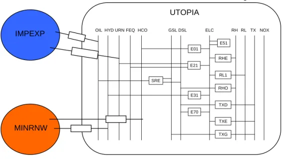
A TIMES model is structured by regions (all_r). One can distinguish between external regions and internal regions. The internal regions (r) correspond to regions within the area of study, and for which an RES has been defined by the user. Each internal region may contain processes and commodities to depict an energy system, whereas external regions serve only as origins of commodities (e.g. for import of primary energy resources or for the import of energy carriers) or as destination for the export of commodities. A region is defined as an internal region by putting it in the internal region set (r), which is a subset of the set of all regions all_r. An external region needs no explicit definition, all regions that are member of the set all_r but not member of r are external regions. A TIMES model must consist of at least one internal region, the number of external regions is arbitrary. The main building blocks of the RES are processes (p) and commodities (c), which are connected by commodity flows to form a network. An example of an RES with one internal region (UTOPIA) and two external regions (IMPEXP, MINRNW) is given in Figure 1.
All components of the energy system, as well as nearly the entire input information, are identified by a region index. It is therefore possible to use the same process name in different regions with different numerical data (and description if desired), or even completely different commodities associated with the process.
IMPEXP
MINRNW
OILHYD URN FEQ HCO GSL DSL
SRE ELC RH RL TX NOX E51 E01 E21 E31 E70 RL1 RHO TXD TXE RHE TXG
Figure 1: Example of internal and external regions in TIMES
2.2.1.1 Processes
A process may represent an individual plant, e.g. a specific existing nuclear power plant, or a generic technology, e.g. the coal-fired IGCC technology. TIMES distinguishes three main types of processes:
• Standard processes;
• Inter-regional exchange processes, and
• Storage processes.
2.2.1.1.1 Standard processes
The so-called standard processes can be used to model the majority of the energy technologies, e.g., condensing power plants, heat plants, CHP plants, demand devices such as boilers, coal extraction processes, etc. Standard processes can be classified into the following groups:
• PRE for generic energy processes;
• PRW for material processing technologies (by weight);
• PRV for material processing technologies (by volume);
• REF for refinery processes;
• ELE for electricity generation technologies;
• HPL for heat generation technologies;
• CHP for combined heat and power plants;
• DMD for demand devices;
• DISTR for distribution systems;
The topology of a standard process is specified by the set top(r,p,c,io) of all quadruples such that the process p in region r is consuming (io = ’IN’) or producing (io = ‘OUT’) commodity c. Usually, for each entry of the topology set top a flow variable (see VAR_FLO
in Chapter 4) will be created. When the so-called reduction algorithm is activated, some flow variables may be eliminated and replaced by other variables (see PART III, chapter 4).
The activity variable (VAR_ACT) of a standard process is equal to the sum of one or several commodity flows on either the input or the output side of a process. The activity of a process is limited by the available capacity, so that the activity variable establishes a link between the installed capacity of a process and the maximum possible commodity flows entering or leaving the process during a year or a subdivision of a year. The commodity flows that define the process activity are specified by the set prc_actunt(r,p,cg,u) where the commodity index cg may be a single commodity or a user-defined commodity group. The commodity group defining the activity of a process is also called Primary Commodity Group (PCG). GSL DSL OIL Refinery SRE All commodities in PJ Activity in PJ Commodity group CG_SRE Oil Diesel Gasoline
COM_GMAP(r,cg,c) = {UTOPIA.CG_SRE.DSL, UTOPIA.CG_SRE.GSL} PRC_CG(r,p,cg) = {UTOPIA.SRE.CG_SRE} PRC_ACTUNT(r,p,cg,u) = {UTOPIA.SRE.CG_SRE.PJ} Definition of commodity group Definition of process activity
Figure 2: Example of the definition of a commodity group and of the activity of a process
User-defined commodity groups are specified by means of the set com_gmap(r,cg,c), which indicates the commodities (c) belonging to the group (cg). In order to apply a user-defined commodity group in connection with a process (not only for the definition of the process activity, but also for other purposes, e.g., in the transformation equation EQ_PTRANS) one has to assign the commodity group cg to the process by specifying the
prc_cg(r,p,cg). Thus, it is possible to use the same commodity group name for different processes.
An example for the definition of the activity of a process is shown in Figure 2. In order to define the activity of the process SRE as the sum of the two output flows of gasoline (GSL) and diesel (DSL), one has to define a commodity group called CG_SRE containing these two commodities. The name of the commodity group can be arbitrarily chosen by the modeller.
different (mtoe for the capacity and PJ for the activity), the user has to supply the conversion factor from the energy unit embedded in the capacity unit to the activity unit. This is done by specifying the parameter prc_capact(r,p). In the example prc_capact has the value 41.868.
GSL DSL OIL Refinery SRE All commodities in PJ Activity in PJ Commodity group CG_SRE Oil Diesel Gasoline PRC_CAPUNT(r,p,cg,u) = {UTOPIA.SRE.CG_SRE.MTOE} PRC_CAPACT UTOPIA,SRE= 41.868 Definition of capacity unit Conversion factor from
capacity to activity unit Capacity in mtoe/a
Figure 3: Example of the definition of the capacity unit
It might occur that the unit in which the commodity(ies) of the primary commodity group are measured, is different from the activity unit. An example is shown in Figure 4. The activity of the transport technology CAR is defined by commodity TX1, which is measured in passenger kilometres PKM. The activity of the process is, however, defined in vehicle kilometres VKM, while the capacity of the process CAR is defined as number of cars NOC.
TX1 DSL Car CAR Capacity in „# of cars“ NOC Activity in „vehicle
kilometers“ VKM Commodity unit
„Passenger kilometers“ PKM
PRC_ACTUNT(r,p,cg,u) = {UTOPIA.CAR.TX1.PKM} Definition of process activity
PRC_CAPUNT(r,p,cg,u) = {UTOPIA.CAR.TX1.NOC} Definition of capacity unit
PRC_CAPACT UTOPIA, CAR= 10000
Conversion factor from capacity to activity unit
PRC_ACTFLO UTOPIA, 2000,CAR,TX1= 1.5
Conversion factor from activity unit to commodity unit
2.2.1.1.2 Inter-regional exchange processes
Inter-regional exchange (IRE) processes are used for trading commodities between regions. They are needed for linking internal regions with external regions as well as for modelling trade between internal regions. A process is specified as an inter-regional exchange process by specifying it as a member of the set prc_map(r,’IRE’,p). If the exchange process is connecting internal regions, this set entry is required for each of the internal regions trading with region r. The topology of an inter-regional exchange process p is defined by the set
top_ire(all_reg,com,all_r,c,p) stating that the commodity com in region all_reg is exported to the region all_r (the traded commodity may have a different name c in region all_r than in region all_reg). For example the topology of the export of the commodity electricity (ELC_F) from France (FRA) to Germany (GER), where the commodity is called ELC_G via the exchange process (HV_GRID) is modelled by the top_ire entry:
top_ire(‘FRA’, ’ELC_F’, ’GER’, ’ELC_G’, ’HV_GRID’).
The first pair of region and commodity (‘FRA’,’ELC_F’) denotes the origin and the name of the traded commodity, while the second pair (‘GER’,’ELC_G’) denotes the destination. The name of the traded commodity can be different in both regions, here ‘ELC_F’ in France and ‘ELC_G in Germany, depending on the chosen commodity names in both regions. As with standard processes, the activity definition set prc_actunt(r,p,cg,u) has to be specified for an exchange process belonging to each internal region. The special features related to inter-regional exchange processes are described in subsection 2.2.3.
2.2.1.1.3 Storage processes
Storage processes are used to store a commodity either between periods or between timeslices. A process (p) is specified to be an inter-period storage (IPS) process for commodity ( c ) by including it as a member of the set prc_stgips(r,p,c). In a similar way, a process is characterised as a general timeslice storage (TSS) by inclusion in the set
prc_stgtss(r,p,c). A special case of timeslice storage is a so-called night-storage device (NST) where the commodity for charging and the one for discharging the storage are different. An example for a night storage device is an electric heating technology which is charged during the night using electricity and produces heat during the day. Including a process in the set prc_nstts(r,p,s) indicates that it is a night storage device which is charged in timeslice(s) s. More than one timeslice can be specified as charging timeslices, the non-specified timeslices are assumed to be discharging timeslices. The charging and discharging commodity of a night storage device are specified by the topology set (top). It should be noted that for inter-period storage and general timeslice storage processes the commodity entering and leaving the storage is specified by the set prc_stgips(r,p,c) and prc_stgtss(r,p,c)
respectively. Other commodity flows are not permitted in combination with these two storage types and hence the topology set top is not applicable to these storages.
As for standard processes, the flows that define the activity of a storage process are identified by providing the set prc_actunt(r,p,c) entry. In contrast to standard processes, the activity of a storage process is however interpretted as the amount of the commodity being stored in the storage process. Accordingly the capacity of a storage process describes the
device).
2.2.1.2 Commodities
As mentioned before the set of commodities ( c ) is a subset of the commodity group set (cg). A commodity in TIMES is characterised by its type, which may be an energy carrier (‘NRG’), a material (‘MAT’), an emission --or environmental impact (‘ENV’), a demand commodity (‘DEM’) or a financial resource (‘FIN’). The commodity type is indicated by membership in the commodity type mapping set (com_tmap(r,com_type,c)). The commodity type affects the default sense of the commodity balance equation. For NRG, ENV and DEM the commodity production is normally greater than or equal to consumption, while for MAT and FIN the default commodity balance constraint is generated as an equality. The type of the commodity balance can be modified by the user for individual commodities by means of the commodity limit set (com_lim(r,c,lim)). The unit in which a commodity is measured is indicated by the commodity unit set (com_unit(r,c,units_com)). The user should note that within the GAMS code of TIMES no unit conversion, e.g., of import prices, takes place when the commodity unit is changed from one unit to another one. Therefore, the proper handling of the units is entirely the responsibility of the user (or the user interface).
2.2.2 Definition of the time structure
2.2.2.1 Time horizon
The time horizon for which the energy system is analysed may range from one year to many decades. The time horizon is usually split into several periods which are represented by so-called milestone years (t(allyear) or milestonyr(allyear),see Figure 5). Each milestone year represents a point in time where decisions may be taken by the model, e.g. installation of new capacity or changes in the energy flows. The activity and flow variables used in TIMES may therefore be considered as average values over a period. The shortest possible duration of a period is one year. However, in order to keep the number of variables and equations at a size that can be processed by the current solution and reporting software as well as computer hardware a period usually comprises several years. The durations of the periods do not have to be equal, so that it is possible that the first period, which usually represents the past and is used to calibrate the model to historic data, has a length of one year, while the following periods may have longer durations. Thus in TIMES both the number of periods and the duration of each period are fully under user control. The beginning year of a period
B(allyear), its ending year E(allyear), its middle year M(allyear) and its duration D(allyear)
have to be specified as input parameters by the user (see Table 12 in subsection 3.1.3), except for past years where B=E=milestonyr.
To describe capacity installations that took place before the beginning of the model horizon, and still exist during the modeling horizon, TIMES uses additional years, the so-called past years (pastyear(allyear)), which identify the construction completion year of the already existing technologies. The amount of capacity that has been installed in a pastyear is specified by the parameter NCAP_PASTI(r,allyear,p), also called past investment. For a process, an arbitrary number of past investments may be specified to reflect the age structure in the existing capacity stock. The union of the sets milestonyr and pastyear is called
to the distinction between of modelyears and datayears, the definition of the model horizon, e.g., the duration and number of the periods, may be changed without having to adjust the input data to the new periods. The rules and options of the inter- and extrapolation routine are described in more detail in subection 3.1.1.
03 04 06 07 08 09 11 12 13 14 16 17 18 19 20 02 01 Model horizon 1stperiod 2ndperiod 5thperiod 05 10 15 00 99 Milestoneyears Pastyear Datayears Modelyears 3rdperiod 4thperiod
Figure 5: Definition of the time horizon and the different year types
One should note that it is possible to define past investments (NCAP_PASTI) not only for pastyears but also for milestoneyears. Since the first period(s) of a model may cover historical data, it is useful to store the already known capacity installations made during this time-span as past investments and not as a bound on new investments in the model database. If one later changes the beginning of the model horizon to a more recent year, the capacity data of the first period(s) do not have to be changed, since they are already stored as past investments. This feature therefore supports the decoupling of the datayears, for which input information is provided, and the definition of the model horizon for which the model is run, making it relatively easy to change the definition of the modeling horizon. The use of past investments for milestoneyears is also useful to identify already planned (although not yet constructed) capacity expansions in the near future11.
G_DRATE General discount rate for currency in a particular year
G_CHNGMONY Exchange rate for currency in a particular year
MULTI Parameter multiplier table with values by year
COM_CUMPRD Cumulative limit on gross production of a commodity for a
block of years
COM_CUMNET Cumulative limit on net production of a commodity for a block
of years
CM_HISTORY Climate module calibration values; not part of the standard
TIMES code, but included in the climate module extension (see chapter 7 for a description of the climate module).
2.2.2.2 Timeslices
The milestoneyears can be further divided in sub-annual timeslices in order to describe for the changing electricity load within a year which may affect the required electricity generation capacity, or other commodity flows that need to be tracked at a finer than annual resolution. Timeslices may be organised into four hierarchy levels only: ‘ANNUAL’, ‘SEASON’, ‘WEEKLY’ and ‘DAYNITE’ defined by the internal set tslvl. The level ANNUAL consists of only one member, the predefined timeslice ‘ANNUAL,’ while the other levels may include an arbitrary number of divisions. The desired timeslice levels are activated by the user providing entries in set ts_group(r,tslvl,s), where also the individual user-provided timeslices (s) are assigned to each level. An additional user input set ts_map(r,s1,s2) is needed to determine the structure of a timeslice tree, where timeslice s1 is defined as the parent node of
s2. Figure 6 illustrates a timeslice tree, in which a year is divided into four seasons consisting of working days and weekends, and each day is further divided into day and night timeslices. The name of each timeslice has to be unique in order to be used later as an index in other sets and parameters. Not all timeslice levels have to be utilized when building a timeslice tree, for example one can skip the ‘WEEKLY’ level and directly connect the seasonal timeslices with the daynite timeslices. The duration of each timeslice is expressed as a fraction of the year by the parameter G_YRFR(r,s). The user is responsible for ensuring that each lower level group sums up properly to its parent timeslice, as this is not verified by the pre-processor. The definition of a timeslice tree is region-specific. When different timeslice names and durations are used in two regions, which are connected by an exchange process, the mapping parameters IRE_CCVT(r,c,reg,com) for commodities and IRE_TSCVT(r,s,reg,ts) for timeslices have to be provided by the user to map the different timeslice definitions. When the same timeslice definitions are used, these mapping tables do not need to be specified by the user.
12
The purpose of this table is to list those parameters whose year values are independent of the input datayears associated with most of the regular parameters, and therefore should
Commodities may be tracked and process operation controlled at a particular timeslice level by using the sets com_tsl(r,c,tslvl) and prc_tsl(r,p,tslvl) respectively. Providing a commodity timeslice level determines for which timeslices the commodity balance will be generated, where the default is ‘ANNUAL’. For processes, the set prc_tsl determines the timeslice level of the activity variable. Thus, for instance, condensing power plants may be forced to operate on a seasonal level, so that the activity during a season is uniform, while hydropower production may vary between days and nights, if the ‘DAYNITE’ level is specified for hydro power plants. Instead of specifying a timeslice level, the user can also identify individual timeslices for which a commodity or a process is available by the sets
com_ts(r,c,s) and prc_ts(r,p,s) respectively. Note that when specifying individual timeslices for a specific commodity or process by means of com_ts or prc_ts they have to be on the same timeslice level.
The timeslice level of the commodity flows entering and leaving a process are determined internally by the preprocessor. The timeslice level of a flow variable equals the timeslice level of the process when the flow variable is part of the commodity group defining the activity of the process. Otherwise the timeslice level of a flow variable is set to whichever level is finer, that of the commodity or the process.
2.2.3 Multi-regional models
If a TIMES model consists of several internal regions, it is called a multi-regional model. Each of the internal regions contains a unique RES to represent the particularities of the region. As already mentioned, the regions can be connected by inter-regional exchange processes to enable trade of commodities between the regions. Two types of trade activities can be depicted in TIMES: bi-lateral trade between two regions and multilateral trade between several supply and demand regions.
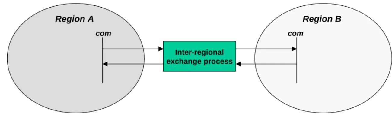
Bi-lateral trade takes place between specific pairs of regions. A pair of regions together with an exchange process and the direction of the commodity flow is first identified, where
one direction then only that direction is provided in the set top_ire (export from region r into region reg). The process capacity and the process related costs (e.g. activity costs, investment costs) of the exchange process can be described individually for both regions by specifying the corresponding parameters in each regions. If for example the investment costs for an electricity line between two regions A and B are 1000 monetary units (MU) per MW and 60 % of these investment costs should be allocated to region A and the remaining 40 % to region B, the investment costs for the exchange process have to be set to 600 MU/MW in region A and to 400 MU/MW in region B.
Inter-regional exchange process
Region A Region B
com com
Figure 7: Bilateral trade in TIMES
Bi-lateral trade is the most detailed way to specify trade between regions. However, there are cases when it is not important to fully specify the pair of trading regions. In such cases, the so-called multi-lateral trade option decreases the size of the model while preserving enough flexibility. Multi-lateral trade is based on the idea that a common marketplace exists for a traded commodity with several supplying and several consuming regions for the commodity, e.g. for crude oil or GHG emission permits. To facilitate the modelling of this kind of trade scheme the concept of marketplace has been introduced in TIMES. To model a marketplace first the user has to identify one internal region that participates both in the production and consumption of the traded commodity. Then only one exchange process is used to link the supply and demand regions with the marketplace region using the set
top_ire.13
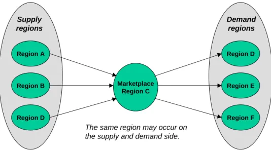
The following example illustrates the modelling of a marketplace in TIMES. Assume that we want to set up a market-based trading where the commodity CRUD can be exported by regions A, B, C, and D, and that it can be imported by regions C, D, E and F (Figure 8).
Marketplace Region C Region A Region B Region D Region D Region E Region F
The same region may occur on the supply and demand side.
Figure 8: Example of multi-lateral trade in TIMES
First, the exchange process and marketplace should be defined. For example, we could choose the region C as the marketplace region. The exchange process has the name XP. The trade possibilities can then be defined simply by the following six top_ire entries:
SET PRC / XP /; SET TOP_IRE / A .CRUD .C .CRUD .XP B .CRUD .C .CRUD .XP D .CRUD .C .CRUD .XP C .CRUD .D .CRUD .XP C .CRUD .E .CRUD .XP C .CRUD .F .CRUD .XP /;
To complete the RES definition of the exchange process, only the set prc_actunt(r,p,c,u)
is needed to define the units for the exchange process XP in all regions: SET PRC_ACTUNT / A .XP .CRUD .PJ B .XP .CRUD .PJ C .XP .CRUD .PJ D .XP .CRUD .PJ E .XP .CRUD .PJ F .XP .CRUD .PJ /;
These definitions are sufficient for setting up of the market-based trade. Additionally, the user can of course specify various other data for the exchange processes, for example investment and distribution costs, and efficiencies.
with the prefix ‘com_’ are associated with commodities, the prefix ‘prc_’ denotes process information and the prefix ‘uc_’ is reserved for sets related to user constraints. Column 3 of Table 3 is a description of each set. In some cases (especially for complex sets), two (equivalent) descriptions may be given, the first in general terms, followed by a more precise description within square brackets, given in terms of n-tuples of indices.
Remark
Set are used in basically two ways:
- as the domain over which summations must be effected in some mathematical expression, or
- as the domain over which a particular expression or constraint must be enumerated (replicated)
In the case of n-dimensional sets, some indexes may be used for enumeration and others for summation. In each such situation, the distinction between the two uses of the indexes is made clear by the way each index is used in the expression.
An example will illustrate this important point: consider the 4-dimensional set top, having indexes r,p,c,io (see table 3 for its precise description). If some quantity A(r,p,c,io) must be enumerated for all values of the third index (c=commodity) and of the last index (io=orientation), but summed over all processes (p) and regions (r), this will be mathematically denoted:
∑
∈ = top io c p r io c A r p c io EXPRESSION , , , , ( , , , ) 1It is thus understood from the indexes listed in the name of the expression (c,io), that these two indexes are being enumerated, and thus, by deduction, only r and p are being summed upon. Thus the expression calculates the total of A for each commodity c, in each direction io (‘IN’ and ‘OUT’), summed over all processes and regions.
Another example illustrates the case of nested summations, where index r is enumerated in the inner summation, but is summed upon in the outer summation. Again here, the expression is made unambiguous by observing the positions of the different indexes (for instance, the outer summation is done on the r index)
∑
∑
∈ = top io c p r p io c B r A r p EXPRESSION , , , , ( ) ( , ) 2all_reg all_r Set of all regions, internal as well as external ; a region is defined as internal by putting it in the internal region set (r), regions that are not member of the internal region set are per definition external.
c com, com1,
com2, com3
User defined list of all commodities in all regions; subset of
cg.
cg com_grp,
cg1, cg2, cg3, cg4
User defined list of all commodities and commodity groups (see Figure 2) in all regions.
clu (p)
Set of cluster technologies in endogenous technology learning.
cluster (r,teg,prc)
Indicator that technology teg is a learning component that may be part of several technologies prc; teg is also called key component [set of triplets {r,teg,prc} such that learning component teg is part of technology prc in region r].16
com_gmap (r,cg,c)
Mapping of commodity c to user-defined commodity group
cg, including itself [set of triplets {r,cg,c} such that commodity c in in group cg in region r].
com_lim (r,c,lim)
Definition of commodity balance equation type [set of triplets {r,c,lim}such that commodity c has a balance of type lim (lim=’UP’,’LO’,’EQ’) in region r]; Default: for commodities of type NRG, DM and ENV production is greater or equal consumption, while for MAT and FIN
commodities the balance is a strict equality. com_off
(r,c,y1,y2)
Specifying that the commodity c in region r is not available between the years y1 and y2 [set of quadruplets {r,c,y1,y2} such that commodity c is unavailable from years y1 to y1 in region r] ; note that y1 may be ‘BOH’ for the first year of the first period and y2 may be ‘EOH’ for the last year of the last period.
com_peak (r,cg)
set of pairs {r,cg} such that a peaking constraint is to be generated for commodity cg in region r; note that the peaking equation can be generated for a single commodity (cg also contains single commodities c) or for a group of commodities, e.g. electricity commodities differentiated by voltage level.
14
The first row contains the set name. If the set is a one-dimensional subset of another set, the second row contains the parent set in brackets. If the set is a multi-dimensional set, the second row contains the index domain in brackets.
15
For programming reasons, alternative names (aliases) may exist for some indexes. This information is only relevant for those users who are interested in gaining an understanding of
model differentiates between three electricity commodities: electricity on high, middle and low voltage ) is to be
generated for the timeslice s; Default: all timeslices of
com_ts; note that the peaking constraint will be binding only for the timeslice with the highest load.
com_tmap (r,com_type,c)
Mapping of commodities to the main commodity types (see
com_type); [set of triplets {r,com_type,c} such that commodity c has type com_type];
com_ts (r,c,s)
Set of triplets {r,c,s}such that commodity c is available in timeslice s in region r; commodity balances will be
generated for the given timeslices; Default: all timeslices of timeslice level specified by com_tsl.
com_tsl (r,c,tslvl)
Set of triplets {r,c,tslvl} such that commodity c is modelled on the timeslice level tslvl in region r; Default: 'ANNUAL timeslice level.
com_unit (r,c,units_com)
Set of triplets {r,c,units_com} such that commodity c is expressed in unit units_com in region r.
cur User defined list of currency units.
datayear Years for which model input data are to be taken; No default.
p prc User defined list of all processes in all regions
pastyear pyr Years for which past investments are specified; pastyears have to lie before the beginning of the first period; No default.
prc_actunt (r,p,cg,units_act)
Definition of activity [Set of quadruples such that the commodity group cg is used to define the activity of the process p, with units units_act, in region r].
prc_aoff (r,p,y1,y2)
Set of quadruples {r,p,y1,y2} such that process p cannot operate (activity is zero) between the years y1 and y2 in region r; note that y1 may be ‘BOH’ for first year of first period and y2 may be ‘EOH’ for last year of last period. prc_capunt
(r,p,cg,units_cap)
Definition of capacity unit of process p [set of quadruples {r,p,cg,units_cap}such that process p uses commodity group cg and units units_cap to define its capacity in region
r]. prc_cg
(r,p,cg)
User defined commodity groups (cg) associated with a process p [set of triplets {r,p,cg} such that commodity group cg has been defined for process p in region r]; note: the same commodity group can be used for several
processes. prc_dscncap
(r,p)
Set of processes p to be modelled using the lumpy
investment formulation in region r; Default: empty set. If p
is not in this set, then any lumpy investment parameters provided for p are ignored.
y1 and y2 in region r; note that y1 may be ‘BOH’ for first year of first period and y2 may be ‘EOH’ for last year of last period.
prc_grp List of process groups, used strictly for reporting purposes; Default list of groups (defined in MAPLIST.DEF) is shown in section 2.2.1.
prc_map (r,prc_grp,p)
Grouping of processes into process groups (prc_grp) [set of triplets {r,prc_grp,p} such that process p belongs to group
prc_grp in region r]. Note: used strictly for reporting purposes.
prc_noff (r,p,y1,y2)
Set of quadruples {r,p,y1,y2} such that new capacity of process p cannot be installed between the years y1 and y2 in region r; note that y1 may be ‘BOH’ for first year of first period and y2 may be ‘EOH’ for last year of last period. prc_nstts
(r,p,s)
Set of triplets {r,p,s} such that process p is a night storage device with charging timeslices s in region r; note that for night storage devices the commodity entering and the commodity leaving the storage may be different, as defined via the set top.
prc_pkaf (all_r,p)
Set of pairs {all_r,p} such that the availability factor (ncap_af) is to be used as value for the fraction of capacity of process p that can contribute to the peaking constraints
(ncap_pkcnt), in region r. prc_pkno
(all_r,p)
Set of pairs {all_r,p}such that process p cannot be used in the peaking constraints in region r.
prc_stgips (r,p,c)
Set of triplets {r,p,c}such that process p is an inter-period storage for the commodity c in region r; note that the
commodity c entering and leaving the storage is the same, so the set top is not used for this type of process.
prc_stgtss (r,p,c)
Set of triplets {r,p,c}such that process p is a storage process between timeslices (e.g., seasonal hydro reservoir, day/night pumped storage) for commodity c in region r; note that the storage process operates for the timeslices specified by
prc_ts; the same commodity c enters and leaves the storage so the set top is not used for this type of process.
prc_ts (all_r,p,s)
prc_ts2 Set of triplets {all_r,p,s} such that process p can operate at timeslice s in region r; Default: all timeslices on the
timeslice level specified by prc_tsl.. prc_tsl
(r,p,tslvl)
Set of triplets {r,p,tsllvl} such that process p can operate at timeslice level tslvl in region r; Default: ‘ANNUAL’ timeslice level.
prc_vint (r,p)
Set of processes p that are vintaged technologies, in region r i.e. technical characteristics are tied to when the capacity was installed, not the current period; Default: process is not vintaged; note that vintaging increases the model size.
and technologies are subsets of this set.
t milestonyr,
tt
Set of representative years (middle years) for the model periods within the modelling horizon.
teg Set of technologies selected for endogenous technology learning; Subset of set p; if p not in teg, then any ETL investment parameters provided are ignored.
top (r,p,c,io)
RES topology definition indicating that commodity c enters (io=’IN’) or leaves (io=’OUT’) the process p [set of
quadruples {r,p,c,io} such that process p has a flow of commodity c with orientation io in region r].
top_ire (all_reg,com, all_r,c,p)
RES topology definition for trade between regions [Set of quintuples indicating that commodity com from region
all_reg is traded (exported) via exchange process p (where it is imported) into region all_r as commodity c]; note: the name of the traded commodity may be different in the two regions.
ts_group (all_r,tslvl,s)
Set of triplets {all_r,tslvl,s} such that timeslice s belongs to the timeslice level tslvl in region r; needed for the definition of the timeslice tree; only default is that the ‘ANNUAL’ timeslice belongs to the ‘ANNUAL’ timeslice level. ts_map
(all_r,s,ts)
Set of triplets {all_r,s,ts} such that s is an intermediate node
s of the timeslice tree (neither ‘ANNUAL’ nor the lowest level), and ts is a node directly under s in region r; the set is further extended by allowing ts = s (seefigure 1).
uc_attr (r,uc_n,side, uc_grptype, uc_name)
Set of quintuples such that the TIMES attribute specified by the uc_name (e.g., capacity, flow, etc.) will be used as coefficient for the variable identified by uc_grptype in the user constraint uc_n, for the side side (‘LHS’ or ‘RHS’) in region r; if uc_name=’GROWTH’ the user constraint represents a growth constraint.
uc_grptype Fixed internal list of the key types of variables: fixed = ‘ACT_’, ‘CAP_’, ‘COMPRD_’, ‘COMCON_’, ‘FLO_’, ‘IRE_’, ‘NCAP_’.
uc_n List of user specified unique indicators of the user constraints.
uc_name The list of indicators associated with various attributes that can be referenced in user constraints to be applied when deriving a coefficient (e.g. the flow variable may be multiplied by the attribute FLO_COST to represent
expenditure associated with said flow in a user constraint if desired): = ‘ACT_COST’, ‘ACT_BNDUP’,
‘ACT_BNDLO’, ‘ACT_BNDFX’, ‘CAP_BNDUP’, ‘CAP_BNDLO’, ‘CAP_BNDFX’, ‘GROWTH’,
‘FLO_COST’, ‘FLO_DELIV’, ‘FLO_SUB’, ‘FLO_TAX’, ‘NCAP_COST’, ‘NCAP_ITAX’, ‘NCAP_ISUB’.
these constraints do not have a region index). Note that depending on the specified regions in ur_r_sum, the summation may be done only over a subset of all model regions. For example if the model contains the regions FRA, GER, ESP and one wants to create a user constraint called GHG summing over the regions FRA and GER but not ESP, the set uc_r_sum contains has the two entries
{‘FRA’,’GHG’} and {‘GER’,’GHG’}. uc_t_each
(r,uc_n,t)
Indicator that the user constraint uc_n is to be generated for each specified period t.
uc_t_succ (r,uc_n,t)
Indicator that the user constraint uc_n is to be generated between the two successive periods t and t+1.
uc_t_sum (r,uc_n,t)
Indicator that the user constraint uc_n is to be generated summing over the periods t.
uc_ts_each (r,uc_n,s)
Indicator that the user constraint uc_n will be generated for each specified timeslice s.
uc_ts_sum (r,uc_n,s)
Indicator that the user constraint uc_n is to be generated summing over the specified timeslice s .
v modlyear Union of the sets pastyear and t corresponding to all the years (periods) of a model run.
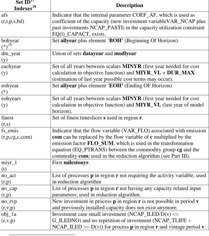
internal sets presented here concentrates on the ones frequently used in the model generator and the ones used in the description of the model equations in Chapter 5. Some internal sets are omitted from Table 5 as they are strictly auxiliary sets of the preprocessor whose main purpose is the reduction of the computation time for preprocessor operations.
Table 5: Internal sets in TIMES Set ID17
Indexes18 Description
afs
(r,t,p,s,bd)
Indicator that the internal parameter COEF_AF, which is used as coefficient of the capacity (new investment variableVAR_NCAP plus past investments NCAP_PASTI) in the capacity utilization constraint EQ(l)_CAPACT, exists.
bohyear (*)19
Set allyear plus element ‘BOH’ (Beginning Of Horizon). dm_year
(y)
Union of sets datayear and modlyear
eachyear (y)
Set of all years between scalars MINYR (first year needed for cost calculation in objective function) and MIYR_VL + DUR_MAX
(estimation of last year possible cost terms may occur). eohyear
(*)
Set allyear plus element ‘EOH’ (Ending OF Horizon) eohyears
(y)
Set of all years between scalars MINYR (first year needed for cost calculation in objective function) and MIYR_VL (last year of model horizon).
finest (r,s)
Set of finest timeslices s used in region r. fs_emis
(r,p,cg,c,com)
Indicator that the flow variable (VAR_FLO) associated with emission
com can be replaced by the flow variable of c multiplied by the emission factor FLO_SUM, which is used in the transformation equation (EQ_PTRANS) between the commodity group cg and the commodity com; used in the reduction algorithm (see Part III). miyr_1
(t)
First milestonyr. no_act
(r,p)
List of processes p in region r not requiring the activity variable; used in reduction algorithm
no_cap (r,p)
List of processes p in region r not having any capacity related input parameters; used in reduction algorithm.
no_rvp (r,v,p)
New investment in process p in region r is not possible in period v
and previously installed capacity does not exist anymore. obj_1a
(r,v,p)
Investment case small investment (NCAP_ILED/D(v) <= G_ILEDNO) and no repetition of investment (NCAP_TLIFE + NCAP_ILED >= D(v)) for process p in region r and vintage period v.
17
(r,v,p) G_ILEDNO) and repetition of investment (NCAP_TLIFE +
NCAP_ILED < D(v)) for process p in region r and vintage period v. obj_2a
(r,v,p)
Investment case large investment (NCAP_ILED/D(v) > G_ILEDNO) and no repetition of investment (NCAP_TLIFE + NCAP_ILED >= D(v)) for process p in region r and vintage period v.
obj_2b (r,v,p)
Investment case large investment (NCAP_ILED/D(v) > G_ILEDNO) and repetition of investment (NCAP_TLIFE + NCAP_ILED < D(v)) for process p in region r and vintage period v.
obj_sumi (y,r,v,p,k)
Summation control for investment and capacity related taxes and subsidies with running year index y of annual objective function, vintage period v and commissioning year k (e.g. in case of spreading investment over construction time).
obj_sumiii (y,r,v,p,k)
Summation control for decommissioning costs with for the running year index y of annual objective function, vintage period v and
commissioning year k (e.g. for spreading decommissioning costs over decommissioning time).
obj_sumiv (y,r,v,p,k)
Summation control for fixed costs with running year index y of annual objective function, vintage period v and commissioning year
k. obj_sumivs
(y,k,r,v,p)
Summation control for decommissioning surveillance costs with running year index y of annual objective function, vintage period v
and commissioning year k. obj_sums
(r,v,p)
Indicator that process p in region r with vintage period v has a salvage value for investments with a (technical) lifetime that extends past the model horizon.
obj_sums3 (r,v,p)
Indicator that process p in region r with vintage period v has a salvage value associated with the decommissioning or surveillance costs.
obj_sumsi (r,v,p,k)
Indicator that for commissioning years k process p in region r with vintage period v has a salvage value due to investment,
decommissioning or surveillance costs arsing from the technical lifetime extending past the model horizon.
periodyr (v,y)
Mapping of individual years y to the modlyear (milestonyr or
pastyear; v) period they belong to; if v is a pastyear, only the pastyear itself belongs to the period; for the last period of the model horizon also the years until the very end of the model accounting horizon (MIYR_VL + DUR_MAX) are elements of periodyr.
prc_act (r,p)
Indicator that a process p in region r needs an activity variable (used in reduction algorithm).
prc_cap (r,p)
Indicator that a process p in region r needs a capacity variable (used in reductio algorithm).