W&M ScholarWorks
W&M ScholarWorks
Undergraduate Honors Theses Theses, Dissertations, & Master Projects
4-2020
RMSE-Minimizing Confidence Intervals for the Binomial
RMSE-Minimizing Confidence Intervals for the Binomial
Parameter
Parameter
Kexin FengWilliam & Mary
Follow this and additional works at: https://scholarworks.wm.edu/honorstheses
Part of the Other Statistics and Probability Commons, Statistical Methodology Commons, Statistical Theory Commons, and the Survival Analysis Commons
Recommended Citation Recommended Citation
Feng, Kexin, "RMSE-Minimizing Confidence Intervals for the Binomial Parameter" (2020). Undergraduate Honors Theses. Paper 1456.
https://scholarworks.wm.edu/honorstheses/1456
This Honors Thesis is brought to you for free and open access by the Theses, Dissertations, & Master Projects at W&M ScholarWorks. It has been accepted for inclusion in Undergraduate Honors Theses by an authorized administrator of W&M ScholarWorks. For more information, please contact [email protected].
RMSE-Minimizing Confidence Intervals
for the Binomial Parameter
A thesis submitted in partial fulfillment of the requirement for the degree of Bachelor of Science in Mathematics from
The College of William & Mary
by Kexin Feng
Accepted for Honors
Lawrence Leemis, Director
Heather Sasinowska
Carl Moody
Williamsburg, VA May 1, 2020
Abstract
Let X1, X2, . . . , Xn be independent and identically distributed Bernoulli(p) random
variables with unknown parameter p satisfying 0 < p < 1. Let X =Pni=1Xi be the
number of successes in the n mutually independent Bernoulli trials. The maximum likelihood estimator of p is ˆp = X/n. For fixed n and α, there are n+ 1 distinct 100(1−α)% confidence intervals associated with X = 0,1,2, . . . , n. Currently there is no known exact confidence interval for p. Our goal is to construct the confidence interval for p whose actual coverage is closest to the stated coverage, using the root mean squared error, RMSE, to measure the difference between the actual coverage and the stated coverage. The approximate confidence interval for p developed here minimizes the RMSE for a sample size n and a significance levelα.
Acknowledgment
I must acknowledge my advisor and co-researcher, Professor Lawrence Leemis. More-over, I would also like to thank Professor Heather Sasinowska for supporting this research.
Contents
1 Introduction 7
2 Literature Review 9
2.1 Confidence Interval . . . 9
2.2 Actual Coverage Function . . . 12
2.3 Symmetric Dyck Path . . . 14
2.4 Conservative Confidence Intervals . . . 15
2.5 Non-Conservative Confidence Intervals . . . 19
3 Small Sample Calculations 21 3.1 One–Sample Case . . . 21
3.2 Two–Sample Case . . . 26
3.2.1 Symmetric Dyck Path 1 . . . 26
3.2.2 Symmetric Dyck Path 2 . . . 30
4 RMSE-Minimizing Confidence Interval without Smoothness 34 4.1 Interval Bound Calculations . . . 34
4.2 Dwell Time . . . 36
4.3 Epsilon-Jump . . . 37
4.4 RMSE Calculation . . . 38
4.6 Lower Bound Difference . . . 40
5 RMSE-Minimizing Confidence Interval with Smoothness 42 5.1 Smoothness . . . 42
5.2 Control for Dwell Time . . . 43
5.3 Mismatch and Rematch . . . 46
5.4 RMSE Comparison . . . 47
5.5 Asymptotic Performance . . . 50
6 Algorithm 52 6.1 Symmetric Dyck Word . . . 52
6.2 Confidence Interval Bound Calculation . . . 53
6.3 Mismatch . . . 55
7 Application 57
8 Conclusion 59
A R Code 62
B MAPLE Code 69
C RMSE-Minimizing Confidence Interval Table 72
List of Figures
2.1 Symmetric Dyck Path for n= 5. . . 15
2.2 Clopper–Pearson Confidence Interval forn = 10 and α= 0.05. . . . 17
3.1 Symmetric Dyck Path for n= 1. . . 21
3.2 The Actual Coverage Function for n= 1 and α= 0.05. . . 24
3.3 Symmetric Dyck Path for n= 2, Case 1. . . 27
3.4 The Actual Coverage Function for n= 2, α = 0.05, Case 1. . . 29
3.5 Symmetric Dyck Path for n= 2, Case 2. . . 31
3.6 The Actual Coverage Function for n= 2, α = 0.05, Case 2. . . 32
4.1 RMSE-Minimizing Confidence Intervals with no Constraints. . . 38
4.2 RMSE-Minimizing Confidence Intervals for n= 6 and α= 0.05. . . . 41
5.1 Lower Bound Difference for n= 10 and α= 0.05. . . 43
5.2 Constraints for Lower Bound Difference forn = 10 and α= 0.05. . . 45
5.3 RMSE Comparison for α= 0.05. . . 48
5.4 Smooth RMSE-Minimizing Confidence Interval forn = 10 andα= 0.05. 49 7.1 Survivor function estimate for rat survival data. . . 58
Chapter 1
Introduction
LetX1, X2, . . . , Xnbe a random sample from a Bernoulli(p) population with unknown
parameter p satisfying 0< p < 1. We develop an algorithm for constructing an ap-proximate 100(1−α)% confidence interval for p whose actual coverage is as close as possible to the stated coverage. Let X be the number of successes in then mutually independent Bernoulli trials; that is, X = Pni=1Xi. The maximum likelihood
esti-mator for p is ˆp= X/n, which is an intuitive, unbiased, and consistent estimator of
p.
Calculating interval estimators for the binomial proportion is a popular topic in statistics, with dozens of confidence interval procedures developed in the last 100 years. Applications include Monte Carlo simulation, survey sampling, and survival analysis.
All of the confidence intervals developed to date are approximate, rather than exact confidence intervals. They rely on a heuristic that results in a confidence interval forphaving an actual coverage close to the stated coverage. Our approach here differs from all previous confidence interval procedures in that we choose confidence interval bounds that optimize a measure of performance known as the root mean square error (RMSE).
It is a desirable property that the confidence interval is symmetric forX andn−X
successes. In a particular application, if we interchange the meaning of success and failure, the sets of confidence interval bounds should be symmetric about p = 0.5 because the definition of success and failure is arbitrary.
The measure of performance, RMSE, can be used to assess the effectiveness of these confidence intervals. We suggest a new non-conservative approximate confi-dence interval for p whose coverage is closer to the stated coverage than that of a constituent group of non-conservative confidence intervals: Wilson–score, Jeffreys, Agresti–Coull, and arcsine transformation. Chapter 2 contains a literature review which defines various classes of confidence intervals, plots of the actual coverage functions for these confidence interval procedures for the binomial parameter p, and formally defines of the measure of performance, RMSE. Chapter 3 concerns small sample sizes, where we manually calculate the RMSE-minimizing confidence interval bounds for n = 1 and n= 2. Chapter 4 discusses the RMSE-minimizing confidence interval without smoothness, a preferable property of the binomial confidence inter-vals. Chapter 5 introduces the “smoothness” and a set of constraints imposed on the RMSE-minimizing confidence interval to achieve smoothness. Section 6 contains an algorithm for calculating an RMSE-minimizing confidence interval and evaluates its statistical properties. Section 7 illustrates the use of the RMSE-minimizing confidence interval in an application, and Section 8 contains conclusions.
Chapter 2
Literature Review
2.1
Confidence Interval
Dekking (2005) defined a statistical confidence interval as a type of estimate computed from the observed data that reflects the precision of the associated point estimate. A confidence interval gives a range of plausible values for an unknown parameter (for example, the population mean). The interval has an associated stated coverage that the true parameter is in the proposed range. Given observations X1, X2, . . . , Xn and
a stated coverage 1−α, the probability that an exact confidence interval will contain the true underlying parameter is 1−α. The stated coverage can be chosen by the investigator. In general terms, a confidence interval for an unknown parameter is based on the sampling distribution of the corresponding point estimator.
More strictly speaking, the stated coverage represents the frequency (i.e., the proportion) of possible confidence intervals that contain the true value of the unknown population parameter. In other words, if exact confidence intervals are constructed using a given stated coverage from an infinite number of independent sample statistics, the proportion of those intervals that contain the true value of the parameter will be equal to the stated coverage (Kendall and Stuart, 1979).
For example, if the stated coverage is 0.9, then in hypothetical indefinite data collection, 90% of the samples the exact confidence interval estimates will contain the true population parameter (Illowsky, Dean, and Illowsky, 2018).
We now define these general classes of confidence intervals. Exact confidence intervals are preferred because their actual coverage equals the stated coverage. Con-fidence intervals that are not exact are approximate. Asymptotically exact conCon-fidence intervals have an actual coverage that approaches the stated coverage in the limit as the sample size n → ∞.
A random interval of the form
L < θ < U
is an exact two-sided 100(1−α)% confidence interval for the unknown parameter θ
provided
P(L < θ < U) = 1−α
for all values ofθ.
Some comments regarding exact confidence intervals are listed below.
1. The confidence interval L < θ < U is a random interval because the endpoints of the interval, L and U, are random variables that are functions of n, α, and
X1, X2, . . . , Xn. It is for this reason that the bounds are set in upper case.
2. The random variable L is known as thelower bound of the confidence interval. 3. The random variable U is known as the upper bound of the confidence interval. 4. The probability 1−α will be referred to as thestated coverage. Other terms to describe this quantity are the nominal coverage and the confidence coefficient. 5. Although α can assume any value between 0 and 1, the most common values
with these values ofα are referred to as 90%,95% and 99% confidence intervals, respectively. Because of the increased confidence, smaller values of α result in wider confidence intervals for identical data values.
A random interval of the form
L < θ < U
is anapproximate two-sided 100(1−α)% confidence interval for the unknown param-eter θ provided
P(L < θ < U)6= 1−α
for some value of θ.
A confidence interval of the form
L < θ < U
is anasymptotically exact two-sided 100(1−α)% confidence interval for the unknown parameter θ provided
lim
n→∞P(L < θ < U) = 1−α
for all values ofθ (Meeker, Hahn and Escobar, 2017).
A binomial proportion confidence interval is a confidence interval for the prob-ability of success calculated from the outcome of a series of mutually independent success–failure experiments (Bernoulli trials). In other words, a binomial proportion confidence interval is an interval estimate of the probability of success p when only the number of experiments n and the number of successesX are known.
2.2
Actual Coverage Function
The actual coveragec(p) of a confidence interval for the binomial proportion is
c(p) = n X x=0 I(x, p) n x px(1−p)n−x,
where I(x, p) is an indicator function that denotes whether a confidence interval includes the binomial proportion p when the number of successes X = x. In this thesis, we use the following terms to describe the performance, in terms of actual coverage, of a confidence interval for a binomial proportionp.
1. A confidence interval isexactif its actual coverage equals its stated (or nominal) coverage 1−α for all values of n and p, that is, c(p) = 1−α for n = 1,2, . . .
and 0< p <1.
2. A confidence interval is approximateif it is not exact. 3. A confidence interval is asymptotically exact if
lim
n→∞c(p) = 1−α
for all 0< p <1.
4. A confidence interval is conservative if c(p) ≥ 1−α for all values of n and all 0< p <1.
The defining formula for the actual coverage function c(p) and the fact that the lower bounds and upper bounds onany confidence interval procedure for the binomial proportionpare nondecreasing functions ofxmeans that the actual coverage function
c(p) must lie on one of the acceptance curves defined as
b(p, x0, x1) = x1 X x=x n x px(1−p)n−x
for a prescribed value of p, for 0 < p < 1 and for integers x0 and x1 satisfying
0 ≤ x0 ≤ x1 ≤ n. The values of p associated with the discontinuities in the actual
coverage function are the confidence interval bounds. The discontinuities in c(p) are a result of either an increase in x0 or an increase in x1 in b(p, x0, x1). If x0 is
increased, the discontinuity is associated with an upper confidence interval bound; if
x1 is increased, the discontinuity is associated with a lower confidence interval bound.
In general, there are 2n+ 1 segments in the actual coverage, which is associated with 2n+ 2 confidence interval bounds. Noticeably, there is no exact confidence interval for the binomial proportion p from a random sample of binary data values, because the actual coverage function for all confidence interval procedures must lie on one of these acceptance curves.
We now define measures for performance associated with a confidence interval for the binomial proportionp. First, the mean actual coveragemfor a confidence interval procedure is the average value of the actual coverage function for a fixed sample size
n:
m=
Z 1
0
c(p)dp.
The variance of the actual coverage v is defined as
v =
Z 1
0
c2(p)dp−m2.
The two measures of performance can be combined into a single measure by devising a calculation that is similar to the root mean squared error:
RMSE =
q
v+ m−(1−α)2,
as defined by Park and Leemis (2019). Five commonly-used confidence intervals are: Clopper–Pearson, Wilson–score, Jeffreys, Agresti–Coull, and arcsine transformation.
Our goal is to devise a confidence interval for p to minimize RMSE.
2.3
Symmetric Dyck Path
In this section, we introduce the symmetric Dyck word and the symmetric Dyck path. The one-to-one relationship between the symmetric Dyck path and the actual coverage function is a key point in our algorithm. K´asa (2010) provides a definition for a symmetric Dyck word. Let B = {0,1} be a binary alphabet, a discrete set of two symbols, and a word x1x2. . . xn ∈ Bn. Let h:B −→ {−1,1} be a valuation
function with h(0) = 1, h(1) = −1, and h(x1x2. . . xn) = Pn
i=1h(xi). A word X = x1x2x3. . . x2n ∈B2n is called a Dyck word if it satisfies the following conditions:
h(x1x2. . . xi)≥0, for i= 1,2, . . . ,2n−1 and h(x1x2. . . x2n) = 0.
A symmetric Dyck word satisfies (1−x1)(1−x2). . .(1−x2n−1)(1−x2n) = x2nx2n−1. . . x2x1.
A symmetric Dyck path is a staircase walk from (0,0) to (n, n), which lies strictly above linex1 =x0 and is symmetric with respect to linex1 =n−x0. If we associated 0
with an upward step and 1 with a rightward step, we could easily convert a symmetric Dyck word into a symmetric Dyck path. Figure 2.1 illustrates a symmetric Dyck path of length 10. It corresponds to the symmetric Dyck word 0101010101. The first entry is 0 in the Dyck word, so the first step is from (0,0) to (0,1). The second entry is 1 in the Dyck word, so the second step is from (0,1) to (1,1).
There is a one-to-one relationship between the actual coverage functions of order
n and symmetric Dyck paths of length 2n. Each discontinuity on the actual coverage is a result of an increase in either x0 or x1, and x0 ≤ x1 is required. If we plot all
(x0, x1) pairs for the actual coverage, we will get a symmetric Dyck path. Similarly,
if we can generate all the symmetric Dyck paths of length 2n, we are able to generate all the actual coverage functions of order n from them.
The number of symmetric Dyck paths of order n can be calculated by n dn/2e ,
which equalsnth central binomial coefficient (Deng, Deng, and Shapiro, 2009).
Figure 2.1: Symmetric Dyck Path for n= 5.
2.4
Conservative Confidence Intervals
In this section, we will introduce two conservative confidence intervals. Although we are not going to use these two confidence intervals when we design the RMSE-minimizing confidence interval, these two confidence intervals are widely used in prac-tice when an analyst collects n binary data values.
The Clopper–Pearson interval is usually considered to be the “gold standard” for conservative confidence intervals for p. It is based on inverting equal-tailed binomial tests of H0 : p = p0. It has endpoints that are solutions in p0 in the simultaneous equations: n X k=x n k pk0(1−p0)n−k =α/2
and x X k=0 n k pk0(1−p0)n−k=α/2,
except that the lower bound is 0 when x = 0 and the upper bound is 1 when x=n. This interval estimator is guaranteed to have coverage probability at least 1−α for every possible value of p. Whenx= 1,2, . . . , n−1, the confidence interval equals
1 + n−x+ 1 xF2x,2(n−x+1),1−α/2 −1 < p < 1 + n−x (x+ 1)F2(x+1),2(n−x),α/2 −1 ,
where Fa,b,c denotes the upper c quantile in the F distribution with a and b degrees
of freedom. A proof of this result is given in Leemis and Trivedi (1996). Equivalently, the 100(1−α)% Clopper–Pearson confidence interval for the binomial proportion p
can be expressed as the quantiles of beta distributions that is,
Bx,n−x+1,1−α/2 < p < Bx+1,n−x,α/2,
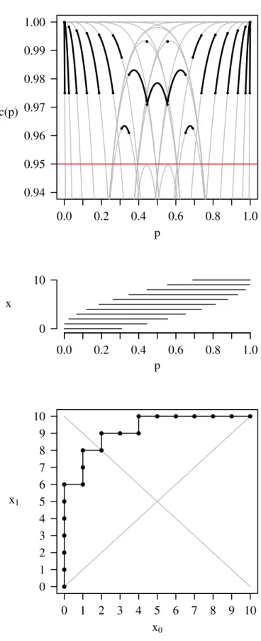
for x = 0,1,2, . . . , n, where the first two values in the subscripts are the parameters of the beta distribution and the third value in the subscript is a right-hand tail probability. Figure 2.2 contains three graphs that are associated with a sample size of n = 10 and a stated coverage of 1−α= 1−0.05 = 0.95 for the Clopper–Pearson confidence interval procedure. The top graph contains the acceptance curves in gray, the stated coverage as a red horizontal line, and the actual coverage as solid black lines. The middle graph shows then+ 1 = 11 possible confidence intervals associated with x = 0,1,2, . . . ,10. The bottom graph shows the progression of x0 and x1
0.0 0.2 0.4 0.6 0.8 1.0 0.94 0.95 0.96 0.97 0.98 0.99 1.00 p c(p) 0.0 0.2 0.4 0.6 0.8 1.0 0 10 p x 0 1 2 3 4 5 6 7 8 9 10 0 1 2 3 4 5 6 7 8 9 10 x1 x0
Notice that the confidence interval associated with x= 1, which is
0.003 < p <0.445,
has an upper bound which is quite close to the lower bound of the confidence interval associated with x= 8, which is
0.444 < p <0.975.
This is reflected in the graphs by an acceptance curve that has a very small “dwell time” (a term we will formally define in Chapter 4) of 0.001 on the top graph between
p = 0.444 and p = 0.445 on the curve that is associated with the transition from (x0, x1) = (1,7) to (x0, x1) = (1,8) to (x0, x1) = (2,8). This does not pose any
difficulty to the confidence intervals as indicated in the middle graph. The fact that the upper bound associated with x = 1 is close to the lower bound for x = 8 is coincidental. Cases will arise later in which these small dwell times do indeed cause difficulties with the confidence intervals.
Blaker (2000) has proposed a conservative confidence interval to improve the c(p) function over the Clopper–Pearson confidence interval. It is based on inverting the ex-act test with acceptance regions including the most ‘acceptable’ values of the binomial variable, where acceptability of a value x is defined by the following function
c(p) = min ( x X i=0 bn,p(i), n X j=x bn,p(j) )
where bn,p(i) and bn,p(j) denote the probability mass function of the binomial
distri-bution with parameterp. To form the acceptance region, the most ‘acceptable’ values are taken until the desired level (for example, 95%) is reached. Note that the defini-tion of the acceptability funcdefini-tion ensures that Blaker’s interval is always contained in
the Clopper–Pearson confidence interval. The Blaker confidence interval always has a smaller value of m for the associated Clopper–Pearson confidence interval for fixed values of n and α.
2.5
Non-Conservative Confidence Intervals
Four non-conservative confidence intervals will be introduced in this section. These four confidence intervals are used to control the dwell time in Chapter 5. We mainly focus on non-conservative confidence interval procedures because they result in a mean value m which is close to 1−α. By definition, a conservative confidence interval procedure results in a mean value m such that m ≥ 1−α because c(p) ≥ 1−α. The RMSE-minimizing confidence interval is going to be non-conservative due to the algorithm. Park and Leemis (2019) provides a summary of non-conservative binomial confidence intervals described next.
The bounds on the Wilson–score 100(1−α)% confidence interval for pare
1 1 +z2 α/2/2 pˆ+ z2 α/2 2n ±zα/2 s ˆ p(1−pˆ) n + z2 α/2 4n2 ,
where zα/2 is the 1−α/2 percentile of the standard normal distribution. The center
of the Wilson–score confidence interval is ˆ p+z2 α/2/(2n) 1 +z2 α/2/n ,
which is a weighted average of the point estimator ˆp=x/nand 1/2, with more weight on ˆp as n increases.
The Jeffreys 100(1−α)% confidence interval forp is a Bayesian credible interval that uses a Jeffreys noninformative prior distribution forp. As was the case with the Clopper–Pearson confidence interval, the bounds of the Jeffreys confidence interval
for pare percentiles of a beta random variable
Bx+1/2,n−x+1/2,1−α/2 < p < Bx+1/2,n−x+1/2,α/2
for x = 1,2, . . . , n−1. When x = 0, the lower bound is set to zero and the upper bound calculated using the formula above; when x = n, the upper bound is set to one and the lower bound calculated using the formula above.
The bounds of the Agresti–Coull 100(1 − α)% confidence interval, which was originally developed to approximate the Wilson-score confidence interval, are (Agresti and Coull, 1998) ˜ p±zα/2 r ˜ p(1−p˜) ˜ n , where ˜n=n+zα/2 2 and ˜p= (x+zα/2 2/2)/n˜.
The arcsine transformation uses a variance-stabilizing transformation when con-structing a confidence interval for p. Using a modification suggested by Anscombe (1956), the bounds on a 100(1−α)% confidence interval forp are
sin2 arcsinpp˜± zα/2 2√n ,
where ˜p= (x+ 3/8)/(n+ 3/4). In the rare cases in which a confidence interval does not include the point estimator, one of the bounds is adjusted to include the point estimator.
These are not the only confidence intervals for p. For example, Brown, Cai, and DasGupta (2001) gave a long list of binomial confidences intervals, including the logit interval, the likelihood ratio interval, and the Bayesian HPD interval. These intervals could have been used to control the dwell time. However, they are less frequently-used and not always recommended in literature. Therefore, we consider only the four most popular intervals described above in our confidence interval procedure.
Chapter 3
Small Sample Calculations
To better understand the actual coverage function and the intuition behind the RMSE-minimizing confidence interval, we manually calculate the optimal confidence interval bounds for n = 1 andn = 2.
3.1
One–Sample Case
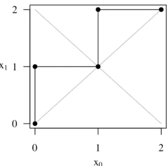
There is only one possible symmetric Dyck path for n= 1. The path starts at (0,0), moves to (0,1), and ends at (1,1). It is illustrated in Figure 3.1.
The three acceptance curves corresponding to the symmetric Dyck path are
b(p,0,0) = 1−p, b(p,0,1) = 1, b(p,1,1) =p,
for 0< p <1. Since there are two confidence intervals for n= 1, one associated with
x = 0 and the other associated with x = 1, there will be two discontinuities in the actual coverage function on 0 < p < 1. We use p1 and p2 to denote the unknown
confidence interval bounds. Since the symmetric Dyck path moves from (0,0) to (0,1) at first, p1 is associated with a lower bound. Since the symmetric Dyck path then
moves from (0,1) to (1,1), p2 is associated with an upper bound. The two confidence
intervals are 0< p < p2 for x = 0 andp1 < p <1 for x= 1. Notice that p2 = 1−p1
by symmetry. We first calculatem:
m = Z 1 0 c(p)dp = Z p1 0 (1−p)dp+ Z p2 p1 1dp+ Z 1 p2 p dp =p1− 1 2p1 2+p 2−p1+ 1 2 − 1 2p2 2 =−1 2p1 2+p 2+ 1 2− 1 2p2 2. Next we calculate v: v = Z 1 0 c2(p)dp−m2 = Z p1 0 (1−p)2dp+ Z p2 p1 12 dp+ Z 1 p2 p2dx−m2 =p1−p12+ 1 3p1 3 +p2−p1 + 1 3 − 1 3p2 3− m2 =−p12+ 1 3p1 3+p 2+ 1 3 − 1 3p2 3−m2.
Then substituting m2 = 1 4p1 4+ 1 4p2 4+ 1 2p1 2p 22−p12p2− 1 2p1 2 +1 2p2 2 −p 23+p2+ 1 4
into the expression for v results in
v = 1 3p1 3−1 2p1 2+ 1 12 + 2 3p2 3− 1 4p1 4− 1 4p2 4− 1 2p1 2p 22+p12p2− 1 2p2 2.
We arbitrarily choose α = 0.05, which results in the mean square error
RMSE2 =v + m− 19 20 2 = 1 3p1 3− 1 20p1 2+ 1 12 + 19 20 2 − 9 10p2+ 1 4 − 19 20− 1 3p2 3+ 19 20p2 2.
In order to minimize the mean square error (which also minimizes the RMSE), we take partial derivatives with respect to p1 and p2 and set equal to 0:
∂RMSE2 ∂p1 =p12− 1 10p1 = 0 ∂RMSE2 ∂p2 =− 9 10 −p2 2+19 10p2 = 0.
Solving this simultaneous set of equations for p1 and p2 results in
p1 =
1 10, p2 =
9 10.
The confidence intervals for n = 1 are displayed in Table 3.1.
L U
x= 0 0 0.9
x= 1 0.1 1
The actual coverage function is shown in Figure 3.2 by the solid lines. The three acceptance curves are shown in gray.
0.0 0.1 0.2 0.3 0.4 0.5 0.6 0.7 0.8 0.9 1.0
0.0
0.1
0.2
0.3
0.4
0.5
0.6
0.7
0.8
0.9
1.0
p
c(p)
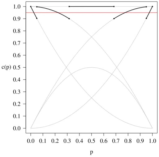
Figure 3.2: The Actual Coverage Function for n= 1 and α= 0.05.
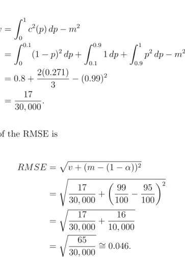
The values of m, v, and RMSE are straightforward to calculate in this case. The value ofm is m= Z 1 0 c(p)dp = Z 0.1 0 (1−p)dp+ Z 0.9 0.1 1dp+ Z 1 0.9 p dp = p− p 2 2 0.1 0 + 0.8 + p2 2 1 0.9 = 0.99.
The value ofv is v = Z 1 0 c2(p)dp−m2 = Z 0.1 0 (1−p)2dp+ Z 0.9 0.1 1dp+ Z 1 0.9 p2dp−m2 = 0.8 + 2(0.271) 3 −(0.99) 2 = 17 30,000.
Finally, the value of the RMSE is
RM SE =pv+ (m−(1−α))2 = s 17 30,000 + 99 100 − 95 100 2 = r 17 30,000 + 16 10,000 = r 65 30,000 ∼ = 0.046.
Noticeably, since the binomial confidence interval is symmetric, p2 = 1−p1 holds
in this case. In general, p2n+1−i = 1−pi always holds due to the symmetry of the
binomial confidence interval for i= 1,2, . . . ,2n.
Two observations from Table 3.2 are: (1) the RMSE-minimizing confidence in-terval procedure indeed produces the confidence inin-terval with the lowest RMSE for
p1 p2 RMSE Clopper–Pearson 0 0.025 0.975 1 0.049 Jeffreys 0 0.147 0.853 1 0.050 Wilson–score 0 0.207 0.793 1 0.064 Arcsine 0 0.012 0.988 1 0.050 Agresti–Coull 0 0.167 0.833 1 0.053 RMSE-minimizing 0 0.1 0.9 1 0.046
n= 1; and (2) the binomial confidence intervals are symmetric.
We verify the result using Maple. The code below calculates the value of p1 that
minimizes the RMSE. Becausep1 and p2 are symmetric, we set p2 = 1−p1. We have
one unknown variable p1 and one equation inp1, so we solve for the value of p1.
alpha := 1 / 20; f1 := 1 - p; f2 := 1; f3 := p; m := int(f1, p = 0 .. p1) + int(f2, p = p1 .. (1 - p1)) + int(f3, p = (1 - p1) .. 1); v := int(f1 ^ 2, p = 0 .. p1) + int(f2 ^ 2, p = p1 .. (1 - p1)) + int(f3 ^ 2, p = (1 - p1) .. 1) - m ^ 2; rmse2 := v + (m - (1 - alpha)) ^ 2; rmse2p := diff(rmse2, p1); solve(rmse2p = 0, p1);
3.2
Two–Sample Case
The situation for sample size n = 2 is more complicated. There are total of 21 = 2 symmetric Dyck paths for n= 2. We consider both cases in the two subsections that follow and compare their RMSEs.
3.2.1
Symmetric Dyck Path 1
The first symmetric Dyck path is illustrated in Figure 3.3.
Figure 3.3: Symmetric Dyck Path forn= 2, Case 1. b(p,0,0) = (1−p)2, b(p,0,1) = (1−p)2+ 2p(1−p) = 1−p2, b(p,0,2) = 1, b(p,1,2) = 2p−p2, b(p,2,2) =p2, .
for 0< p <1. There are total 2×2 + 1 = 5 segments in the actual coverage functions, which means there are 2×2 + 2 = 6 confidence interval bounds, including p= 0 and
p= 1. There are four unknown confidence interval bounds, denoted byp1, p2, p3, and p4. The three confidence intervals associated with the confidence interval bounds are
x= 0⇒0< p < p3 x= 1⇒p1 < p < p4 x= 2 ⇒p2 < p <1.
As in the previous section, we will first calculate m: m= Z 1 0 c(p) dp = Z p1 0 (1−p)2dp+ Z p2 p1 (1−p2)dp+ Z p3 p2 1 dx+ Z p4 p3 (2p−p2)dp+ Z 1 p4 p2 dp = 2 3p1 3−p 12− 1 3p2 3+p 3+p42− 2 3p4 3+1 3p3 3−p 32+ 1 3.
This time we do not calculate v. Instead, we treatv+m2 as a whole:
v+m2 = Z p1 0 (1−p)4dp+ Z p2 p1 (1−p2)2dp+ Z p3 p2 1 dp+ Z p4 p3 (2p−p2)2dp+ Z 1 p4 p4 dp =−p14+ 8 3p1 3−2p 12+ 1 5p2 5− 2 3p2 3+p 34− 1 5p3 5−4 3p3 3+p 3 + 4 3p4 3 −p 44+ 1 5.
We arbitrarily choose α = 0.05, which results in mean square error
RMSE2 =−p14+ 8 3p1 3−2p 12+ 1 5p2 5− 2 3p2 3+p 34− 1 5p3 5− 4 3p3 3+p 3+ 4 3p4 3−p 44+ 1 5− 19 15p1 3+ 19 10p1 2+19 30p2 3− 19 10p3− 19 10p4 2+19 15p4 3−19 30p3 3+19 10p3 2− 19 30.
In order to minimize the mean square error (which also minimizes the RMSE), we take partial derivatives with respect to p1, p2, p3, and p4.
∂RMSE2 ∂p1 =−p1 3+ 8p 12−4p1− 19 5 p1 2+19 5 p1 = 0 ∂RMSE2 ∂p2 =p24−2p22+ 19 10p2 2 = 0 ∂RM SE2 ∂p3 = 4p33−p34−4p32+ 1− 19 10 − 19 10p3 2+19 5 p3 = 0 ∂RMSE2 ∂p4 = 4p42−4p43+ 19 5 p4 2− 19 5 p4 = 0.
Solving this simultaneous set of equations for p1, p2, p3,and p4 results in p1 = 1 20, p2 = √ 10 10 , p3 = 1− √ 10 10 , p4 = 19 20.
Therefore, the confidence intervals forn = 2 for this particular symmetric Dyck path are displayed in Table 3.3. The actual coverage function for this case is shown in Figure 3.4.
L U
x= 0 0 0.684
x= 1 0.050 0.950
x= 2 0.316 1
Table 3.3: RMSE-Minimizing Confidence Interval Bounds for n= 2, Case 1.
0.0 0.1 0.2 0.3 0.4 0.5 0.6 0.7 0.8 0.9 1.0
0.0
0.1
0.2
0.3
0.4
0.5
0.6
0.7
0.8
0.9
1.0
p
c(p)
TheMaplecode below verifies these RMSE-minimizing values for p1, p2, p3 andp4.
These are the values of the confidence interval limits which minimize RMSE when
n= 2 and α= 0.05 for the symmetric Dyck path given in Figure 3.3.
assume(p1 > 0); assume(p1 < 1); assume(p2 > 0); assume(p2 < 1); assume(p1 < p2); alpha := 1 / 20; f1 := (1 - p) ^ 2; f2 := 1 - p ^ 2; f3 := 1; f4 := 2 * p - p ^ 2; f5 := p ^ 2; m := int(f1, p = 0 .. p1) + int(f2, p = p1 .. p2) + int(f3, p = p2 .. (1 - p2)) + int(f4, p = (1 - p2) .. (1 - p1)) + int(f5, p = (1 - p1) .. 1); v := int(f1 ^ 2, p = 0 .. p1) + int(f2 ^ 2, p = p1 .. p2) + int(f3 ^ 2, p = p2 .. (1 - p2)) + int(f4 ^ 2, p = (1 - p2) .. (1 - p1)) + int(f5 ^ 2, p = (1 - p1) .. 1) - m ^ 2; rmse2 := v + (m - (1 - alpha)) ^ 2; rmse2p1 := diff(rmse2, p1); rmse2p2 := diff(rmse2, p2);
pvalues := solve({rmse2p1 = 0, rmse2p2 = 0}, {p1, p2}); pvalue1 := pvalues[6, 1];
pvalue2 := pvalues[6, 2];
subs([p1 = pvalue1, p2 = pvalue2], m); subs([p1 = pvalue1, p2 = pvalue2], v);
subs([p1 = pvalue1, p2 = pvalue2], sqrt(rmse2));
3.2.2
Symmetric Dyck Path 2
Figure 3.5: Symmetric Dyck Path forn= 2, Case 2.
curves corresponding to this symmetric Dyck path are
b(p,0,0) = (1−p)2,
b(p,0,1) = (1−p)2+ 2p(1−p), b(p,1,1) = 2p(1−p),
b(p,1,2) = 2p−p2, b(p,2,2) = p2,
for 0< p <1. We again denote the unknown confidence interval bounds by p1, p2, p3,
andp4. The value ofp1does not change because the first two segments are the same in
these two cases. The calculation for the second confidence interval bound is unusual. If we take the partial derivative with respect to p2, that is,
∂RMSE2 ∂p2 =p2−p22+ 1 3p 3 2 = 0,
the only solution is p2 = 0, which does not satisfy 0< p2 <1.
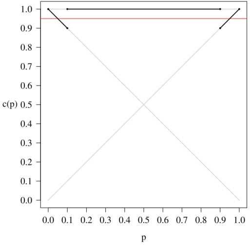
curve, which will be formally introduced in the next chapter as -jumps. Since we are unable to find a point on b(p,1,1) that minimizes the RMSE, we could stay on b(p,1,1) for only an instant, and move to b(p,1,2) immediately after b(p,0,1).
Figure 3.6 illustrates an -jump at p= 0.5.
Figures 3.4 and 3.6 indicate that symmetric Dyck path 1 results in a smaller RMSE than symmetric Dyck path 2. Table 3.4 gives the ordered confidence interval limits and RMSE values associated with n= 2 and α= 0.05.Again the RMSE-minimizing confidence interval achieves the lowest RMSE for n= 2.
0.0 0.1 0.2 0.3 0.4 0.5 0.6 0.7 0.8 0.9 1.0
0.0
0.1
0.2
0.3
0.4
0.5
0.6
0.7
0.8
0.9
1.0
p
c(p)
p1 p2 p3 p4 RMSE Clopper–Pearson 0 0.013 0.158 0.842 0.987 1 0.047 Jeffreys 0 0.061 0.333 0.667 0.939 1 0.039 Arcsine 0 0.009 0.230 0.770 0.991 1 0.044 Agresti–Coull 0 0.095 0.290 0.710 0.905 1 0.046 Wilson–score 0 0.095 0.342 0.658 0.905 1 0.046 RMSE-minimizing 0 0.050 0.316 0.684 0.950 1 0.039 Table 3.4: Confidence Interval Bounds and RMSEs for n= 2 and α= 0.05.
Forn = 3, there are total 31= 3 distinct symmetric Dyck paths. We include the MAPLE code for one of these three symmetric Dyck paths in the Appendix B.
Chapter 4
RMSE-Minimizing Confidence
Interval without Smoothness
In this chapter, we introduce the RMSE-minimizing confidence interval without smooth-ness. We derive the generalized formula and basic concepts used in constructing the RMSE-minimizing confidence interval. We compare the root mean square error of our confidence interval to those of other frequently-used non-conservative confidence intervals and conclude that the RMSE-minimizing confidence interval indeed has the lowest RMSE forn= 1,2, . . . ,12. Moreover, we notice the “smoothness,” a preferable property of the binomial confidence interval, when we calculate the confidence inter-val bounds forn = 6. We will define “smoothness” and impose a set of constraints on the RMSE-minimizing confidence interval to achieve smoothness in the next chapter.
4.1
Interval Bound Calculations
Consider the general case of an arbitrary n. When we calculate p1, we only need to
consider the terms in RMSE2 that containp
1. Letp1, p2, . . . , p2ndenote the confidence
interval bounds, andb1(p), b2(p), . . . , b2n+1(p) denote the acceptance curves associated
x1, on b for compactness and to simplify the notation. The mean square error is RMSE2 =v + (m−(1−α))2 = Z 1 0 c2(p)dp− Z 1 0 c(p) dp 2 + Z 1 0 c(p) dp−(1−α)2 2 = Z 1 0 c2(p)dp−2(1−α) Z 1 0 c(p) dp+ (1−α)2 = Z p1 0 b12(p)dp+ Z p2 p1 b22(p)dp+· · ·+ Z 1 p2n b22n+1(p) dp −2(1−α) Z p1 0 b1(p) dp+ Z p2 p1 b2(p)dp+· · ·+ Z 1 p2n b2n+1(p)dp + (1−α)2.
For all values of n, the first acceptance curve corresponds to x0 = 0 and x1 = 0,
that is, b1(p) = (1−p)n and the second acceptance curve corresponds to x0 = 0 and x1 = 1, that is, b2(p) = (1−p)n+np(1−p)n−1. In order to minimize the mean square
error (which also minimizes the RMSE), we take the partial derivative with respect top1: ∂RMSE2 ∂p1 = (1−p1)2n−(1−p1)2n−2np1(1−p1)2n−1−n2p12(1−p1)2n−2− 2(1−α)(1−p1)n+ 2(1−α)(1−p1)n+ 2(1−α)np0(1−p1)n−1 = 0 ∂RMSE2 ∂p1 =−2np1(1−p1)2n−1−n2p12(1−p1)2n−2+ 2(1−α)np1(1−p1)n−1 = 0 ∂RMSE2 ∂p1 =np1[2(1−α)(1−p1)n−1−2(1−p1)2n−1−np1(1−p1)2n−2] = 0.
We are able to achieve the value of p1 by solving
2(1−p1)n+np1(1−p1)n−1−2(1−α) = 0.
We can apply a similar calculation to any interval bound. If we hope to get the value of pc that minimizes RMSE, for c = 1,2, . . . , n, we only need to look at the
terms in RMSE2 that contain p
bc(p) and bc+1(p). Then we will take the partial derivative respect to pc and set it to
0. In this way, we derive a general formula for confidence interval bound calculation, which can be easily implemented in R.
We define the sorted 2n+2 endpoints of the confidence intervals as, 0, p1, p2, . . . , p2n,1.
The value of pc, for c = 1,2, . . . , n, which minimizes the RMSE, can be achieved by
solving 2 c−1 X x=0 n x pcx(1−pc)n−x+ n c pcc(1−pc)n−c= 2(1−α).
By symmetry,pc= 1−p2n−c+1, for c=n+ 1, n+ 2, . . . ,2n. This formula was
estab-lished generalizing the pattern associated with finding p1 given in the first paragraph
of this section.
However, this formula can be applied only when there exists a solution between 0 and 1. In many cases, we cannot find such a solution, which leads to the discussion of the dwell time and the -jump.
4.2
Dwell Time
For a particular confidence interval procedure with fixed parametersα and n, where 0 < α < 1 and n is a positive integer, we define the dwell time on an acceptance curve associated with fixed value (x0, x1) as the difference between the values of p
between two discontinuities of the actual coverage function on that acceptance curve (including p= 0 andp= 1).
For example, in the Clopper–Pearson 95% confidence interval forn = 10, the dwell time on the acceptance curve associated with (x0, x1) = (0,0) is 0.0025−0.0000 =
0.0025; on the acceptance curve associated with (x0, x1) = (0,1) is 0.0252−0.0025 =
0.0227. The longest dwell time for the Clopper–Pearson 95% confidence interval is associated with (x0, x1) = (2,8) which is 0.5549−0.4450 = 0.1099. The smallest
dwell time for the Clopper–Pearson 95% confidence interval is associated with (1,8) and (2,9), which is 0.4450−0.4439 = 0.5560−0.5549 = 0.0011. These dwell times can be seen in Figure 2.2.
4.3
Epsilon-Jump
We define an -jump to correspond to a dwell time on an acceptance curve equal to 0. One example of an -jump is the point at p = 0.5 in Figure 3.6. In that case, the actual coverage function stays on b(p,1,1) for a dwell time of length of 0. However, sometimes-jumps can cause troubles. If we allow two consecutive upwards (downwards)−jumps, confidence intervals for adjacent xmay have the same lower (upper) bounds, which is denoted as the “same bound” problem. Figure 4.1 contains the RMSE-minimizing 95% confidence intervals associated with n = 10. For these confidence intervals, the RMSE is 0.0162.As illustrated in Figure 4.1, the confidence interval for x = 5 has the same lower bound as the confidence interval for x = 6. We would strongly prefer that these two confidence intervals not have the same lower bounds. In order to achieve this criterion, we simply eliminate all the cases in which the confidence intervals for adjacentx have the same lower (upper) bounds. We will select the set of confidence intervals that has the lowest RMSE from the remaining cases. In this way, we compensate RMSE to avoid the “same bound” problem. In fact, we always need to trade off between the RMSE value and the properties of the RMSE-minimizing confidence interval. We will see more about this kind of trade-off in the latter part of this thesis.
0.0 0.1 0.2 0.3 0.4 0.5 0.6 0.7 0.8 0.9 1.0 0 1 2 3 4 5 6 7 8 9 10 p x
Figure 4.1: RMSE-Minimizing Confidence Intervals with no Constraints.
4.4
RMSE Calculation
When we achieve the confidence interval bounds for all the possible actual coverage functions, we need to calculate the RMSE for each actual coverage function, and select the actual coverage function with the lowest RMSE. Park and Leemis (2019) derive an integration-free formula for calculating the RMSE, which can effectively improve the efficiency of our algorithm.
For a fixed sample size n, a confidence interval procedure for the binomial propor-tionpassociated with x= 0,1,2, . . . , nsuccesses results inn+ 1 confidence intervals. Thus, there are 2n + 2 associated confidence interval bounds. Let p1, p2, . . . , p2n+2
denote these ordered confidence interval bounds. These bounds correspond to the endpoints of the piecewise actual coverage functionc(p). Each of the 2n+ 1 pieces of
c(p) corresponds to a piece of one of the acceptance curves
b(p, x0, x1) = x1 X x=x0 n x px(1−p)n−x.
Letx0i and x1i denote the lower and upper summation limits associated with theith
piece ofc(p), for i= 1, 2, . . . , 2n+ 1. Using this notation and the binomial theorem, an expression for the mean actual coverage which avoids numerical integration is
m = Z 1 0 c(p)dp = 2n+1 X i= 1 Z pi+1 pi x1i X x=x0i n x px(1−p)n−xdp = 2n+1 X i= 1 Z pi+1 pi x1i X x=x0i " n x px n−x X k= 0 n−x k (−p)k # dp = 2n+1 X i= 1 x1i X x=x0i Z pi+1 pi n x n−x X k= 0 n−x k (−1)kpk+xdp = 2n+1 X i= 1 x1i X x=x0i n x n−x X k= 0 n−x k (−1)k " pki+1+x+1−pki+x+1 k+x+ 1 # .
This derivation exploits the fact that the actual coverage function is a piecewise poly-nomial function in p which has a closed-form integration. Using a similar approach and again applying the binomial theorem, an expression for the variance of the actual coverage v =R01c2(p)dp−m2 which avoids numerical integration is
v = (2n+1 X i= 1 x1i X x=x0i x1i X y=x0i n x n y 2n−x−y X k= 0 2n−x−y k (−1)k " pki+1+x+y+1−pki+x+y+1 k+x+y+ 1 #) −m2.
4.5
RMSE Comparison
In this section, we compare the RMSE of the RMSE-minimizing confidence interval without smoothness with those of the Wilson–score, Jeffreys, Arcsine, and Agresti–Coull intervals for small sample sizes andα = 0.05. The RMSEs are calculated in R, which are displayed in the Table 4.1. Although we compensate a little bit RMSE to avoid the “same bound” problem, Table 4.1 shows that our confidence interval achieves the lowest RMSE, which are set in boldface type, for n = 1,2, . . . 12. Our confidence
interval is the only one that has an RMSE below 0.02 for n = 10. However, we have to acknowledge that the RMSE for n= 10 now is 0.0170 which is higher that 0.0162, the RMSE for n= 10 if we do not try to avoid the “same bound” problem.
n Wilson–score Jeffreys Arcsine Agresti–Coull RMSE-minimizing
1 0.0640 0.0500 0.0500 0.0530 0.0466 2 0.0461 0.0392 0.0440 0.0460 0.0387 3 0.0366 0.0307 0.0380 0.0378 0.0305 4 0.0326 0.0376 0.0352 0.0316 0.0261 5 0.0295 0.0268 0.0334 0.0282 0.0242 6 0.0288 0.0309 0.0333 0.0256 0.0222 7 0.0241 0.0291 0.0300 0.0250 0.0195 8 0.0244 0.0287 0.0280 0.0239 0.0213 9 0.0237 0.0277 0.0272 0.0218 0.0193 10 0.0218 0.0243 0.0260 0.0216 0.0170 11 0.0220 0.0225 0.0263 0.0215 0.0181 12 0.0213 0.0235 0.0258 0.0203 0.0167
Table 4.1: RMSE Comparison for α= 0.05.
4.6
Lower Bound Difference
In order to check whether we have successfully avoided the “same bound” problem introduced in Section 4.3, we make plots similar to Figure 4.1 for n = 1,2, . . . ,10.
We start to think about the “smoothness” when we look at the plot forn = 6, which is Figure 4.2. For x = 4, the lower bound is 0.31796649, while for x = 5, the lower bound is 0.34885285. Although confidence intervals for x = 4 and x = 5 do not share the same lower bound, their lower bound values are very close to each other as shown in Figure 4.2. We realize that simply solving the “same bound” problem is not enough. We also prefer that the differences between consecutive lower bounds are monotonically increasing. In other words, we hope the lower bound difference betweenx and x−1 is smaller than that between x+ 1 and x forx= 2,3, . . . , n−1.
this property.
Chapter 5
RMSE-Minimizing Confidence
Interval with Smoothness
In this chapter, we introduce the concept and the measure of “smoothness.” We design a set of constraints on the RMSE-minimizing confidence interval procedure to maintain smoothness. We compare the mean square error of our confidence interval to other frequently-used non-conservative confidence intervals. We conclude that our confidence interval still has a lower RMSE in most cases for n = 1,2, . . . 12.
5.1
Smoothness
In this section, we mainly focus on the “smoothness” of the binomial confidence interval. By “smoothness,” we mean that the difference between two consecutive lower bounds should get larger as x increases. For example, the difference between the lower bounds for x= 2 and x= 3 should be smaller than the difference between lower bounds for x= 3 and x = 4. Figure 5.1 plots the lower bound differences and their average of the Wilson–score, the Jeffreys, the Arcsine, and the Agresti–Coull confidence intervals forn = 10 and α= 0.05. We observe a monotonically increasing pattern.
1 2 3 4 5 6 7 8 9 10 0.00 0.05 0.10 0.15 0.20 Order of Difference Lo
wer Bound Dif
ference Wilson−Score Jeffreys Arcsine Agresti−Coull Average
Figure 5.1: Lower Bound Difference for n= 10 and α= 0.05.
We propose a new metric for smoothness. Letl0, l1, . . . , ln denote the lower bound
values for x = 0,1, . . . , n. Calculate the lower bound difference di = li − li−1 for i = 1,2, . . . , n. Calculate the ratio of two consecutive differences ri = di+1/di for i = 1,2, . . . , n−1. The smoothness index is calculated by min{r1, r2, . . . , rn−1}. If
the smoothness index is greater or equal to 1, which means the lower bound differences are non-decreasing, then we believe the confidence interval maintains the property of smoothness, or is smooth.
5.2
Control for Dwell Time
In order to avoid -jumps and preserve the smoothness, we control the dwell time on each acceptance curve by placing lower and upper bounds on the dwell time. Since this confidence interval is non-conservative, we employ four frequently-used non-conservative confidence intervals to design the dwell-time bounds. To be specific, we use the Wilson–score, Jeffreys, Arcsine, and Agresti–Coull confidence intervals
to create the dwell time bounds for lower bound differences. Since the binomial confidence interval is symmetric, the dwell time bounds will automatically control upper bound differences as well.
We create the bounds by the following steps:
1. Denote lower bounds in the RMSE-minimizing confidence interval for p associ-ated with sample size n for fixed x by l0, l1, . . . , ln. The subscripts correspond
to x, the number of observed successes. Denote the difference between two consecutive lower bounds by dk =lk−lk−1, for k = 1,2, . . . , n.
2. Generate the lower bounds for all four confidence interval procedures associated with sample size n. Denote each by lij, for i = 1,2,3,4, which indicates the
confidence interval procedure; j = 0,1, . . . , n, which indicates the number of successesx.
3. Calculate the averages of the four lower bounds ¯lj =P4i=1lij, forj = 0,1, . . . , n.
4. Calculate the lower bound difference between two consecutive lower bounds by
sk = ¯lj −¯lj−1 for k= 1,2, . . . , n.
5. We set a lower limit for each lower confidence interval bound difference as:
Lk= sk−0 2 , k = 1 sk−sk−1 2 , k= 2,3, . . . , n.
6. We set a upper limit for each lower confidence interval bound difference as:
Uk = sk+1−sk 2 , k = 1,2, . . . , n−1 1−Pni=1−1Uk, k=n.
7. We require Lk ≤dk ≤Uk, for k = 1,2, . . . , nto ensure adequate smoothness of
For example, for n= 2 and α= 0.05, the range for the first lower bound difference is (0.0323,0.149) and the range for the second lower bound difference is (0.149,0.85).
The black dots in Figure 5.2 are the averages of the lower bound differences of the Wilson–score, Jeffreys, Agresti–Coull, and Arcsine confidence intervals. The solid lines are the constraints generated from following the steps above. We could observe from Figure 5.2 that the constraints are tight in the middle and loose for xvalues at the extremes.
However, we have encountered an issue associated with the constrained lower bounds, which will be comprehensively discussed in the next section.
Order of Differences 1 2 3 4 5 6 7 8 9 10 0.00 0.05 0.10 0.15 0.20 A v erage Lo
wer Bound Dif
ference
5.3
Mismatch and Rematch
In Section 5.2, we imposed a set of constraints on the dwell time to maintain smooth-ness. However, we simultaneously created a problem, which we call “mismatch.” Mismatch refers to the situation in which the set of confidence interval bounds we get does not match the original symmetric Dyck path it corresponds to. For example, for
n = 4 and α= 0.05, one symmetric Dyck path is (0,0)→(0,1)→(0,2)→(0,3)→
(1,3) → (1,4) → (2,4)→ (3,4) → (4,4). The set of lower bounds we get with the constraints in Section 5.2 for this Dyck path is (0.00000000, 0.02501729,0.13534926,
0.30922013, 0.49952061). Due to the symmetry of the binomial confidence interval, the upper bounds are (0.5004794, 0.6907799, 0.8646507, 0.9749827, 1.0000000). The first row in Table 5.1 is the sorted lower bounds and upper bounded. The second row indicates whether it is a lower bound or a upper bound. We could observe that the fourth lower bound is smaller than the first upper bound. In other words, the fourth discontinuity (except p = 0) on this acceptance curve should associate with a lower bound. However, if we go back to look at the Dyck path, we notice that the fourth discontinuity happens between (0,3) and (1,3). The fourth discontinuity should as-sociate with a upper bound according to the symmetric Dyck path. Therefore, we observe a conflict between the symmetric Dyck path and the confidence interval bound values. We denote this conflict as a “mismatch.” One explanation for why mismatch occurs is that we only consider lower bounds when we design the control for the dwell time and ignore the relative positions of lower bounds and upper bounds on an actual coverage function.
Mismatch can lead to the miscalculation of RMSE. If we use the actual coverage 0.0000 0.0250 0.1353 0.3092 0.4995 0.5005 0.6908 0.8647 0.9750 1.000
L L L L L U U U U U
function associated with a wrong symmetric Dyck path, we are unable to get the true RMSE value. In order to solve the problem of mismatch, we introduce the idea of “rematch.” Rematch refers to the process in which we link the set of lower bounds back to the symmetric Dyck path with which it actually matches. For example, consider the set of confidence interval bounds in Table 5.1. Since the first four discontinuities are all associated with lower bounds, and the fifth to eighth discontinuities are all associated with upper bounds, the symmetric Dyck path it actually associates with is (0,0) → (0,1) → (0,2) → (0,3) → (0,4) → (1,4) → (2,4) → (3,4) → (4,4), which is different from the original symmetric Dyck path it is assigned to. Notice that due to the one-to-one relationship between the actual coverage function and the symmetric Dyck path, one set of confidence interval bounds can only be linked to one symmetric Dyck path, which makes the solution to the mismatch problem easier. After the rematch process, we are able to get the correct RMSE value.
5.4
RMSE Comparison
In this section, we compare the RMSE of our confidence interval with those of the Wilson–score, Jeffreys, Arcsine, and Agresti–Coull intervals for small sample sizes and α= 0.05. The RMSEs are calculated inR, which are displayed in Table 5.3. The lowest RMSE value for each n is set in boldface type. We observe that compared to the values in Table 4.1, RMSEs increase because of the smoothness constraints. This is a trade-off between the RMSE value and the smoothness. However, Table 5.2 and Figure 5.3 show that our confidence interval still achieves the lowest RMSE in all the cases for n = 1,2, . . . 12, except for n = 5. For n = 5, the RMSE-minimizing confi-dence interval without smoothness constraints has already achieved the smoothness, so we do not need to impose the constraints in that case. A summary of whether we should impose the smoothness constraints or not for different n will be given in the
conclusion chapter.
n Wilson–score Jeffreys Arcsine Agresti–Coull RMSE-minimizing
1 0.0640 0.0500 0.0500 0.0530 0.0466 2 0.0461 0.0392 0.0440 0.0460 0.0387 3 0.0366 0.0307 0.0380 0.0378 0.0305 4 0.0326 0.0376 0.0352 0.0316 0.0262 5 0.0295 0.0268 0.0334 0.0282 0.0269 6 0.0288 0.0309 0.0333 0.0256 0.0241 7 0.0241 0.0291 0.0300 0.0250 0.0211 8 0.0244 0.0287 0.0280 0.0239 0.0213 9 0.0237 0.0277 0.0272 0.0218 0.0207 10 0.0218 0.0243 0.0260 0.0216 0.0190 11 0.0220 0.0225 0.0263 0.0215 0.0198 12 0.0213 0.0235 0.0258 0.0203 0.0184
Table 5.2: RMSE Comparison for α= 0.05.
1 2 3 4 5 6 7 8 9 10 0.01 0.02 0.03 0.04 0.05 0.06 0.07 n RMSE Wilson−score Jeffreys Agresti−Coull Arcsine RMSE−minimizing
Figure 5.3: RMSE Comparison forα = 0.05.
0.0 0.2 0.4 0.6 0.8 1.0 0.90 0.91 0.92 0.93 0.94 0.95 0.96 0.97 0.98 0.99 1.00 p c(p) 0.0 0.2 0.4 0.6 0.8 1.0 0 10 p x 0 1 2 3 4 5 6 7 8 9 10 0 1 2 3 4 5 6 7 8 9 10 x1 x0
and a stated coverage of 1−α= 1−0.05 = 0.95 for the RMSE-minimizing confidence interval procedure with constrained dwell time. Similar to the Clopper–Pearson con-fidence interval graph in Figure 2.2, the top graph contains the acceptance curves in gray, the stated coverage as a red horizontal line, and the actual coverage as solid black lines. The middle graph shows the 11 possible confidence intervals associated withx= 0,1,2, . . . ,10. The bottom graph shows the progression ofx0 and x1
associ-ated with the jumps from one acceptance curve to another. The top graph shows that although the RMSE-minimizing confidence interval does not have an −jump, it is still possible that the dwell time on some acceptance curves is very short. The middle graph shows that no two confidence intervals for adjacent X have the same lower (or upper) bounds. If we connect the lower bounds of confidence intervals associated with eachX, we will achieve a smooth curve, which has a negative but monotonically increasing derivative. The bottom graph perfectly matches with the top graph, which means we successfully solved the problem of mismatch.
5.5
Asymptotic Performance
In practice, our algorithm could only provide results forn ≤20 because of the factorial growth in the number of Dyck paths inn. However, we could discuss the performance when n→ ∞ based on the asymptotic performances of other non-conservative bino-mial confidence intervals. Thulin (2014) pointed out that the actual coverage level may, even for large n, drop below the nominal 1−α. For example, when α = 0.05 and n= 250, the minimum actual coverage of the Jeffreys interval, the Wilson–score interval, and the Agresti–Coull interval are approximately 0.88,0.93, and 0.94 re-spectively. Neither the Jeffreys nor the Wilson–score interval has a minimum actual coverage above 0.94, even for a sample size as large asn = 2000. There is no guaran-tee that the true p is not in an unfortunate area with low coverage. However, these
coverage anomalies usually occur close to the boundaries of the parameter space. So unless we are interested in inference for pclose to 0 or 1, it may be more relevant to investigate the minimum over a central subset.
Returning to the RMSE-minimizing confidence interval, our procedure is similar to those of the Jeffreys interval, the Agresti–Coull interval, and the Wilson–score interval except that our procedure puts minimizing RMSE in the first place. Therefore, we conjecture that the RMSE-minimizing confidence interval will not be asymptotically exact. Even for n → ∞, there will exist some narrow intervals in which the actual coverage is different from the nominal coverage.
Chapter 6
Algorithm
In this chapter, we describe three algorithms used in determining the RMSE-minimizing confidence interval bounds for p. The first algorithm generates all symmetric Dyck paths, which can be converted to actual coverage functions due to the one-to-one relationship discussed in Section 2.3. The second algorithm calculates the confidence interval bounds for each actual coverage function. The third algorithm can be used to identify whether a set of confidence interval bounds matches with a symmetric Dyck path. These three algorithms help to develop our R package.
6.1
Symmetric Dyck Word
This section adapts an algorithm by K´asa (2010) to generate all symmetric Dyck paths. We use his notation as we develop our algorithm. The pseudocode given below has been implemented in R in the functiondyck given in Appendix A.
Pseudocode
Note: Indentation is used to show nesting. Parameters:
The order of symmetric Dyck word n, the number of symmetric Dyck words npt, the npt×n empty matrix DyckW ord. Procedure name: dyck
Returned value: DyckW ord
localx, i, n0, n1
x←[0,0, . . .] initialize x as a 1×n row vector
if (n0+n1 < n and n0 > n1) n0 counts the number of 0;n1 counts the number 1
i←i+ 1 i identifies the position
x[1, i]←0
n0 ←n0+ 1
dyck(x, i, n0, n1) recursive step
n0 ←n0−1
x[1, i]←1
n1 ←n1+ 1
dyck(x, i, n0, n1) recursive step
n1 ←n1+ 1
if (n0 =n1 and n0+n1 < n) i←i+ 1
x[1, i]←0
n0 ←n0+ 1
dyck(x, i, n0, n1) recursive step
n0 ←n0+ 1
if (n0+n1 =n) finish generating one Dyck path
DyckW ordrbind(DyckW ord, x) store the Dyck path in a global variable
return() end of dyck
Note: The function dyck is called recursively withindyck. The initial call: dyck(x,1,1,0)
This algorithm produces the first half of each symmetric Dyck path. The second half of each Dyck path can be easily added due to the symmetry. After generating all the symmetric Dyck paths of order n, we are able to convert them to actual coverage functions based on the one-to-one relationship.
6.2
Confidence Interval Bound Calculation
We develop a greedy algorithm to calculate the confidence interval bounds for each actual coverage function. For n≤17, the time this greedy algorithm takes is accept-able.
Pseudo Code Parameters:
The order of symmetric Dyck word n, the significance level α,
the number of symmetric Dyck words npt,
the 2npt×(2n+ 1) matrix containing all the symmetric Dyck paths, the 2×n matrix G containing the constraints for lower bound differences, the npt×(n+ 1) empty matrix LB.
Procedure type: for loop Returned value: LB
locallc, cc, f1, f2, f, po, p1, p2, pr
for (iin 1 : npt)
lc ←1 the lcth lower bound
for (j in 1 : (2n−1))
cc←DyckP ath[2i, j+ 1]−DyckP ath[2i, j]
if (cc=1) identify a lower bound
lc←lc+ 1
f1 ←f unction(p){pbinom(DyckP ath[2i, j], size=n, p)− pbinom(
DyckP ath[2i−1, j]−1, size=n, p)} current curve
f2 ←f unction(p){pbinom(DyckP ath[2i, j+ 1], size =n, p)−pbinom( DyckP ath[2i−1, j + 1]−1, size =n, p)} next curve
f ←f unction(p){f1(p) +f2(p)−2∗(1−α)} calculate the bound values po← list of solutions for f(p) = 0 without considering constraints
if (length(po)=0) no solution
p1 ←LB[i, lc−1] +G[1, lc−1] p2 ←LB[i, lc−1] +G[2, lc−1]
if (abs(f1(p1)−1 +α))> abs(f2(p1)−1 +α)){pr ←p1}
else {pr←p2} choose the one closer to the line 1−α
else if (length (po)>0) at least one solution exists for (l in 1 : length(po))
if (LB[i, lc−1] +G[1, lc−1]< po[l] and po[l]< LB[i, lc−1]+
G[2, lc−1]) if one solution satisfies the constraint
pr←po[l]
break() stop searching
else if (abs(po[1]−LB[i, lc−1]−G[1, lc−1]) < abs(po[1]
−LB[i, lc−1]−G[2, lc−1]))
pr←LB[i, lc−1] +G[1, lc−1] choose the closer constraint else {pr←LB[i, lc−1] +G[2, lc−1]} value as bound
LB[i, lc]←pr store the value
pbinom(X, n, p): CDF of binomial distribution with parameter X, n, p.
These two functions are included in the R code given in Appendix A.
The npt× (n+ 1) matrix LB contains all the lower bounds for all the actual coverage functions. We only calculate lower bounds because upper bounds can be easily calculated from lower bounds due to the symmetry of binomial confidence interval.
We do not calculate the RMSE in this function. However, the integral-free cal-culation for the RMSE in the last chapter can be easily implemented given all the confidence interval bounds.
6.3
Mismatch
In this section, we introduce a simple algorithm to identify whether a set of confidence interval bounds matches with a symmetric Dyck path. This algorithm is used to identify the mismatch problem. The rematch process can be easily developed based on this algorithm. The basic idea of this algorithm is to generate the Dyck word that the input set of confidence interval bounds corresponds to based on the order of lower and upper bounds and the Dyck word that the input Dyck path corresponds to. Then compare whether these two Dyck words are identical. If they are identical, we conclude that the set of confidence interval bounds matches the Dyck path. Pseudo Code
Parameters:
The order of symmetric Dyck word n,
the 2×(2n+ 1) matrix DP containing one symmetric Dyck path,
the 2×(n+ 1) matrix l containing a set of lower bounds in the first row and 10 in the second row,
the 2×(n+ 1) matrixu containing a set of upper bounds in the first row and 20 in the second row.
Returned value: TRUE/FALSE
bounds←cbind(l, u)
d1←c() the values in the first row for (iin 1 : 2(n+ 1))
if (bounds[2,i] == 10) identify it as a lower bounds
d1=c(d1,0) a lower bound corresponds to a 0
if (bounds[2,i] == 20) identify a upper bound, which corresponds to a 1
d1=c(d1,1) Dyck word corresponds to the interval bounds
d2←c(0)
for (iin 2 : (2∗n+ 1))
if (DyckP ath[2, i]−DyckP ath[2, i−1] == 1)
d2←c(d2,0) else d2←c(d2,1)
d2←c(d2,1) Dyck word corresponds to the input Dyck path
identical(d1, d2)
identical(x1, x2): identify whether two matrices x1 and x2 are identical. If identical,
Chapter 7
Application
The binomial confidence interval has many applications, including survival analysis and macroeconomic forecasting. This chapter adapts an example of survival analysis by Park and Leemis (2019). Consider the nonparametric estimation of the survivor function associated with the n = 7 rat survival times (in days) from Efron and Tibshirani (1993):
16 23 38 94 141 197.
The empirical survival function, which takes a downward step of 1/n = 1/7 at each data value, is given by the solid lines in Figure 7.1. The dashed lines that denote 95% confidence intervals associated with the survival probability at any time are calculated using the RMSE-minimizing 95% confidence interval. We observe that the RMSE-minimizing confidence intervals always contains the actual probabilities from the empirical function, since the solid lines always fall between the dash lines.
0 50 100 150 200 0.0 0.2 0.4 0.6 0.8 1.0 time (days) probability of surviv al
Chapter 8
Conclusion
Blyth and Still (1983) summarized four properties for approximate binomial confi-dence intervals. Let Un and Vn denote the sets of lower and upper bounds for n
mutually independent Bernoulli trials.
1. Interval-valued. It is always required that the region be an interval{Un(X), Vn(X)},
given by {Un(X)≤p≤Vn(X)}.
2. Equivariant. The problem being invariant under X →n−X and the induced
p → 1−p, it is always required that the interval be equivariant under these transformations; that is, Un(n−X) = 1−Un(X) and Vn(n−X) = 1−Vn(X).
This property is the same as the symmetry property in our thesis.
3. Monotone in x. For fixed n, it is desirable that the interval ends both be increasing in x; that is, Un(x + 1) > Un(x) and Vn(x + 1) > Vn(x). The
RMSE-minimizing confidence interval maintains this property by avoiding two consecutive lower (upper)−jumps.
4. Monotone in n. For fixed x, it is desirable that the interval ends both be de-creasing in n; that is, Un+1(x)< Un(x) andVn+1(x)< Vn(x).
We can observe that the RMSE-minimizing confidence interval without the con-straints for smoothness has already satisfied all these four requirements. Based on these four properties, we introduce a new property—smoothness—to make the RMSE-minimizing confidence interval yield more reliable estimations. However, we have to acknowledge that our constraints for smoothness increase the RMSE. There is a trade-off between the RMSE and the smoothness. Therefore, the constraints for smoothness are not necessary. Whether to use them or not depends on which one the user cares more: the RMSE or the smoothness.
Moreover, we realize that for α= 0.05, for n= 1,2, . . . ,5, the RMSE-minimizing confidence intervals achieves smoothness even if we do not impose the constraints for smoothness. In these cases, we do not need to impose the constraints since it is un-necessary for smoothness and harms the RMSE. For α= 0.05, n >5, the constraints for smoothness do not significantly increase RMSE and indeed play an important role in maintaining smoothness. Therefore, we suggest that the constraints be used for these cases. Table 8.1 shows that if we do not apply the smoothness constraints on n = 1,2, . . . ,5 and apply the smoothness constraints on n = 6,7, . . . ,12, we will achieve the lowest RMSE in all the cases for n= 1,2, . . . ,12.
n Wilson–score Jeffreys Arcsine Agresti–Coull RMSE-minimizing
1 0.0640 0.0500 0.0500 0.0530 0.0466 2 0.0461 0.0392 0.0440 0.0460 0.0387 3 0.0366 0.0307 0.0380 0.0378 0.0305 4 0.0326 0.0376 0.0352 0.0316 0.0261 5 0.0295 0.0268 0.0334 0.0282 0.0242 6 0.0288 0.0309 0.0333 0.0256 0.0241 7 0.0241 0.0291 0.0300 0.0250 0.0211 8 0.0244 0.0287 0.0280 0.0239 0.0213 9 0.0237 0.0277 0.0272 0.0218 0.0207 10 0.0218 0.0243 0.0260 0.0216 0.0190 11 0.0220 0.0225 0.0263 0.0215 0.0198 12 0.0213 0.0235 0.0258 0.0203 0.0184
In the future, we hope to develop an algorithm that allow the user to set a prefer-able smoothness, using the smoothness index we design in Section 5.1. This may require us to create more flexible constraints that are independent of other confidence intervals.
To sum up, in this thesis, we use the measure of performance for a confidence interval for a binomial proportionpdeveloped by Park and Leemis (2019): the RMSE. We construct an approximate confidence interval for pthat minimizes the RMSE for a sample size n and a significance level α. In addition, we introduce the concept of “smoothness” and add constraints on the RMSE-minimizing confidence interval to maintain “smoothness.” The RMSE-minimizing confidence interval indeed has a smaller RMSE compared to the Jeffreys, Arcsine, Agresti–Coull, and Wilson–score confidence intervals for alln = 1,2, . . . ,12.
Appendix A
R Code
This is the R code to calculate confidence interval bounds and the RMSE value for
n = 10 and α = 0.05 with smoothness constraints. The values for n and α can be arbitrarily set by the user.
#
# Clean the environment # rm(list = ls()) # # Packages used: # # install.packages("conf") # library(conf) # # install.packages("rootSolve") # library(rootSolve) #
# Important data structures # G: range for lower bounds # DyckPath: all the Dyck Paths # Finalist: all the bounds #