Reservoir characterization and modeling of lateral heterogeneity using multivariate analysis

(1)

Reservoir characterization and modeling of lateral

heterogeneity using multivariate analysis

Oluwatosin J. Rotimi1,2*_{, Bankole D. Ako}3_{, Zhenli Wang}2 1_{Petroleum Engineering Department, Covenant University, Ota, Nigeria} 2_{Key Laboratory of Petroleum Resources, Institute of Geology and Geophysics, CAS,}

Beijing 100029, China

3_{Department of Applied Geophysics, Federal University of Technology, Akure, Nigeria}

*Corresponding author. E-mail: oluwatosin.rotimi@covenantuniversity.edu.ng, tossynrotimmy@yahoo.com

(Received 11 May 2013; accepted 15 December 2013)

Abstract

Reservoir characterization deals with the description of the reservoir in detail for rock and fluid properties within a zone of interest. The scope of this study is to model lateral continuity of lithofacies and characterize reservoir rock properties using geostatistical approach on multiple data sets obtained from a structural depression in the bight of Bohai basin, China. Analytical methods used include basic log analysis with normalization. Alternating deflections observed on spontaneous potential (SP) log and resistivity log served as the basis for delineating reservoir sand units and later tied to seismic data. Computation of variogram was done on the generated petrophysical logs prior to adopting suitable simulation algorithms for the data types. Sequential indicator simulation (SIS) was used for facies modeling while sequential gaussian simulation (SGS) was adopted for the continuous logs. The geomodel built with faults and stratigraphical attitude gave unique result for the depositional environment studied. Heterogeneity was observed within the zone both in the faulted and unfaulted area. Reservoir rock properties observed follows the interfingering pattern of rock units and is either truncated by structural discontinuities or naturally pinches out. Petrophysical property models successfully accounted for lithofacies distribution. Porosity volume computed against SP volume resulted in Net to gross volume while Impedance volume results gave credibility to the earlier defined locations of lithofacies (sand and shale) characterized by porosity and permeability. Use of multiple variables in modeling lithofacies and characterizing reservoir units for rock properties has been revisited with success using hydrocarbon exploration data. An integrated approach to subsurface lithological units and hydrocarbon potential assessment has been given priority using stochastic means of laterally populating rock column with properties. This method finds application in production assessment and predicting rock properties with scale disparity during hydrocarbon exploration.

Keywords: Reservoir, Simulation, Lithofacies, Porosity, Heterogeneity, Discontinuities, Geostatistics

(2)

1. INTRODUCTION

The desire of any exploration program is to limit the number of wild cat wells drilled and optimize the siting of production wells on the oil field. This desire necessitates the need to gather much information from exploration wells that will be sufficient to base a drilling decision upon. Traditionally, the concept of well logs is to take readings of various rock properties along the bore-hole environment. Thus the various logging tools were formed to respond to these properties either in conformity with the physical theory or as an inverse function of it. To make a good deduction that relates to reservoir occurrence and fluid properties, composite well logs are required. Logs such as Gamma-ray, Spontaneous Potential, caliper, deep, medium and shallow resistivity measurements, porosity logs such as neutron, formation density and acoustic logs are all very important (Kearey et al., 2004). They are interpreted and their results integrated to arrive at a certain level of confidence which could inform of the inherent character of the reservoir of interest. This, if properly done is a huge success but it is spatially limited in resolution. Hence, the need to look at another data point that is spatially robust in as much as the cost of drilling a well is capital intensive and exploration moves to the deeper offshore environment.

Here the 3D seismic survey comes to the rescue as it proffers a solution to the challenge of areal coverage of an oil field (James et al., 1994). The sensitivity of seismic velocities to critical reservoir petrophysical parameters, such as porosity, lithofacies, pore fluid type, saturation, and pore pressure, has been recognized over the years. But the need to evaluate relational transforms between rock fluid properties and seismic responses has come to the fore as the interest of researchers. Post-depositional changes such as diagenesis and cementation often affect the outlook of sediments which may be seen on a blanket scale on seismic data. But well control tells more due to its proximity to the studied rocks (Wold et al., 2008).

Because hard data at the correct scale are scarce (due to the expense), the single most important challenge in reservoir modeling is data integration (Journel, 1994). Enormous data is usually available at various scales, accuracy and reliability during basin analysis. The challenge is to collect from the variety of data sets information relevant to the final goal of the reservoir model. The information relevant to volumetrics (in situ) calculations need not be that relevant to recovery forecasting under a complex oil recovery process. The objective is not for each reservoir discipline (e.g., geology, geophysics, and engineering) to maximize its contribution to the final reservoir model, rather the challenge is for each discipline to understand the specific forecasting goal and provide only the relevant information in a usable format and with some assessment of uncertainty (Kok and Ulker, 2007). For instance, a facies distinction need not correspond to different flow units because of hydrodynamic continuity across facies due, for example, to diagenesis or microfracturing. The major contribution of geostatistics to reservoir modeling is in data integration through predictions, interpolations and extrapolations (estimates); providing a formalism to encode vital, possibly non-numerical information; combine different data accounting for uncertainty; and transfer such uncertainty into the final forecast.

Webster and Oliver (2007), affirms that exploration environment is continuous, but properties are measurable at temporal scales. At other locations, an alternative is to

528 Reservoir characterization and modeling of lateral heterogeneity

(3)

make an estimate or predict values spatially using the temporal known values. This is the principal reason for geostatistics which permits bias less estimation with quantifiable error. It allows dealing with properties that vary in ways that are far from systematic and at all spatial scales. An additional feature of the entity of interest is that at some scale the values of its properties are positively related (technically autocorrelated). Proximally located properties often have similar values, whereas distal located properties vary in value. Geostatistics quantitatively uses the intuitive knowledge of lateral variation for prediction away from control points. Although errors are unavoidable, appropriate quantification of spatial autocorrelation to scale estimates and minimizes errors. Moreover, geostatistics is also very capable of handling questions of probability of properties occurrence at locations and at certain proportions.

1.1. Location and Study area

The field of study is in the Xinglongtai-Majuanzi structure located in the middle of western sag of Liaohe depression (Liaohe oilfield), Bohai bay in the North-east of China (Fig. 1). The age of the mega structure is Achean to Recent and there are three groups defined by age; Achean, Mesozoic and Cenozoic. The Cenozoic group is a thick body of strata deposited in the Liaohe western sag and includes the Fangshenpao Formation, Shahejie Formations (4, 3, 2, 1), Dongying Formation, Guantao Formation, Minghuazhen Formation and the quaternary layers with maximum

(4)

thickness vertical up to 8000 m (Tong et al., 2008). The area is predominantly characterized by the alluvial fan deposit that rest unconformably on the underlying volcanic joined together at the toe of the sag structure. Current exploration program has seen successful recovery of hydrocarbon from the intercalated clastic turbidite deposit which hosts the heavy hydrocarbon typical of the area. Geostatistics, 4D seismic and enhanced oil recovery methods has been adopted lately to unravel the present subsurface condition as oil is been recovered continually. The main objective of this is to prove the continuity of rock units with specific reservoir properties and remaining hydrocarbon occurrences and for its recovery. The conceptual approach of geostatistics simulation in modeling lateral occurrences of lithofacies and rock properties has been explored and the result used for dynamic reservoir simulation.

2. METHODOLOGY 2.1. Well logs workflow

Initial well logs assessment includes primary treatments and conditioning with normalization, conventional well logs analysis (Vsh, phi, K, Rw, Saturations), clustering analysis for facies prediction, fuzzy logic for missing logs predictions (Neutron), computations of essential logs for geostatistical simulation (φ, K, Sw, Shc, σ, AI, EI10,20,30, LMR, P-vel, S-vel, Vp/Vs ratio).

A centrally located well on the field has core records and additional logs of bulk density and neutron. This well served as the control used as input in the logs prediction aspect of this workflow for the missing logs. The first step was to observe the SP logs for left deflections and a corresponding right deflection log signature on LLD that translate to potential sand formation (sand top). By data integration, the proficiency of the earlier picked sand tops were checked on porosity logs crossplots. The Neutron-Density porosity crossplot logic was adopted because of the sand and shale sequences worked with. For instance equation (1) is a relation used for computation of effective porosity log that assisted in deducing porosity from density porosity log. Combining the result on a crossplot panel with a Neutron porosity logs (which is sensitive to shale formation), makes it a preferred logic in accounting for inconsistencies and erroneous deductions that may emanate from using only one of the available porosity log data to substantiate the earlier reservoir formation candidate choices from lithology and resistivity logs (Hilchie, 1979; Reimer, 1985).

(1)

where φis the porosity, ρmais the rock matrix density, ρbis the bulk density (from

density log), and ρflis the fluid density (often assumed to be density of mud filtrate). 2.2. Well logs normalization

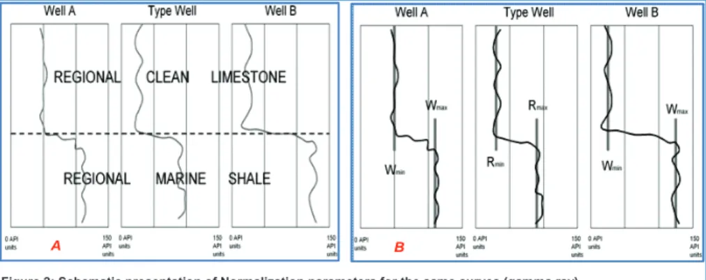
Well log normalization is the process of eliminating systematic errors from well log curves. Shier (2004), proposed improvised approaches to the classic normalization and treatment on most well logs due to acquisition challenges, natural bed configurations

φ = ρ −ρ ρ −ρ

ma b

ma fl

(5)

and fluid invasion on logging tools. Workers like Neinast and Knox (1973), Patchett and Coalson (1979), Lang (1980), Doveton and Bornemann (1981), Reimer (1985), and Shier (1997), have all contributed to the knowledge of well log normalization through histograms, crossplots and other standard techniques for comparing curve responses between well and also the use of trend surfaces for regional normalizations. Equation (2) is the general equation for a log curve whose normalized values are designated Vlog. The normalized values of the curve Vnormare given by:

(2)

Wminis the value of a specific lithology in a well. Generally Wminis near the minimum

value for that curve in that interval. Wmax is the value of a different specific

portion/lithology in each well. It is usually near the maximum value for that curve in that interval. Parameters Wmin and Wmax were taken using the uncorrected data.

Parameters Rminand Rmaxare regional best estimates of the correct value for the two

lithologies at that location, whether they are constant values or are taken from trend surfaces as reported by Doveton and Bornemann (1981). The parameters are illustrated in Figure (2). More accurate normalization results are achieved if the rock types used are picked to maximize the difference between Rmax and Rmin as is the

approach for this study.

= + − −

−

V R (R R )(V W )

(W W )

norm min

max min log min

max min

A B

Figure 2: Schematic presentation of Normalization parameters for the same curves (gamma ray). is appearance before normalization; is appearance after normalization (After Shier, 2004).B

Figure 2. Schematic presentation of Normalization parameters for the same curves (gamma ray). Ais appearance before normalization, Bis appearance after

normalization (After Shier, 2004).

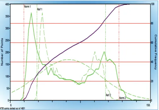
For the purpose of this study, normalization operation done was in two phases because of different aspect of the analyses. Figures 3 – 5 present a brief outlook of the procedure used. The specific curve to be normalized was viewed on the histogram through which all statistical and gaussian elements were observed and the portion/zones to be treated segmented (Fig. 3). All these was done sequel to sand top delineation. The

(6)

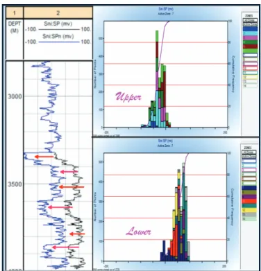
reference and normalized extent was picked and moved by 2 point method. Figure 4 are the sample histograms for the process. A is the full histogram while B and C is for upper and lower zones respectively. The curve for the lower zones was normalized to approach the uniform baselines as present on the upper zones (Fig. 5). This is clearly seen on the track 1 of Figure 5, showing the departure in the curve that has been moved from the initial baseline reference point to the eventual present point. This was done for all active wells and also at some instances in the workflow, like during the clustering run and during well log upscaling process.

2.3. Variogram analysis and simulation algorithms

This aspect of the work is usually challenging and it anchors the validity of the modeling operation for all stochastic prediction algorithms. The procedure, parameters and types of algorithms used for this aspect was based on the knowledge of the geology of the area. The procedure that initiated this was that of finding directions in data (major and minor). This is important to fixing data range(s) and search radius. This is followed by fixing tolerance angles, number of lags, radius and also bandwidth. Vertical direction was also analyzed. All these was done for every rock property with the directional modeling of major, minor and vertical axes accounting for anisotropic variogram modeling. For all directions, the degree was 40 and 85, while the variogram range was between 800 and 1500 (major and minor), 60 and 100 (vertical). Search radius was made to span the whole extent of the simulation case covering all the well locations and confined by the vertical horizon boundaries. Bandwidths were set between 4200 and 6000 (major and minor), while 30 and 50 passed for vertical

using multivariate analysis

(7)

direction. Number of lags was kept within the range 30 and 60. For geological plausibility, spherical variogram type was used with sill and nugget fixed at 1 and 0.2 respectively.

2.4. Geomodel - 3D Grid model

Single zone non-partitioned models were made for the modeled zone. The surface grid dimension 50 x 50 x 1 was chosen as most suitable after trying 100, 80 and 20 (in x and y). The model inculcates both structural and stratigraphic elements. Cell configuration (nI x nJ x nK) is 260 x 222 x 400 and total number of 3D cells is 23088000. This serves as a receptacle into which all other operations were carried out. Volumes of seismic attributes, Inversion and volume prediction results were resampled into the 3D grid model. Geostatistics analysis; variogram models and simulation algorithms were all run on the geomodel built for the zone.

All the 3D models (porosity, saturation, permeability, acoustic and elastic impedances, and facies e.t.c.) were built in a similar manner with the main difference being the type of log used to populate the grid cells, the computation formulae and simulation algorithm. Establishing the size of the model domain was critical in deciding which wells to use in the models. There was need to establish the size of the model domain. If too large an area was chosen, then there would be more space in Figure 4. Histograms used for normalization showing full log in A and upper and

(8)

between each well and less data control from the well logs. This could possibly correlate to less accurate models. Thus a reasonable zone model boundary was made to enclose the zone of interest. However, an area measuring ~144km2_{was chosen.}

The algorithms used are Kriging, Sequential Indicator Simulation (SIS), Truncated Gaussian Simulation (TGS) and Sequential Gaussian Simulation (SGS). The stochastic simulation operation starts by randomly selecting an unmeasured grid node at which a value has not yet been simulated, estimating the value and the gaussian uncertainty at the unmeasured location by kriging using the measured well data points. Furthermore, a random number is drawn from the distribution defined by the estimate and uncertainty earlier done and this simulated value assigned to the grid node. This newly simulated value is included in the set of conditioning data as though it were a real data point following which the previous steps were repeated until all measured grid nodes have a simulated value and the case is fully populated.

Figure 5. A normalization result panel showing the lower adjusted portion and respective histograms for upper and lower zones shown as B and C in figure 4

(9)

3. RESULTS AND DISCUSSION

3.1. Well logs analysis and interpretations

3.1.1. Correlation

Using logs from 12 wells, delineating hydrocarbon formations indicated divers associations of lithology types that indicate an oil-down-to (ODT) scenario for the study field (Figs. 6 and 7). The sandstone reservoir rocks are notorious for abrupt facies and porosity pinchouts with overall erratic thickness variations due to their channel sand deposition (Montgomery and Leetaru, 2000). There is virtually no clear-cut oil-water or gas-oil contact in the well logs analyzed. This then first confirms the nature of the hydrocarbon present in the reservoirs to be of heavy oil as reported by (Sircar, 2004; Yu et al.,1998; Li et al., 2008), and therefore classifying this deposit as unconventional petroleum reserve.

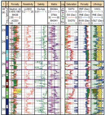
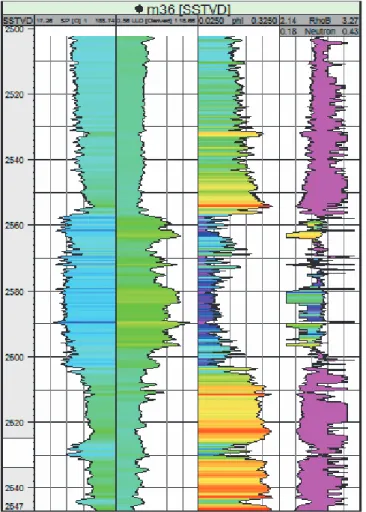
Various logs for wells m36 and m52 are presented on Figures 6 and 7 from results of conventional basic log analysis with 10 clearly labeled plot tracks each. From the left hand side to the right, track 1 has the depth values, track 2 is the main zone delineation lane, porosity log crossplot is dedicated to track 3 and on it can be seen the neutron-density crossplot logic used for the interpretations. Track 4 is dedicated to resistivity log (LLD), with a logarithmic scale of between 0.2 and 2000. Water resistivity apparent is presented on track 5 and matrix rock density property values from porosity logs (i.e. RhoMA for density matrix and DTMA for Sonic matrix) are on track 6. Track 7 is for flags of fluid occurrence. Saturation is presented on track 8

(10)

for scale of between 1 and 0. The total porosity of rock units and effective porosity computations is presented on track 9, while track 10 has the inferred lithology types and associated porosity flags.

All the potent 12 wells shows good hydrocarbon saturation flag of above 70%, while hydrocarbon is seen to be present in high percentages in portions interpreted to be higher in sand units (track 10). It is noted that clean formations are not quite present on all logs but a good associations of sand, silt and clay mix of formations on track 10. On track 3, the crossplot with the larger balloon effect indicates portions with more of shale unit with appreciable quantity of some hydrocarbon too. In all wells, this portion is seen to be characterized by high water saturation than the adjacent portions and also the matrix density is higher here. Subzones and layers indicated are picked on observing the above stated and also after visually evaluating the significant/ massive units characterized by the crossover plots of the porosity track 3. A closer look at Figures 6 and 7 shows the obvious intercalations and consistent sandwiching of sand–shale units in the whole rock column. The presence of clay makes the resistivity plot (track 4) read low and water resistivity (Rw) is adjusted to account for the movable

hydrocarbon at this depths. The formations that are indicated as clay/shale are seen to be high in porosity and with good hydrocarbon flags also. Thus, confirming the occurrence of potential source rocks inherent with the supporting sandstone formations.

(11)

3.1.2. Stratigraphical patterns

The zone modeled is most hydrocarbon prolific within the Xinglongtai-Majuanxi sag structure. Complex bedforms and formations were observed and mapped. This was particularly noticed as gradual to rapid lateral changes in lithofacies seen in the formations and computed facies logs. The neutron-density cross-plot made in the well log analysis for hydrocarbon occurrence evaluation shows various formation associations with brief non continuous lithological units as shown in Figure 8. An extensive shale blanket deposit observed in the zone interpreted is believed belong to the associated source rock present with the sandstone reservoir. The permeability of the units is generally moderate (1.0mD-2.0mD) and thus, the oil water contact could not be preserved resulting in the heavy oil that the field is known for. A longer water residency time in association with active biodegradation was the main formation mechanism for the heavy oil in this area (Li et al., 2008). The upper portion of the field is characterized by continuous clinoforms with mostly dominant reflections indicating a period of reduced or decline in depositional activity with substrate stability.

(12)

It may also be as a result of restrictions in deposition or a period of renewed deposition as it marks a formation lying unconformably on a hiatus. There are sharp boundaries in horizontal direction defining different depositional facies (clear indication of stratigraphic traps) and few dominant structural traps. This is suggested to be as a result of the regional structural pattern of the area which made the formations overlying the basement volcanic to be rotated and assume a tilting form.

Varied content of shale (Fig. 9) noticed as alternating reflection patterns in seismic data and evident on well logs, is further validated on the clustering runs done for the facies classification. Series of little units observed made the clustering run a bit challenging as more modal classes needed to be eliminated to achieve a more technically valid cluster classes. This clearly justifies the stacking patterns of the formations that indicate medium to high energy fluvial to marine depositional environments with little time for compaction. Sediment progradation and retrogradational patterns were clearly seen more on the lithological logs than on seismic sections interpreted. These patterns appeared constantly truncated in the middle portion of the seismic section by the complex faulting comb pattern. The structurally complex sub-hill region have fairly consolidated thick wedge rock units (Fig. 9), overlying volcanic basement rocks most of them serving as reservoir rock has proven to be very rich in heavy oil being explored and produced by cyclic steam and steam flood (Yu et al., 1998). The Alluvial fan turbidite formation of the field may have experienced some level of formation damage due to the production philosophy adopted for the proven reserves.

(13)

3.1.3. Structural pattern

Structural pattern takes its’ complex imprint from the major regional structural pattern. The basin being an inland basin (intracratonic) has experienced some evolution of strike-slip tectonics; consequently this has in turn, to varying degrees impacted on the attitude of the overlying formations. This is characterized by series of extensional and compressional fault configuration. This has a close semblance with the growth faulting patterns characteristic of the Niger-Delta petroleum system, but in this case no roll-over anticlines are associated with the faults and the growth pattern has been obliterated by the sag system. Also, the normal listric faults that do not appear as fault set have collapsed crest, hence forming drapes on the adjacent units and in some instances initiating the formation of adjoining thick wedge of sediments; a common pattern in the area.

Prevailing fault orientation is northeast/southwest, dipping south-easterly and trending northwest-southeast direction. There are unique faulting orientations in different seismic facies. This is in response to the alternating deformational forces from the underlying Shuangxi hidden strike-slip fault of the volcanic basement rock and the overlying major Tanlu fault that traverses the Liaohe eastern and western sag respectively (Yao and Fang, 1981; Tong et al., 2008). Hong and Yang (1984), also presented Taian Dawa fault as the controlling fault of the Liaohe western sag, and as the western of the two sub-faults of the Tanlu fault in the Liaohe Depression (Tong et al., 2008).

The clinoforms pattern on the seismic data analyzed is characterized by highly unconsolidated and chaotic interval amidst more parallel reflections indicating under-compaction and rapid deposition. This is typical of high energy alluvial fan environment with high inclination as seen around inline 2050 and beyond. The evolutional history documented in Tong et al., (2008), has also validated this that depositional activities fluctuates in intensity, weak at the beginning but amidst some cycles of rise and fall reach its strongest level in the late Oligocene. The basin being a rift basin of the Cenozoic has evolved through two important stages of rifting in the Paleocene and a depression stage in the Neogene, thereby accounting for the thick Cenozoic strata that include the hydrocarbon rich formations studied (Tong et al., 2008). Basin/field evolution suggests a Tertiary to Recent age for the deposits.

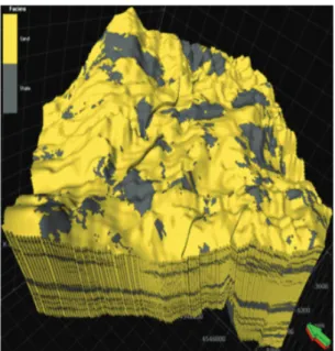
3.2. Facies model results

The Sequential indicator simulation algorithm used for the facies modeling resulted in adequate distribution of sand and shale facies taking control from the well bore axis and gently spreading its influence across according to the semi-variance/autocorrelation parameter used in the variogram modeling. Pros and cons exist with the choice of model boundary used. The non-partitioned model adopted for the simulations allowed the operations (algorithm, variogram, etc.) to assign facies values with the most freedom. No interior restraints are present to force facies assignments, so the full range of interpretation based on the variogram is displayed as all geomodel elements are also inculcated. Possible misallocated cell assignments have been adequately taken care of when the variogram model is well made. The uncertainty analysis is included in the horizon making process, thus multiple equi-probable realizations of different scenarios

(14)

of the zone properties is obtained (Fig. 10). The facies sequences are of the rapidly changing turbidite having slightly dominant lateral extensions with appreciable shale blanket. Continuity and truncations of lithological units are clearly seen on figure 11 where heterogeneity is more accentuated.

Figure 10. 15 realizations of SIS zone facies model.

(15)

3.3. Reservoir property model results

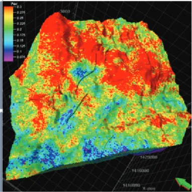
For the continuous logs up-scaled into the simulation case, the Sequential Gaussian Simulation (SGS) was used in populating the grids for reservoir properties of the zone. The variogram for each reservoir properties made with proper consideration given to the range and sill of each logs brought out facies uniqueness. This resulted from single run variogram modeling unlike the facies variogram which was done on each facies separately before carrying out a combined simulation. The orientations were also observed to be much different from that used for the facies model.

3.3.1. Porosity and Permeability model

One of the goals of the SGS model is to compare porosity model values with facies model values to discern which porosity values did not represent a sandstone facies. On observation, it was noticed that using the porosity or permeability logs alone for the purpose of facies prediction gave erroneous results and thus it was not the best option. It was seen that the greater portion of porosity property value was good as a reservoir indicator but it was also discovered to be in the range of value for shale facies thus bringing up a problem that is fundamentally of permeability. In addition, porosity and permeability modeling was subjected to co-kriging and a permeability property was used as a secondary variable when stochastically modeling a porosity model and vice versa. In the assigning of cell mean values both choices of local varying mean and collocated co-kriging were tested (Figs. 12 and 14). The approach used initializes

Figure 12. Porosity modeled with co-kriging using secondary property of permeability (local varying mean).

(16)

542 Reservoir characterization and modeling of lateral heterogeneity using multivariate analysis

Figure 13. Porosity modeled with collocated co-kriging using secondary property of permeability (constant correlation coefficient 0.7676).

Figure 14. Modeled porosity volume for zone using vertical function (i.e. regression based linear correlation cross plot of porosity and permeability).

(17)

secondary variable by treating it as a local varying mean for neighboring cells, thus stripping the interpreter of control on the net effect that the secondary variable has over the primary. The approach for the collocated co-kriging is different as an additional control parameter of correlation coefficient (0.76) is introduced between the primary and secondary variable (Fig. 13). The least square method of linear regression used in creating a vertical function that accounted for the porosity-permeability relation served as one of the variable function as input into the stochastic simulation process (Fig. 15). The correlation coefficient obtained from either a constant from each grid cell or a property may be used or a surface (i.e. a horizon with an X, Y coordinate). These proved viable in of correctly distributing the respective rock property within the simulation case as it matches with the facies distribution validation cutoff property generated with porosity and SP logs (Figs. 16 and 17). Then the log interval on the comparison log property was designated sandstone, otherwise the grid cells are populated as shale facies.

Figure 15. Porosity and permeability log property crossplot used in the Figure 14 model simulation.

(18)

Figure 16. Facies constrained SGS porosity model (i.e. facies as secondary variable).

Figure 17. SIS modeled facies used as secondary property for the porosity model in Figure 16.

(19)

Histograms of the cell value distributions of the model produced were used in evaluating the percentages of “good” and “bad” cells. In the mean of the final non-partitioned model, 86% of the cells that were designated either good or bad (disregarding the cells deemed undefined as they were able to honor prior predictions, thus termed “good”). This means 14% of the porosity model cells had porosity values less than 0.1 and also has an unassigned value within the facies distribution and SP log units. 54.34% of the overall property were designated good, 20.10% were designated bad while 25.66% got the undefined class. The cause of the bad and undefined cells may be due to the nature of the SP logs. This may be due to wash out salinity contrast via drilling mud invasion. Consequently, poorly resolved stacking patterns of the sequences used for the analysis which are quite poor in resolving bed geometry and in most cases some normalization done in short intervals. Since the grid cell assignments in each of the model is an interpretation produced by the algorithm used in populating it, the most reliable tool by which to assess the porosity and other property model’s ability to indicate sandstone facies may be the raw well logs (un-upscaled).

The sand shale formations are mostly non-continuous as it was observed also on other properties modeled, thereby confirming its heterogeneous nature and making it quite difficult to make alternative model types (such as zone partitioned model) for the area. 3.3.2. Acoustic and Elastic Impedance modeling

The most important validation for the models built in this work is its geological plausibility. This is achieved by considering the acoustic and elastic properties of the formations in the zone modeled. The result of the acoustic impedance (AI) geostatistical simulation was contrasted with the impedance volume inversion operation done on the vintage raw seismic volume (Figs. 18 and 19). There appears to be good agreement in both acoustic impedance volumes (i.e. inversion model and

(20)

stochastic model) for the zone. Although the inversion operation was exclusively deterministic and prone to the typical flaws of deterministic seismic inversion, the geostatistical approach of stochastic simulation accounted for the uncertainty thus reducing the attendant interpretation risks beyond well control. Figure 20 display the interpretation of sand units (purple pinkish-blue band on AI volume) with the density

Figure 19. SGS modeled Acoustic impedance property for the middle zone.

Figure 20. Comparison of acoustic impedance inversion output and well logs analysis for XL1355 and well 34.

(21)

log tied to the seismic section and the interpreted well logs superimposed on it. From the color band and the interpretation, it is seen and concluded that the high darker colors represent sand units while the other color band below 8000 belong to the shale facies. This was later inferred in the net to gross, histogram and cumulative distribution function made for the property.

The acoustic impedance values varies between 3000 and 17000 and from the cumulative frequency distribution curve a comparative plot gave an acceptable cut off of the impedances of the lithologies in the modeled zone (Fig. 21). Result of inversion process also agrees with this value. From the inversion operation, a cut off of 8000m/s/gcc was chosen for sand facies and below the value is the shale impedance. For optimum allocation, 50% net to gross became applicable and was plotted against the acoustic impedance value for an overall distribution.

In distinguishing the impedance contrast defined rock units, the raw and upscaled well logs resulted in admissible output with crossplots and histogram. Cut-off value (8000) inferred from the crossplot became the baseline for establishing facies limits (Fig. 22). The acoustic impedance properties of the raw logs, upscaled logs and SGS simulated result were combined and analyzed together. A cumulative distribution function was obtained that defined a peak value was used as the cut off in predicting facies from the SGS AI property model volume (Figs. 23 and 24).

(22)

Figure 22. Acoustic impedance multiple histogram and cumulative distribution function.

(23)

Figure 24. Index filtered Net to gross property derived from Acoustic impedance property using 8000m/s/gcc cutoff value.

(24)

The result of this cut-off definition from AI property gave a similar volume with the facies modeled volume. Internally on filtering the property, it was seen that all facies designated sand on original facies model were in turn designated sand with cut-off of 8000 and above, while the remaining portion of the model volume appeared with shale facies having values below 8000. This is useful in laterally tracing lithofacies by AI contrast within the zone and based on the result beyond the vicinity of the wells.

In addition to acoustic impedance stochastic simulation, Elastic impedance 10, 20 and 30degrees (EI10, EI20and EI30) computed and upscaled for simulation further assisted in laterally differentiating the rock types across the field of study. Since rock elastic property is dependent upon coefficient of rigidity, coefficient of compressibility and density variation, it became an added advantage in defining rock units. Figures 25 and 26 illustrate indexed filtered EI10and EI20property model for the interpreted zone. EI20was included in the rock property chosen in the aspect of establishing relationships over specific capture windows at different intervals within the zone. On examining simulation result of EI20, it is seen to be credible in its values with other modeled properties. EI20(far offset) engendered a plausible departure from the AI property (EI10 near offset), thereby distinguishing hydrocarbon presence in modeled lithofacies.

4. CONCLUSION

The study and modeling of rock properties utilizing well logs, seismic data and geostatistics for lateral prediction and identifying prospects beyond well control has been done. In achieving this, the various rock properties have been utilized. Consequently, 3D models were built in Petrel. These models assisted in understanding

(25)

the reservoir distribution and occurrence in the Shahejie 1 and 2 formation of Xinglongtai-majuanzi structure located in the middle of western sag of Liaohe depression (Bohai bay) in the North-east of China.

Delineation of hydrocarbon zones and fluid bearing units saw a presentation of the anomalous turbidite sequence character in the study area. Due to the thinness and rapidly changing nature of the units interpreted, the focus was on analyzing hydrocarbon for zones which has reservoir horizons as vertical boundaries. To achieve geological plausibility, the geomodel approach was used. The structural attitude and sedimentation pattern of the area was better revealed as consisting of fault echelon with series of thrust and normal fault all dipping southerly. Regional faults were rare due to the underlying geology of the Bohai bay, having both hidden and interpretable episodes of strike slip tectonics. This has conferred a wrenching effect on the strata within the basin. The variation in rock properties within the zone and across fault blocks has been clearly observed and hydrocarbon saturation values also modelled for the zone is above 70%. This is as delineated within the fault truncated fairly continuous lithological units of the zone.

This pattern prevailed all over the field but for the distal portion in the gently dipping fairly continuous wedge-like strata that rest on the regional fault. This portion serves as the site of initiation of the compressional force that seconds the regional strike slip evolutionary tectonics of the area. This compressional force and the countercurrent extensional force accounts for the structural imprints observed in the field of study.

An integrated approach to subsurface lithological units and hydrocarbon potential assessment has been given priority. This has used stochastic means to laterally populate rock column with properties. This method is useful in carrying out production assessment and predicting rock properties with scale disparity during hydrocarbon exploration.

ACKNOWLEDGEMENTS

The authors wish to appreciate Petroleum engineering subsurface research laboratory at Covenant University, TWAS-CAS postgraduate research fellowship, Liaohe oilfield for release of data and permission to publish this article and IGGCAS key laboratory of Petroleum resources.

REFERENCES

Doveton J.H. and Bornemann E., 1981. Log normalization by trend surface analysis. The Log Analyst22(4), 3-8.

Hilchie D.W., 1979. Old (pre-1958) Electrical log interpretation. Published by Hilchie D.W. Boulder, Colorado, USA, pp. 164.

Hong Z.M. and Yang Z.J., 1984. The history of generation, development and evolution of the Tancheng-Lujiang fracture in Liaoning province. Geological Bulletin of China10(3), 49-57 (in Chinese).

James H., Tellez M., Schaetzlein, G. and Stark J., 1994. Geophysical interpretation: from bits and bytes to the big picture. Oil Field Review6(3), 23-31.

(26)

Journel A.G., 1994. Stochastic Modeling and Geostatistics: Principles, Methods and Case Studies. AAPG Computer Applications in Geology3, 19-20.

Kearey P., Brooks M. and Hill I., 2004. An Introduction to Geophysical Exploration, 3rd Edition. Blackwell publishing. USA, pp. 81-82.

Kok M.V. and Ulker B., 2007. Reserve estimation using geostatistics. Energy sources, part A: recovery, utilization, and environmental effects. Taylor and Francis online30(2), 93-100.

Lang W. J., 1980. SPWLA Ad-hoc calibration committee report. The Log Analyst

21(2), 14-19.

Li S., Pang X., Liu K., Gao, X., Li X., Chen Z. and Liu B., 2008. Formation mechanism of heavy oils in the Liaohe western depression, Bohai Gulf Basin. Science in China series D: Earth Science51(2), 156-169.

Montgomery S.L. and Leetaru H.E., 2000. Storms Consolidated Field, Illinois Basin: Identifying new reserves in a mature area. American Association of Petroleum Geologists Bulletin84(2), 157-173.

Neinast G.S. and Knox C.C., 1973. Normalization of well log data. In: 14th Annual Logging Symposium Transactions. Society of Professional Well Log Analysts, 1-14. Patchett J.G. and Coalson E.B., 1979. The determination of porosity in sandstone and

shaly sandstone, Part 1-Quality control. The Log Analyst20(6), 3-12.

Reimer J.D., 1985. Density-neutron cross plot discrepancies through the Swan Hills Member, Swan Hills Unit #1, Alberta. In: Transactions of the 10th Formation Evaluation Symposium. Canadian Well Log Society (CWLS) 3, Canada, pp 15. Shier D.E., 2004. Well normalization: Methods and guidelines. Petrophysics (SPWLA)

45(3), 268-280.

Shier D.E., 1997. A comparison log response between logging companies and different vintages of tools: The Log Analyst38(3), 47–61.

Sircar A., 2004. Hydrocarbon production from fractured basement formations. Current Science87(2), 147-151.

Tong H., Fusheng Y. and Changbo G., 2008. Characteristics and Evolution of strike–slip tectonics of the Liaohe Western Sag, Bohai Bay Basin. Petroleum Science5(3), 223-229.

Webster R. and Oliver M. A., 2007. Geostatistics for Environmental Scientists, 2nd Edition. Willey-Blackwell. pp. 333.

Wold J., Grammer G.M. and Harrison W.B., 2008. Sequence Stratigraphy and 3-D Reservoir Characterization of a Silurian (Niagaran) Reef-Ray Reef Field, Macomb County, Michigan: presented at Eastern Section AAPG, Pittsburgh, PA, pp. 13-23.

Yao Y.Z. and Fang Z.J., 1981. “Tanlu Fault Colloquium” note. Seismology and Geology3(2), 69-78.

Yu L., Yang H. and Li Z., 1998. Sandstone heavy oil reservoir alteration and its influence in steam injection recovery of Liaohe oil field. Liaohe Petroleum Exploration Bureau, CNPC, Liaohe Oilfield, China. In house document, no. 1998, 128, pp. 1-7.