Open Research Online
The Open University’s repository of research publications
and other research outputs
On a class of distributions with simple exponential tails
Journal Item
How to cite:
Jones, M. C. (2008). On a class of distributions with simple exponential tails. Statistica Sinica, 18(3) pp. 1101–1110.
For guidance on citations see FAQs.
c
2008 Institute of Statistical Science, Academia Sinica Version: Accepted Manuscript
Link(s) to article on publisher’s website:
http://www3.stat.sinica.edu.tw/statistica/J18N3/J18N315/J18N315.html
Copyright and Moral Rights for the articles on this site are retained by the individual authors and/or other copyright owners. For more information on Open Research Online’s data policy on reuse of materials please consult the policies page.
On a Class of Distributions
with Simple Exponential Tails
By M.C. JONES
Department of Statistics, The Open University, Walton Hall, Milton Keynes MK7 6AA, U.K.
Summary
A simple general construction is put forward which covers many uni-modal univariate distributions with simple exponentially decaying tails (e.g. asymmetric Laplace, logF and hyperbolic distributions as well as many new models). The proposed family is a special subset of a regular exponential family, and many properties flow therefrom. Two main practical points are made in the context of maximum likelihood fitting of these distributions to data. The first of these is that three, rather than an apparent four, param-eters of the distributions suffice. The second is that maximum likelihood estimation of location in the new distributions is precisely equivalent to a standard form of kernel quantile estimation, choice of kernel being equiva-lent to specific choice of model within the class. This leads to a maximum likelihood method for bandwidth selection in kernel quantile estimation, but its practical performance is shown to be somewhat mixed. Further distribu-tion theoretical aspects are also pursued, particularly distribudistribu-tions related to the main construction as special cases, limiting cases or by simple transfor-mation.
Some key words: Asymmetric Laplace distribution; Bandwidth selection; Expo-nential family; Hyperbolic distribution; Kernel quantile estimation; Log F distri-bution; Maximum likelihood.
1. Introduction
A continuous univariate distribution onR has simple exponential tails if its density f has the properties
f(x)∼eαx asx→ −∞, f(x)∼e−βx asx→ ∞, (1) for some α, β > 0. The archetypal example of such a distribution is the asymmetric Laplace distribution given by
fAL(x) = αβ
α+β exp{αxI(x <0)−βxI(x≥0)}. (2)
For an excellent treatment of this distribution, see Kotz, Kozubowski and Podg´orski (2001, Chapter 3). It is particularly simple, its one drawback, to some, being its ‘pointed’ nature at x= 0 and its non-differentiability there.
Which other distributions share the property of simple exponential tails? I could think of two before starting this work — the log F and hyperbolic distributions — and they will feature below. (Their properties include much smoother behaviour than the asymmetric Laplace around x = 0.) The pur-pose of this paper is to present a simple general construction involving the two parametersα, β >0 which affords a wide variety of distributions with tail behaviour (1) (and of which the asymmetric Laplace, log F and hyperbolic distributions remain probably the most important). The family proposed will be a special subset of a regular exponential family.
Input to this construction will simply be one’s favourite (simple, symmet-ric) distribution which has random variableXG, densityg, distribution func-tion Gand first iterated (left-tail) distribution functionG[2](x) =−∞x G(t)dt
which isG(x) times the mean residual life function (e.g. Bassan, Denuit and Scarsini, 1999, and references therein). The latter does not exist if g(x) goes as|x|−(γ+1) for 0< γ≤1 asx→ −∞, so any such (very heavy tailed)
distri-butions — ‘Cauchy and heavier’ — are disqualified from consideration. Then,
G[2](x) =E{(x−XG)I(XG< x)}. Takingg to be symmetric (about zero) is a convenience that affords particularly elegant simplifications without losing importantly in generality and which will be followed virtually throughout this paper.
The main construction and numerous basic properties are given in Sec-tion 2. A variety of special cases are considered in SecSec-tion 3. DistribuSec-tions linked to the main construction as limiting cases are derived in Section 4. In
Sections 5 and 6, two major practical points are made in the context of max-imum likelihood fitting of the new distributions to data. The first of these (Section 5) explores whether the new construction really needs all four of its parameters in practice. The answer is negative: three parameters suffice. The second of these sections (Section 6) observes that maximum likelihood estimation of location in the new distributions is precisely equivalent to a standard form of kernel quantile estimation. (This was a major motivation for the current work: specific choice of kernel is equivalent to specific choice of model within the class.) This leads to a maximum likelihood method for bandwidth selection in kernel quantile estimation, but its practical perfor-mance is shown to be somewhat mixed. Finally, a number of distributions related to our main construction through simple transformations are explored in Section 7.
2 General construction and properties
The proposed general family of distributions with simple exponential tails has density
fG(x) =K−G1(α, β) exp{αx−(α+β)G[2](x)}. (3) It is clear that as x → −∞, G[2](x) → 0 and that — the real key to the construction — as x → ∞, G[2](x) ∼ x. That fG has simple exponential tails as at (1) is thus clear. Note that this holds regardless of the weight of the tails of allowed G.
The exponential tails also ensure integrability of fG so that the claim that it defines a density is confirmed, albeit one for which the normalisation constant KG(α, β) is not available in closed form in general. Likewise, the exponential tails imply the existence of all moments of the distribution, but their explicit formulae are also available only on a case-by-case basis. These comments are reflected in the moment generating function associated with (3) which, for −α < t < β, is immediately seen to take the form KG(α+
t, β −t)/KG(α, β). Similarly, the characteristic function is KG(α+it, β − it)/KG(α, β). DefineKijG(α, β) = ∂i+jK
G(α, β)/∂αi∂βj.Then, inter alia, the
mean of distribution (3) is {KG10(α, β)− KG01(α, β)}/KG(α, β).
Densities (3) are, immediately, unimodal for all α, β > 0 with mode x0
of G. Moreover, densities (3) are all log-concave, i.e. strongly unimodal, in
x. Let XFG follow the distribution with density fG. It is also the case that
E(G(XFG)) = α/(α+β).
For symmetric g, two apparent alternative formulations turn out to be essentially the same as (3). Let ¯G[2](x) = x∞{1− G(t)}dt = E{(XG − x)I(XG > x)} be the first iterated right-tail distribution function; it is easy to see that for symmetric g, ¯G[2](x) = G[2](−x). First, one might consider the density proportional to exp{−βx−(α+β) ¯G[2](x)} but this is just the distribution of−XFG with the roles ofα and β swopped. Second, one might consider the more symmetric formulation in which the density is proportional to
exp{−αG¯[2](x)−βG[2](x)}, (4) but this turns out to be nothing other than density (3) again. This is because, for symmetric g,
G[2](x)−G¯[2](x) =E(x−XG) =x.
Formulation (4), in particular, makes it immediately clear that fG is symmetric (about zero) if and only if α = β (for symmetric g). Indeed, in that case, symmetric densities are proportional to the α’th power of density (3) with α=β = 1.
3. Special cases
3·1. The asymmetric Laplace distribution
The asymmetric Laplace density (2) is the very special case of density (3) when G corresponds to a point mass at zero: G(x) = I(x ≥ 0), G[2](x) =
xI(x≥0).
3·2. The log F distribution
Now let G be the logistic distribution so that G(x) = ex/(1 + ex) and
G[2](x) = log(1 +ex). It follows that the resulting density
fLF(x)∝ e
αx
and it can readily be calculated thatKLF(α, β) =B(α, β) whereB(·,·) is the beta function. This is none other than the log F distribution which dates back to R.A. Fisher (as the z distribution) and which has appeared from time to time and in a variety of guises in the literature since then. For a partial review and references, see Jones (2006a).
The logistic distribution also ‘generates’ the log F distribution in the following way. The ith order statistic of an i.i.d. sample of size n from the logistic distribution follows the log F distribution with α=i, β =n+ 1−i. Moreover, in Jones (2004), I argue that replacing the integers i and n by a pair of real parameters provides a general method for generating distributions with two extra shape parameters from a simple initial distribution.
3·3. The hyperbolic distribution
Now let G be the (scaled) t2 distribution (the Student t distribution on two degrees of freedom) such that G(x) = (1/2)(1 +x/√1 +x2) and
G[2](x) = (1/2)(x+√1 +x2). The resulting density is that of the hyper-bolic distribution of Barndorff-Nielsen (1977), see also Barndorff-Nielsen and Blaesild (1983): fH(x)∝exp α−β 2 x− α+β 2 √ 1 +x2 .
It turns out that KH(α, β)= (α+β)K1(√αβ)/√αβ where K1(·) is a Bessel function. This parametrisation is not, perhaps, the most usual one which takes as parameters π = (α−β)/2√αβ and ξ = √αβ (Barndorff-Nielsen and Blaesild, 1983), but it is one of the alternative forms listed by those au-thors. Of course, consideration of logfH and its hyperbolic form makes the hyperbolic distribution an especially natural member of the class of distribu-tions with simple exponential tails from the viewpoint of linear asymptotes for the log density.
In Jones (2004), I argued that the two most tractable and useful order statistic distributions were the log F distribution, generated by the logistic, and the skew t distribution of Jones and Faddy (2003), generated via the order statistics of the t2 distribution. In this paper, I find myself suggest-ing that the two most obviously tractable and useful (smooth) alternatives (with exponential tails) to the asymmetric Laplace distribution are, again, the log F distribution, generated in an alternative fashion by the logistic,
together with a rather different distribution, the hyperbolic distribution, but one which turns out also to be generated by the t2 distribution. I find the place of the t2 distribution at the heart of this kind of distribution theory intriguing, even more so now than when I wrote extolling the simple virtues of the t2 distribution in Jones (2002).
3·4. The doubly double exponential distribution
One can actually take g to be a Laplace distribution in which case the following interesting new distribution arises:
fDDE(x) =K−DDE1 (α, β) exp(αx−cex) if x <0, exp(−βx−ce−x) if x≥0, (5) where c = (α + β)/2, KDDE(α, β) = c−αΓ c(α) + c−βΓc(β) and Γc(d) = c
0 zd−1e−zdz is the incomplete gamma function.
In the case where α is an integer, the distribution with density of the form exp(αx−cex),x∈ R, is the asymptotic distribution of theα’th largest
order statistic of an i.i.d. sample from a distribution with exponential tails (Gumbel, 1958), shifted in location by an amount depending on c. Density (5) consists, therefore, of splicing together a Gumbel extreme value distri-bution with parameter α and a negative Gumbel extreme value distribu-tion with parameter β (appropriately located). Density (5) is differentiable everywhere, non-differentiability of g translating to lack of a second con-tinuous derivative of fDDE(x) at x = 0. Note that the mode of (5) is at
x0 = log(α/c)I(α < β)−log(β/c)I(α ≥β), not 0. Both Laplace and Gum-bel distributions are sometimes known as double exponential distributions, so with what can be conceived to be dual use of both such distributions, the doubly double exponential distribution seems a good name!
3·5. Other smooth distributions
Further smooth f’s arise from further smooth distributions G with sup-port the whole of R, but none seems more attractive than, or as tractable as, those already considered. One example that it is natural to consider is the normal-based distribution with
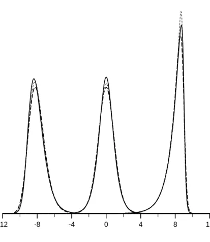
where φ and Φ are the standard normal density and distribution functions. Differences between (smooth) densities are, in any case, not very marked. See Fig. 1 for three sets of log F, hyperbolic and normal-based densities (the latter computed numerically), all normalised to have unit variance and means strategically placed along the line to allow clarity of viewing. What differences there are between densities show up mainly in the centres of the distributions.
* * * Fig. 1 about here * * *
My colleague Karim Anaya made the excellent observation thatH[2](x)≡
xH(x) +h(x) has the properties of a first iterated left-tail distribution func-tion, provided again that the otherwise arbitrary density function h (and distribution function H) are such thath is not ‘very heavy left-tailed’ in the sense described in Section 1. The distribution function associated with H[2]
is, of course, not H but H(x) +xh(x) +h(x), which differs from H except in the case H = Φ. However, this method of construction of G[2]’s tends to add complication and so no examples will be pursued.
3·6. Three-piece distributions
The asymmetric Laplace distribution is a two-piece distribution in the sense that its density can be thought of as being made up of two smooth parts joined together continuously but, in this case, not differentiably. If I drop the requirement thatGbe symmetric and employ instead a distribution onR+, further two-piece distributions ensue, but they will not be considered here.
Instead, consider G to be a symmetric distribution on finite support (which, without loss of generality, I shall take to be (−1,1)). These re-sult in three-piece distributions. The simplest case is that G be uniform so that G(x) = (1/2)(1 +x)I(−1 < x < 1) +I(x ≥ 1). It follows that
G[2](x) = (1/4)(1 +x)2I(−1< x < 1) +xI(x≥1) and thence that
fU(x)∝ exp(αx) if x <−1, exp−ααβ+βexp −(1/4)(α+β)x− αα−+ββ2 if −1≤x <1, exp(−βx) if x≥1. (6)
KU(α, β) = 1 αe −α+ 1 βe −β + 2 π α+β exp − αβ α+β Φ β 2 α+β −Φ −α 2 α+β .
Density (6) is the result of the very simple piecewise method of continuously — but not differentiably — joining two lines and a quadratic centre on the log density scale. Equivalently, it consists of a normal centre on to which exponential, rather than normal, tails have been grafted. In the symmetric case with α = β, (6) is the density associated with the ‘most robust’ M-estimator of Huber (1964, p.75; rescale (6) by factor k and take α = k2 to match Huber’s parameterisation).
Higher order contact between pieces can be achieved by replacing the quadratic by a higher order polynomial by, for example, replacing uniform
g by other symmetric beta g(x) ∝ (1−x2)m−1I(−1 < x < 1) for integer
m >1. See also Section 6.
4. Related distributions I: limiting cases
For the purposes of this section, consider
1 σfG x−µ σ = 1 σKG(α, β)exp α(x−µ) σ −(α+β)G [2]x−µ σ (7)
with (symmetric) G not being a degenerate distribution. It turns out that one can take µ= 0 in Sections 4.1 and 4.2.
4·1. α, β →0
Immediately, the asymmetric Laplace is the limiting form of (7) obtained by letting σ tend to zero. This normalisation is, clearly, appropriate for the situation where α, β →0. In particular, in the symmetric case ofα=β with limiting (symmetric) Laplace distribution, one can take σ =α.
4·2. α=β → ∞ From (7) with α=β, KG(α, α) = ∞ −∞exp{α(x−2G [2](x))}dx = exp(−2αG[2](0)) ∞ −∞exp[α{x−2(G [2](x)−G[2](0))}]dx exp(−2αG[2](0)) ∞ −∞exp{−αx 2g(0)}dx = exp(−2αG[2](0)) π αg(0),
the Taylor approximation being justified by the integrand in the second line being 1 for x = 0 and vanishingly small otherwise. (Note that 2G[2](0) =
E(|XG|) which has already implicitly been assumed to exist.) Now take
σ =2αg(0). Then, −logσ−logfG x σ −1 2log(2π) + α 2g(0)x −2α G[2] x 2αg(0) −G[2](0) −1 2log(2π)− 1 2x 2
and the standard normal distribution ensues.
4·3. α→ ∞, β fixed
Define (x)> 0 to be the limiting expression for G[2](x)−x as x → ∞. Take µandσ large such thatα ((x−µ)/σ)∼ 1(x)>0 for largexand some function 1. Then, the exponential part of (7) is
exp −β(x−µ) σ −(α+β) G[2] (x−µ) σ − (x−µ) σ
and this affords a limiting density of the form
on appropriate support.
Formula (8) works for the asymmetric Laplace distribution because then
1(x) = 0 and the limiting case as the left-hand tail parameter α→ ∞is, of
course, the exponential distribution on R+. (Ditto for all distributions gen-erated by g’s on finite support.) For the log F distribution, the appropriate normalisation is µ = −logα, σ = 1, so that 1(x) = e−x and the limiting density is proportional to e−βxexp(−e−x), x ∈ R. This Gumbel extreme
value limiting distribution corresponds to the log F’s interpretation as an order statistic distribution (Jones, 2004, Section 4.6). It is a consequence of the logistic’s exponential tails and the same limiting distribution applies to e.g. the doubly double exponential distribution. For the hyperbolic distri-bution, take µ= 0, σ = 4/α, so that the limiting density is proportional to exp{−(βx+ (1/x))}, x ∈ R+. This is the positive hyperbolic distribution (e.g. Barndorff-Nielsen and Blaesild, 1983, whose formula (7) incorporates a scale parameter).
5. Maximum likelihood estimation I: too many scale parameters
Let X1, ..., Xn be an i.i.d. sample from the location-scale version (7) of density fGand assume thatGis twice continuously differentiable. The asym-metric Laplace distribution is therefore disqualified from consideration on two counts, the second being the lack of a role for σ which cannot be sep-arated from α and β in that case. (See Section 3.5 of Kotz, Kozubowski and Podg´orski, 2001, for a full account of maximum likelihood estimation for the asymmetric Laplace distribution.) The (exact) unidentifiability of α,
β and σ in the asymmetric Laplace case suggests that there might be what might be called a practical unidentifiability of α, β and σ in other cases of
fG. This proves to be so in the sense that the asymptotic correlation between the maximum likelihood estimators of at least one pair of these parameters is necessarily extremely high and therefore that there is no hope of estimat-ing all these parameters well from data, nor indeed is there any need to: in practice, one parameter can be dropped. This is because α, β and σ all act as scale parameters, yet there are clear roles for only two scale parame-ters, one associated with the left-tail of the distribution, the other with the right (or perhaps one overall scale parameter and one parameter controlling
the left-right difference). Relatedly, the tails of σ−1fG(σ−1(x−µ)) go like
e(α/σ)x as x→ −∞and e−(β/σ)x as x→ ∞.
The elements of the observed and expected information matrices associ-ated with maximum likelihood estimation in the four-parameter distribution (7) are given in the Appendix. The main point concerning the unnecessary nature of one of the scale parameters can, however, be demonstrated clearly in the symmetric three-parameter case with α=β, as follows. The symme-try of the distribution means that the location estimate ˆµ is asymptotically independent of ˆσ and ˆα. Using manipulations similar to those underlying the Appendix, the elements of the submatrix of the expected information matrix associated with ˆσ and ˆα are n times
Jσσ = 1 σ2(1 + 2αE(X 2 FGg(XFG))), Jσα =− 1 σα and Jαα =M G(α)
where MG(α) = log(KG(α, α)). The asymptotic correlation, r say, of ˆσ and ˆ
α is therefore the following function of α only:
r(α) = 1
α{MG(α)(1 + 2αE(XF2Gg(XFG)))}1/2. (9)
When α → ∞, the manipulations at the start of Section 4.2 can be ex-tended to show thatMG(α)∼1/(2α2) andE(XF2Gg(XFG))∼1/(2α) so that limα→∞r(α) = 1. An asymptotic approximation of 1 for limα→0r(α) also seems to arise from other calculations. Indeed, an extraordinary closeness of r(α) to unity for all α is obtained in numerical calculations. For the log
F and hyperbolic distributions, the minimum correlations that I obtained numerically were 0.992 and 0.994, respectively! I did a similar analysis for the four-parameter log F distribution in Jones (2006a) and obtained a (now rather less impressive!) minimum correlation between ˆσ and each of ˆα, ˆβ and 2/( ˆα+ ˆβ) of “almost 0.9”.
Treating the log F distribution as a three parameter distribution must alleviate the computational problems noted with fitting the four-parameter distribution by Brown et al. (1996) and Dupuis (2001). For more on the the-ory of maximum likelihood estimation for the logF distribution see Prentice (1975) and for the hyperbolic distribution see Barndorff-Nielsen and Blaesild (1981).
6 Maximum likelihood estimation II: kernel quantile estimation
The first likelihood equation readsn−1ni=1G((Xi−µ)/σ) =α/(α+β) or equivalently n−1 n i=1 G µ−Xi σ = β α+β ≡p. (10)
The left-hand side of (10) is nothing other than the kernel estimator of the distribution function at the point µ with bandwidth σ and kernel distri-bution function G. Solving (10) for µ, the resulting ˆµ(p) is precisely the inversion kernel quantile estimator at p (Nadaraya, 1964, Azzalini, 1981). It is well known that maximum likelihood location estimation in the asym-metric Laplace distribution is equivalent to sample quantile estimation (e.g. Koenker and Machado, 1999); here, for the first time, is a simple general-isation to the case of kernel smoothed quantile estimation. It is somewhat intriguing to note that the more tractable choices of G from a distribution theory perspective and the usual preferred choices of G from a kernel es-timation perspective (e.g. normal and Epanechnikov and other symmetric beta kernels; Sections 3.5 and 3.6) differ. However, the relative indifference to precise choice of kernel, bar perhaps smoothness considerations, matches with the relative similarity of members of the class fG as in Fig. 1.
Define α+β = δ and fix p by choice of quantile. In this parametrisa-tion, the tails of the underlying density go like e(1−p)(δ/σ)x as x → −∞ and
e−p(δ/σ)x asx→ ∞.This makes it clear (again) that σ and δ are both acting
as scale parameters, but for current purposes it is appropriate to set δ = 1 (and hence completely fix α and β as 1−p and p, respectively) and retain
σ, formula (10) still holding. Interestingly, the special case of the log F dis-tribution with δ = 1 that corresponds to use of the logistic kernel in (10) is precisely the NEF-GHS (natural exponential family generalized hyperbolic secant) distribution of Morris (1982). In addition, when p = 1/2, Huber’s ‘most robust’ location M-estimator mentioned in Section 3.6 can now be newly interpreted as an inversion kernel median estimator using a uniform kernel.
But now we also have a (semi-)principled method of bandwidth selection by choosing σ and µ simultaneously by maximum likelihood (in the model with δ = 1). The second likelihood equation that should be solved in
con-junction with (10) is 1 n n i=1 (Xi−µ) p−G µ−X i σ =σ. (11)
Uniqueness of the estimators of µand σ is assured. In fact, it can be shown that the left-hand sides of (10) and (11) are monotone decreasing in µ for fixed σ and in σ for fixed µ, respectively, over appropriate ranges of values and hence that simple (e.g. bisection) methods can be used successfully to compute ˆµ and ˆσ.
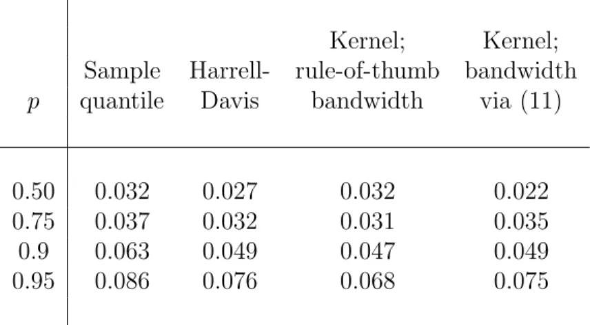
Simulation results using this methodology are, however, mixed. As an ex-ample, Table 1 gives results forn = 50 and the standard normal distribution; results forn= 100 and other distributions are qualitatively similar. The four methods compared in Table 1 are the sample quantile, the Harrell and Davis (1982) estimator and two estimators based on (10) with logistic G: the first takes σ to be the ‘rule-of-thumb’ bandwidth associated with minimisation of asymptotic mean squared error (Azzalini, 1981) assuming normality — which is in fact the right assumption here; the second utilises (11). Taking 50,000 replications resulted in standard errors such that the simulated mean squared errors are (approximately) correct to the number of decimal places shown.
* * * Table 1 about here * * *
The kernel method with σ chosen by (11) performs particularly well at the median. This is because we are fitting a smooth symmetric log F distri-bution rather than the sample quantile’s implicit Laplace distridistri-bution. This, of course, can also be considered to be good robust estimation of location via a particular M-estimator. Performance is rather worse for other quan-tiles. The new estimator proves to be of roughly comparable quality to the Harrell-Davis estimator (which is well thought of in the study of Sheather and Marron, 1990) but not as good as the rule-of-thumb kernel estimator (whose good performance persists for non-normal distributions). It struggles particularly when p = 0.75 but seems to improve again for higher p. The somewhat disappointing overall performance of the new estimator away from the median must be associated with the fitting of particular skew logF distri-butions that bear little relation to the symmetric distribution underlying the data (although the same is true of the asymmetric Laplace distribution un-derlying the sample quantile). Hence the words “a (semi-)principled method of bandwidth selection” above!
It is intended to explore the consequences of the above for kernel quantile regression elsewhere.
7. Related distributions II: exponential tails and power tails
In this section, I will briefly explore distributions related tofG by simple transformation.
7·1. Distributions with power tails on R+
Probably the most obvious transformation link to make is that associated with ‘taking logs’. LetY =eX,X = logY. Then the densityfG;+,p(y),y >0, of Y has the form
fG;+,p(y) = y
α−1
KG(α, β)
exp{−(α+β)G[2](log(y))}. (12) In this way, the simple exponential tails of density fG translate to simple power tails for fG;+,p(y):
fG;+,p(y)∼yα−1 as y→0, fG;+,p(y)∼y−(β+1) asy→ ∞.
Elsewhere (Jones, 2006b) I have argued that this behaviour at 0 — that of the reciprocal of a random variable with ay−(α+1) right-hand density tail —
is the natural analogue of the power tail at infinity. Formula (12) might be seen as directly generating densities with power tails on R+ starting from a simple symmetric distribution on R.
Immediately and unsurprisingly, the power-tailed distribution associated with the log F distribution on R is the F distribution on R+. The distri-bution associated with fH is known as the log hyperbolic distribution and it is in that guise that it is most often used as a model for (positive) data (e.g. Barndorff-Nielsen, 1977). The distribution associated with fAL has the simple two-piece density given by
fAL;+,p(y) = αβ
α+β
yα−1I(0< y < 1) +y−(β+1)I(y≥1);
Fieller, Flenley and Olbricht (1992) put this ‘log-skew-Laplace’ distribution forward as a more tractable alternative to the log hyperbolic distribution. Further distributions with power tails onR+ can, of course, be derived from other examples of fG.
7·2. Distributions with power tails on R
In Jones (2006b), I argued that the following simple transformation from
Y ∈ R+ toZ ∈ R has the useful property of maintaining the power tails of
fG;+,p(y) in the density fG;p(z), say:
Z = 1 2 Y − 1 Y = sinh(log(Y)). (13) Combining this transformation with the exponential transformation to Y
from X leads to densities with power tails on R in the sense that
fG;p(z)∼z−(α+1) asz → −∞, fG;p(z)∼z−(β+1) as z → ∞.
But the combined transformation is nothing other than Z = sinh(X). And the associated density is
fG;p(x) =KG−1(α, β)(z+ √ 1 +z2)α √ 1 +z2 exp{−(α+β)G [2](sinh−1(z))}. (14)
The density generated by logisticG is particularly interesting:
fLF;p(z) = 1
B(α, β)
(z+√1 +z2)α
√
1 +z2(1 +z+√1 +z2)α+β.
This is the k = 1 special case of distribution (6.2) of Jones (2004) and, as such, is, when α and β are integers, the distribution of an order statistic of a random sample from the distribution with density
z+√1 +z2
√
1 +z2(1 +z+√1 +z2)2.
(It is also interesting to note that the (scaled)t2distribution is nothing other than the distribution of sinh(L/2) where L follows the logistic distribution, a simple relationship buried in Jones, 2004, but missed by Jones, 2002.) The two-piece distributions associated with the asymmetric Laplace distribution have density
fAL;p(z) = αβ (α+β)√1 +z2
Taking logs and sinhs ofX’s with particular distributions, different from those considered here, is at the heart of the Johnson system of distributions (Johnson, 1949, Johnson, Kotz and Balakrishnan, 1994a, Section 12.4.3). See Jones (2006b) for material on the interplay between Johnson distributions and transformation (13).
7·3. Distributions with exponential tails on R+
The inverse of transformation (13),Y =X+√1 +X2 = exp(sinh−1(X)),
can also be applied to densities with exponential tails on R to ‘maintain’ exponential tails on R+ in the sense that
fG;+,e(y)∼y−2e−α/(2y) as y→0, fG;+,e(y)∼e−(β/2)y as y→ ∞.
(The extra scaling factor of 1/2 is inconsequential.) The ‘exponential tail behaviour’ at zero is actually that of the reciprocal of a random variable with exponential tail behaviour at infinity and is also rather similar to that of the inverse Gaussian distribution, for which the power −2 is replaced by
−3/2.
To cut a longer story short, probably the most attractive distribution in this family turns out to be that associated with the hyperbolic distribution:
fH;+,e(y) = 1 2KH(α, β) 1 + 1 y2 exp 1 2 −α y −βy .
This is a mixture of the positive hyperbolic distribution and its version weighted by 1/y2, with mixture probabilitiesα/(α+β) andβ/(α+β), respec-tively. However, this is in competition with the log hyperbolic distribution itself which arises from the limiting process of Section 7.3 and behaves as
e−1/y asy→0 (as well ase−βy asy → ∞.). Note, however, that the limiting
process approach is less general than the transformation approach in that not all limiting densities (8) have support R+. A class of cases that have the required support arises from g having power upper tail x−(γ+1), γ > 1, for
Acknowledgement
I am very grateful to Karim Anaya for his considerable interest and ex-cellent suggestions and to Frank Critchley for an interesting question.
Appendix
Observed and expected information for the four-parameter case
WriteMG(α, β) = logKG(α, β). Based on the log-likelihood
−nlogσ−nMG(α, β) +α n i=1 (Xi−µ) σ −(α+β) n i=1 G[2]Xi−µ σ ,
it can readily be shown that the elements of the observed information matrix (minus the second derivative of the log-likelihood) in the four-parameter case are as follows: ιµµ = (α+β) σ2 n i=1 g X i−µ σ ; ιµσ = (α+β) σ2 n i=1 (Xi−µ) σ g X i−µ σ ; ισσ= 1 σ2 n+ (α+β) n i=1 (Xi−µ)2 σ2 g X i−µ σ ; ιµα= 1 σ n−n i=1 G X i−µ σ = βn (α+β)σ; ιµβ =−1 σ n i=1 G X i−µ σ =− αn (α+β)σ; ισα = 1 σ n i=1 (Xi−µ) σ 1−G X i−µ σ = n (α+β)σ β( ¯X−µ) σ −1 ; ισβ =−1 σ n i=1 (Xi−µ) σ G X i−µ σ =− n (α+β)σ 1 +α( ¯X−µ) σ ; ιαα=nM20G(α, β); ιαβ =nM11G(α, β) ιββ =nM02G(α, β). Here, ¯X=n−1ni=1Xi as usual.
It is clear that, on taking expectations, the elements of the expected infor-mation matrix are of the forms n times jµµ/σ2, jµσ/σ2, jσσ/σ2, jµα/σ, jµβ/σ,
jσα/σ,jσβ/σ,jαα,jαβ and jββ, respectively, where thej’s are functions of α and
β only. Thej’s look much like theι’s above except that the first three depend on
E(XFrGg(XFG)), r= 0,1,2, and E(( ¯X−µ)/σ) =M10G(α, β)− M01G(α, β). There-fore, the expected information matrix does not depend onµat all and asymptotic
correlations are independent ofσ too.
References
Azzalini, A. (1981). A note on the estimation of a distribution function and quantiles by a kernel method. Biometrika 68, 326–8.
Barndorff-Nielsen, O. (1977). Exponentially decreasing distributions for the logarithm of particle size. Proc. Roy. Soc. London, Ser. A353, 401–19. Barndorff-Nielsen, O. & Blaesild, P. (1981). Hyperbolic distributions and ramifications: contributions to theory and application. In Statistical Distributions in Scientific Work, Vol. 4, Eds. C. Taillie et al., pp. 19– 44. Reidel.
Barndorff-Nielsen, O. & Blaesild, P. (1983). Hyperbolic distributions. In
Encyclopedia of Statistical Sciences, Eds. N.L. Johnson, S. Kotz and C.B. Read, pp. 700–7. New York: Wiley.
Bassan, B., Denuit, M. & Scarsini, M. (1999). Variability orders and mean differences. Statist. Probab. Lett. 45, 121–30.
Brown, B.W., Spears, F.M., Levy, L.B., Lovato, J. & Russell, K. (1996). Algorithm 762: LLDRLF, likelihood and some derivatives for
log-F models. ACM Trans. Math. Software 22, 372–82.
Dupuis, D.J. (2001). Fitting log-F models robustly, with an application to the analysis of extreme values. Comput. Statist. Data Anal. 35, 321– 33.
Fieller, N.R.J., Flenley, E.C. & Olbricht, W. (1992). Statistics of particle size data. Appl. Statist. 41, 127–46.
Gumbel, E.J. (1958). Statistics of Extremes. New York: Columbia Univer-sity Press.
Harrell, F.E. & Davis, C.E. (1982). A new distribution-free quantile estima-tor. Biometrika69, 635–40.
Huber, P.J. (1964). Robust estimation of a location parameter. Ann. Math. Statist. 35, 73–101.
Johnson, N.L. (1949). Systems of frequency curves generated by methods of translation. Biometrika 36, 149–76.
Johnson, N.L., Kotz, S. & Balakrishnan, N. (1994). Continuous Univariate Distributions, Vol. 1, Second Edition. New York: Wiley.
Jones, M.C. (2002). Student’s simplest distribution. Statistician51, 41–9. Jones, M.C. (2004). Families of distributions arising from distributions of
order statistics (with discussion). Test 13, 1–43.
Jones, M.C. (2006a). The logistic and the log F distribution. In Hand-book of the Logistic Distribution, Second Edition, Ed. N. Balakrish-nan, New York: Dekker, to appear. Open University Department of Statistics Technical Report 06/01; see http://statistics.open.ac.uk/ TechnicalReports/TechnicalReportsIntro.htm
Jones, M.C. (2006b). Connecting distributions with power tails on the real line, the half line and the interval. Under consideration. Open Uni-versity Department of Statistics Technical Report 05/12; see http:// statistics.open.ac.uk/TechnicalReports/TechnicalReportsIntro.htm Jones, M.C. & Faddy, M.J. (2003). A skew extension of the t distribution,
with applications. J. Roy. Statist. Soc. Ser. B 65, 159–74.
Koenker, R. & Machado, J.A.F. (1999). Goodness of fit and related inference processes for quantile regression. J. Amer. Statist. Assoc. 94, 1296– 310.
Kotz, S., Kozubowski, T.J. & Podg´orski, K. (2001). The Laplace Distribu-tion and GeneralizaDistribu-tions; A Revisit With ApplicaDistribu-tions to Communica-tions, Economics, Engineering, and Finance. Boston: Birkhauser. Morris, C.N. (1982). Natural exponential families with quadratic variance
functions. Ann. Statist. 10, 65–80.
Nadaraya, E.A. (1964). Some new estimates for distribution functions. Theor. Probab. Applic. 15, 497–500.
Prentice, R.L. (1975). Discrimination among some parametric models.
Biometrika62, 607–14.
Sheather, S.J. & Marron, J.S. (1990). Kernel quantile estimators. J. Amer. Statist. Assoc. 85, 410–16.
Table 1: Mean squared errors associated with the estimation of normal quan-tiles from samples of size n = 50for specified pand four estimation methods. The logistic kernel was used in the kernel methods. 50,000 replications
Kernel; Kernel; Sample Harrell- rule-of-thumb bandwidth
p quantile Davis bandwidth via (11)
0.50 0.032 0.027 0.032 0.022 0.75 0.037 0.032 0.031 0.035 0.9 0.063 0.049 0.047 0.049 0.95 0.086 0.076 0.068 0.075
Fig. 1: Log F (solid), hyperbolic (dashed) and normal-based (dotted) distri-butions with variance unity and β = 2 with, from left, means −8,0 and 8 and α = 8, 2 and 0.25, respectively.