Inference of high-dimensional linear models with time-varying coefficients

(1)

c

(2)

INFERENCE OF HIGH-DIMENSIONAL LINEAR MODELS WITH TIME-VARYING

COEFFICIENTS

BY

YIFENG HE

DISSERTATION

Submitted in partial fulfillment of the requirements

for the degree of Doctor of Philosophy in Statistics

in the Graduate College of the

University of Illinois at Urbana-Champaign, 2018

Urbana, Illinois

Doctoral Committee:

Professor Xiaohui Chen, Chair

Professor Yuguo Chen

Professor Annie Qu

(3)

Abstract

In part 1, we propose a pointwise inference algorithm for high-dimensional linear models with time-varying coefficients and dependent error processes. The method is based on a novel combination of the nonparamet-ric kernel smoothing technique and a Lasso bias-corrected ridge regression estimator using a bias-variance decomposition to address non-stationarity in the model. A hypothesis testing setup with familywise error control is presented alongside synthetic data and a real application to fMRI data for Parkinson’s disease.

In part 2, we propose an algorithm for covariance and precision matrix estimation high-dimensional transpose-able data. The method is based on a Kronecker product approximation of the graphical lasso and the application of the alternating directions method of multipliers minimization. A simulation example is provided.

(4)

Introduction

Between 2005 and 2015, humanity watched its aggregate data multiply 10-fold every 2 years, a pattern driven by automated data collection and advances in technology such as the falling cost of digital storage. It has become cheaper and easier to gather everything than to consider what specific data to target and collect. We cast increasingly larger nets in search of the golden fish to explain some phenomena of interest. Online retailers log thousands of details about their customers to provide more personalized services. Genomics and fMRI machines produce massive parallel datasets in an effort to better understand patients and disease. Financial institutions collect vast arrays of data to produce better alpha for their investors. Over time, we have seen the fields of technology, medicine, finance, and others embrace the collection and analysis of large scale data.

Such an explosion has resulted in friction with traditional statistical theory, where it is typically assumed that one is working with a large number of samples but only a handful of well chosen, relevant variables. Since modern data collection relinquishes domain expertise in favor of a systematic approach by storing all available information about customers, patients, and subjects, we are left with a large number of variables rather than the handful from classical statistics. These numbers skyrocket even higher when we introduce functions of existing variables such as interaction effects orn-tuples. Therefore, there is great interest in the statistical analysis of problems where the number of variables or dimensions (p) in data exceeds its sample size (n), a domain referred to ashigh-dimensional statistics.

1.1 The Curse of Dimensionality

The primary obstacle in high-dimensional statistics is the curse of dimensionality, a term coined by Richard Bellman to describe the rapid growth of an optimization problem’s complexity with dimensionality, originally in the context of exhaustive enumeration in a product space. [Bellman, 1961]

(6)

Rp and the corresponding responsesY1, ..., Yn∈Rgiven by

Yi=f(Xi) +ei

where f is L-Lipschitz and ei ∼ i.i.d. N(0,1). Let F be the functional class of all Lipschitz func-tions on [0,1]p _{and ˆ}_f _{be some estimator of} _f _{using the observed responses.} _{Minimax decision theory} [Ibragimov and Khasminskii, 1981] shows that for any estimator ˆf, we have

sup f∈FE ˆ f(X)−f(X) 2 ≥Cn−2/(2+p) , n→ ∞

whereC is a constant which depends on the Lipschitz constantL. This very slow rate of convergence in high-dimensions is the price of the curse of dimensionality. In order to estimatef to an accuracy ofin the example above, we would needO −(2+p)/2

samples. Therefore, the appetite for data grows exponentially with the number of variablesp.

1.2 The Blessing of Dimensionality

The blessing of dimensionality is driven by the concentration of measure phenomenon. Generally speaking, the concentration of measures states that Lipschitz functions such as the average of bounded, independent random variables are concentrated around their expectations.

Take, for example, the concentration of Lipschitz functions of Gaussian random variables [Donoho, 2000]. Let (X1, ..., Xn) be a vector of i.i.d. Gaussian random variables andf :Rp→RisL-Lipschitz with respect

to thel2 metric. Then the random variablef(X)−E[f(X)] is sub-Gaussian such that

Ph|f(X)−E[f(X)]| ≥ i ≤2 exp − 2 2L2

Therefore, a Lipschitz function of standard Gaussian random variables is nearly constant and the tails, at worst, behave like a scalar Gaussian variable with varianceL2_{, regardless of dimension.}

Similar tools exist for the concentrations of product measures with respect tol1 and Hamming metrics,

uniform measures over the unit sphere surface with respect to l2, and others. These concentrations of

measures are heavily used to establish theoretical results in high-dimensional statistics, most commonly for the bounding of error probabilities.

(7)

1.3 High-Dimensional Linear Regression

In the traditional linear regression model, we are given predictor measurements X1, ..., Xn ∈ Rp and the

responsesY1, ...Yn ∈Rto be modeled by

Y =Xβ+e

where X= (X₁>, ..., X_n>)> ∈ Rn×p is the design matrix, Y ∈ Rn the response vector, e∈Rn the noise or

error vector, andβ ∈Rp the coefficient vector to be estimated. Typically,e is assumed to be independent

ofXwith mean zero.

To claim that the ordinary least squares (OLS) estimator has been well studied in low-dimensions would be an understatement, but in the case wheren > p, the OLS estimator can be written as

ˆ

βOLS= (X>X)−1X>Y

This is well defined where the columns of X are linearly independent but this assumption clearly cannot hold when p > n such that X>X is singular. Therefore the parameter estimation problem is ill-posed in high-dimensions.

Furthermore in the simple case whereei are i.i.d. with varianceσ2, the OLS linear regression estimator has expected prediction error σ2+pσ2/n with zero bias. Therefore, adding an additional variable Xp+1

contributes an extraσ2/nto the variance, regardless if said variable is linearly relevant (i.e. βp+1= 0). We

can improve on the mean squared error (MSE) of our estimator by reducing the variance at the expense of introducing bias, such as though shrinkage where coefficients are coerced towards zero. This is of particular note in high-dimensions; While models may involve a large number of parameters such that p > n, there often exists an underlying low-dimensional structure such as sparsity or smoothness which makes inference a more realistic goal.

1.3.1 Ridge Regression

Regularization is a common tool used to address the issues of regression in high-dimensions which balances a loss function such as squared error in the context of linear regression with regularization or penalization to promote some underlying structure. Ridge regression [Hoerl and Kennard, 1970] is one of the simplest forms of regularization for linear models, and its coefficients ˆβRidge ∈Rp are defined by standardizing the

(8)

columns ofXand optimizing the following objective function

ˆ

βRidge= arg min β∈Rp

1

2kY −Xβk

2₊

λkβk2 (1.1)

where λ≥0 is a tuning parameter which controls the strength of shrinkage and the bias-variance tradeoff. The case of λ= 0 corresponds to the ordinary linear regression estimator where we have no bias but large variance. The case ofλ=∞shrinks all coefficients to ˆβRidge= 0, which has high bias but zero variance. In the simple case whereXis orthonormal, the shrinkage as a function ofλis given by

ˆ βRidge=

ˆ βOLS

1 +λ (1.2)

Furthermore, the existence property of the Ridge estimator guarantees the existence of someλ >0 such that the MSE of ˆβRidge is less than the MSE of ˆβOLS. However, finding or choosing such an appropriateλ is a somewhat contested topic, with cross-validation currently the most standard compromise.

A convenient property of the Ridge estimator is the differentiability of its objective function. As such, it’s easy to obtain a closed form solution within the rowspaceR(X).

ˆ

βRidge= (X>X) +λIp)−1X>Y (1.3) Bias( ˆβRidge) =−λ(X>X+λIp)−1β (1.4) Var( ˆβRidge) =σ2(X>X+λIp)−1X>X(X>X+λIp)−1 (1.5)

Therefore, the Ridge estimator ˆβRidgeis asymptotically biased and not a consistent estimator ofβ. While its distribution can be somewhat characterized, its bias still poses a challenge to performing statistical inference.

1.3.2 Lasso and Variable Selection

The Lasso [Tibshirani, 1996] also solves a similar penalized least squares regression problem using an l1

penalty, commonly with some assumption of sparsity.

ˆ

βLasso= arg min β∈R[

1

2kY −Xβk

2₊

λkβk1 (1.6)

Unlike the Ridge regression, the Lasso’s objective function is not differentiable and its solution does not necessarily have a closed form expression. However, there are many fast algorithms for obtaining the Lasso

(9)

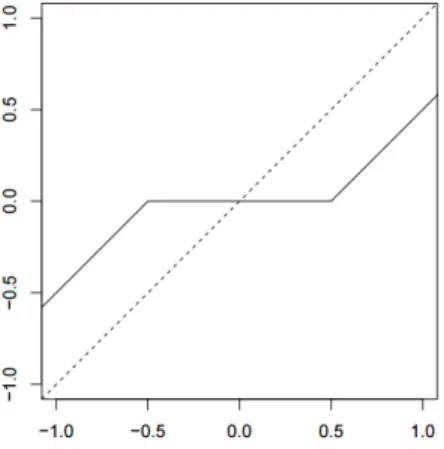
coefficients, and the effect of the regularization is essentially a soft-thresholding function.

Figure 1.1: A soft-thresholding function

Due to the nonlinear nature of the Lasso, its solution does not exist in the rowspace of X and its distribution is difficult to characterize. Since the soft-thresholding effect coerces some coefficients to zero, the Lasso effectively performs variable selection.

LetS0={j:βj6= 0, j= 1, ..., p} denote the active set and ˆS0 the estimated active set using a variable

selection technique such as the Lasso. The said method demonstrates model selection consistency if

P( ˆS0=S0)→1 p > n→ ∞ (1.7)

In the case of Lasso, model selection consistency requires a very strong set of assumptions on the design matrix referred to as the irrepresentable condition and the beta-min condition. Roughly speaking, the irrepresentable condition requires the columns of the design matrixXcorresponding to the active setS0 to

be nearly orthogonal to columns ofXcorresponding to the inactive setS₀C. As the name implies, the beta-min condition imposes a nonzero lower bound to|βj|, j∈S0. We refer to [Meinshausen and B¨uhlman, 2006]

and [Zhao and Yu, 2006] for a more detailed study of these assumptions. The irrepresentable condition can be relaxed to a restricted eigenvalue condition to obtain model screening consistency such that

P( ˆS0⊇S0)→1 p > n→ ∞ (1.8)

although the undesirable beta-min condition remains.

Furthermore, the Lasso yields an `2 consistent estimator [Meinshausen and Yu, 2009] under milder

as-sumptions with suitableλp

(10)

sparsity patterns cannot be recovered.

1.4 Statistical Inference in High-Dimensions

High-dimensional statistical theory has historically focused heavily on the estimation consistency, prediction consistency, oracle inequalities, and variable selection. The assessment of uncertainty such as assigning p-values in high-dimensional settings has remained an relatively poorly understood topic until only recently. The primary measure of uncertainty discussed here will be the p-value in the context of hypothesis testing for linear models. That is, for eachj∈1, ..., p, we are interested in testing

H0,j : βj = 0 Ha,j : βj 6= 0

We present several methods of assigning significance in high-dimensional linear models from current literature.

1.4.1 Multi-Sample Splitting

Multi-sample splitting or selective inference [Meinshausen et al., 2009] is a general two-step method of per-forming inference in high dimensions using a dimension reduction step and an inference in low-dimensions step.

Given a high-dimensional dataset with nobservations, multi sample splitting first partitions the indices {1, ..., n}into two parts denotedI1andI2with|I1|=bn/2c,|I2|=dn/2e, I1∪I2={1, ..., n}, andI1∩I2=∅.

LetYI_i and XI_i) denote, respectively, the elements of Y and the rows of Xcorresponding to the Ii index, i= 1,2. A variable screening procedure is applied on (YI₁,XI₁) to obtain ˆS0,I1 with cardinality|Sˆ0,I1| ≤ |I2|.

The Lasso is a common candidate for variable screening and implicitly satisfies the cardinality condition under weak assumptions. Indeed the choice of using roughly evenly sized partitions |I1| ≤ |I2| appears to cater

especially to the Lasso. While capable of screening consistency under stronger assumptions, a screening property is not always necessary for the construction of valid p-values [B¨uhlmann and Mandozzi, 2014].

Let X_I

2,Sˆ0,I1

denote the columns ofXI2 corresponding to the variables screened by ˆS0,I1. The second

step of the procedure simply regresses YI₂ ontoX_I

2,Sˆ0,I1

, which is readily solved by ordinary least squares regression and produces the desired p-values.

(11)

One glaring issue concerning the two-step selection and inference procedure is that the constructed p-values are very sensitive to the choice ofI1, I2, affectionately referred to by its authors as the p-value lottery.

The problem is somewhat addressed through repeated randomization in the sampling the partitions and aggregating the constructed p-values. Overall, the multi sample splitting approach is a generalized method with certain assumptions on variable screening and selection cardinality. However, the need for beta-min or zonal conditions for most screening methods runs counter to the purpose of a significance test. Additionally, its repeated sampling of partitions does not lend itself well to cases where complex dependencies exist in noise, such as spatio-temporal data.

1.4.2 Lasso Projection

The de-sparsified Lasso or low-dimension projection estimator (LPDE), proposed by [Zhang and Zhang, 2014] and [Dezeure et al., 2015] corrects the bias from Lasso using a projection onto a low-dimensional orthogonal space constructed using nodewise regression.

LetXj ∈Rn denote the column ofX corresponding to variablej= 1, ..., pandX−j ∈Rn×(p−1) denote

the other columns. LetZj∈Rn denote the residuals of the Lasso regression ofXj ontoX−j. Then, for any

Zj, Y>Zj X> jzj =βj+ X k6=j X>_kZj XjZjβk+ e>Zj X> j Zj (1.9) Therefore, the bias corrected plugin estimator using an initial Lasso estimate of β is

ˆ βj,LP DE= Y >_Z j X> jzj −X k6=j X> kZj XjZj ˆ βk,Lasso (1.10)

The LPDE estimator admits a Gaussian distribution under compatibility conditions on X, when the sparsity iss0=o(

√

n/log(p)), the rows ofXare i.i.d. N(0,Σ) with a positive lower bound on the eigenvalues of Σ, and Σ−1 is row-sparse. Aside from some somewhat undesirable assumptions on the fixed design, the LPDE estimator is very computationally demanding, roughly 2 orders of magnitude over multi-sample splitting and Ridge projection. On the other hand, it does not make any assumptions on the underlying β coefficients besides sparsity and achieves the Cramer-Rao efficiency bound, which the Ridge projection does not.

(12)

Chapter 2

Time-Varying High-Dimensional

Linear Models

2.1 Introduction

We consider the following time-varying coefficient models (TVCM)

y(t) =x(t)>β(t) +e(t) (2.1)

where t ∈[0,1] is the time index, y(·) the response process, x(·) the p×1 deterministic predictor process (i.e. fixed design), β(·) the p×1 time varying coefficient vector, and e(·) the mean zero stationary error process. The response and predictors are observed at evenly spaced time points ti = i/n, i = 1, ..., n, i.e. yi =y(ti),xi =x(ti) and ei =e(ti) with known covariance matrix Σe = Cov(e) where e= (e1,· · ·, en)>. TVCM is useful for capturing the dynamic associations in the regression models and longitudinal data analysis [Hoover et al., 1998] and it has broad applications in biomedical engineering, environmental science and econometrics. In this work, we shall consider the fixed design case and focus on thepointwiseinference for the time-varying coefficient vectorβ(t) in the high-dimensional double asymptotics framework min(p, n)→ ∞. Moreover, different from longitudinal setting, we consider only observations from one subject (xi, yi).

Nonparametric estimation and inference of the TVCM in the fixed dimension has been extensively stud-ied in literature, e.g. see [Robinson, 1989, Hoover et al., 1998, Fan and Wenyang, 1999, Zhang et al., 2002, Orbe et al., 2005, Zhang and Wu, 2012, Zhou and Wu, 2010]. In the high-dimensional setting, variable selec-tion and estimaselec-tion of varying-coefficient models using basis expansions have been studied in [Wei and Huang, 2010] and [Wang et al., 2014]. Nevertheless, our primary objective is not to estimateβ(t), but rather to perform the statistical inference on the coefficients. In particular, for any t ∈(0,1), we wish to test the following local hypothesis

H0,j,t:βj(t) = 0 VS H1,j,t:βj(t)6= 0, ∀j = 1,· · ·, p. (2.2) By assigning p-value at each time point, our goal is to construct a sequence of coefficient vectors that allows

(13)

us to assess the uncertainty of the dynamic patterns such as modeling the brain connectivity networks. Confi-dence intervals and hypothesis testing problems of lower-dimensional functionals of the high-dimensional con-stant coefficient vectorβ(t)≡β,∀t∈[0,1], have been studied in [B¨uhlmann, 2013], [Zhang and Zhang, 2014], and [Javanmard and Montanari, 2014]. To our best knowledge, little has been done for inference of dimensional TVCM. Therefore, our goal is to fill the inference gap between the classical TVCM and high-dimensional linear model.

As another key difference of this thesis from the existing inference literature on high-dimensional lin-ear models based on the fundamental i.i.d. error assumption [B¨uhlmann, 2013], [Zhang and Zhang, 2014], [Javanmard and Montanari, 2014], the second main contribution is to provide an asymptotic theory for an-swering the following question: To what extent can the statistical validity of a proposed inference procedure for i.i.d. errors hold for dependent error processes? Allowing temporal dependence is of practical interest since many datasets such as fMRI data are spatio-temporal in nature and the errors are correlated in the time domain. On the other hand, theoretical analyses reveal that the temporal dependence has delicate impact on the asymptotic rates for estimating the covariance structures [Chen et al., 2013]. Therefore, it is more plausible to build an inference procedure that is also robust in the time series context. The error processei is modelled as a stationary linear process

ei = ∞

X

m=0

amξi−m, (2.3)

where a0= 1 and ξi are i.i.d. mean-zero random variables (a.k.a. innovations) with variance σ2. Whenξi have normal distributions, linear processes of form (2.3) is a Gaussian processes that covers the auto-regressive and moving-average (ARMA) models with i.i.d. Gaussian innovations as special cases. For the linear process, we shall deal with both weak and strong temporal dependencies. In particular, if am=O(m−%), % >1/2, then ei is well-defined and it has: (i) short-range dependence (SRD) if % > 1; (ii) long-range dependence (LRD) or long-memory if 1/2< % <1. For the SRD processes, it is clear thatP∞

m=0|am|<∞and therefore

the long-run variance is finite.

The chapter is organized as follows. In Section 2.2, we describe our method in details. Asymptotic theory is presented in Section 2.3. In Section 2.4, we mention some practical implementation issues and extension of the noise model to more general non-Gaussian and heavy-tailed distributions. Section 2.5 presents some simulation results and Section 2.6 demonstrates a real application to an fMRI dataset. Proofs are available in the Appendix.

(14)

2.2 Method

2.2.1 Notations and Preliminary Intuition

Let K be a non-negative symmetric function with bounded support in [−1,1],R1

−1K(x)dx = 1 and bn be

a bandwidth parameter satisfies the natural condition bn = o(1) and n−1 = o(bn). For each time point t∈$= [bn,1−bn], the Nadaraya-Watson smoothing weight is defined as

w(i, t) =        K_bn(ti−t) Pn m=1Kbn(tm−t) if|ti−t| ≤bn 0 otherwise , (2.4)

whereKb(·) =K(·/b). Let Nt={i:|ti−t| ≤bn}be the bn-neighborhood of timet, |Nt|be the cardinality of the discrete setNt,Wt= diag(w(i, t)i∈N_t) be the|Nt| × |Nt|diagonal matrix with w(i, t), i∈Nton the diagonal, and Rt = span(xi :i ∈Nt) be the subspace inRp spanned by xi, the rows of design matrixX

in theNtneighborhood. Let Xt= (w(t, i)1/2xi)>_i∈N

t,Yt= (w(i, t)

1/2_yi)>

i∈Nt(i)and Et= (w(i, t) 1/2_ei)>

i∈Nt(i).

Then, the singular value decomposition (SVD) ofXtis

Xt=P DQ> (2.5)

where P and Q are |Nt| ×r, and p×r matrices such thatP>P =Q>Q=Ir. D = diag(d1,· · ·, dr) is a diagonal matrix containing thernonzero singular values of Xt. Now letPRt be the projection matrix onto Rt. Then, PRt=Xt>(XtX > t ) −_Xt₌_QQ> _(2.6) where (XtX> t )− =P D−

2_P>_{is the pseudo-inverse matrix of}_XtX>

t . Letθ(t) =PRtβ(t) be the projection of

β(t) ontoRt, the row subspace ofXtsuch thatB(t) =θ(t)−β(t) is the projection bias. Let

Ω(λ) = (Xt>Xt+λIp)−1Xt>W

1/2

t Σe,tW

1/2

t Xt(Xt>Xt+λIp)−1, (2.7) where Σe,t = Cov((ei)i∈Nt(i)), and Ωmin(λ) = minj≤pΩjj(λ) be the smallest diagonal entry of Ω(λ). For a generic vector b ∈_Rp_{, we denote} _|b|

q = (P p

j=1|bj|q)1/q if q > 0, and |b|0 = P

p

j=11(bj 6= 0) if q = 0. Denote w_t = infi∈Ntw(i, t) and wt = supi∈Ntw(i, t). For an n×n square symmetric matrix M and an n×mrectangle matrixR, we use ρi(M) andσi(R) to denote thei-th largest eigenvalues ofM and singular values of R, respectively. If k = rank(R), then σ1(R) ≥ σ2(R) ≥ · · · ≥ σk(R) > 0 = σk+1(R) = · · · =

(15)

σmax(m,n)(R), i.e. zeros are padded to the last max(m, n)−ksingular values. We denoteρmax(M),ρmin(M)

and ρmin6=0(M) be the maximum, minimum and nonzero minimum eigenvalues of M, respectively, and

|M|∞= max1≤j,k≤p|Mjk|. Let ρmax(M, s) = max |b|0≤s,b6=0 |b>_M_b| 2 |b|2 2 .

IfM is non-negative definite, thenρmax(M, s) is the restricted maximum eigenvalues ofM at mostscolumns

and rows.

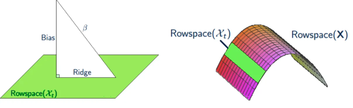
Before proceeding, we pause to explain the intuition behind our method. The p-dimensional coefficient vectorβ(t) is decomposed into two parts via projecting onto the|Nt|-dimensional linear subspace spanned by the rows ofXtand its orthogonal complement; see Figure 2.1(a). A key advantage of this decomposition is that the projected part can be conveniently estimated in the closed-form for example by ridge estimator since it lies in the row space ofXt and thus amenable for the subsequent inferential analysis. In the high-dimensional situation, this projection introduces a non-negligible shrinkage bias in estimating β(t) and therefore we may lose information becausep |Nt|. On the other hand, the shrinkage bias can be corrected by a consistent estimator ofβ(t). As a particular example, we shall use the Lasso estimator. However, any sparsity-promoting estimator attaining the same convergence rate as the Lasso should work. Because of the time-varying nature of the nonzero functionalβ(t), the smoothness on the row space of Xt along the time indextis necessary to apply nonparametric smoothing technique; see Fig. 2.1(b). As a special case when the nonzero componentsβ(t)≡βare constant functions and the error process is i.i.d. Gaussian, our algorithm is the same as [B¨uhlmann, 2013]. However, the emphases of this work are: (i) time-varying (i.e. non-constant) coefficient vectors; (ii) the errors are allowed to have heavy-tails by assuming milder polynomial moment conditions and to have temporal dependence, including both SRD and LRD processes. As mentioned earlier, there are other inferential methods for high-dimensional linear models such as [Zhang and Zhang, 2014] and [Javanmard and Montanari, 2014]. We do not explore specific choices here since the contribution is a general framework of combining nonparametric smoothing and bias-correction methods to make inference for high-dimensional TVCM. However, we expect that the non-stationary generalization would be feasible for those methods as well.

(16)

(a) Bias correction by projection to the row space ofXt.

(b) Smoothly time-varying row space ofXt.

Figure 2.1: Intuition of the proposed algorithm in Section 2.2.2.

2.2.2 Inference Algorithm

First, we estimate the projection biasB(t) by ˜B(t) = (PRt −Ip) ˜β(t), where ˜β(t) is the time-varying Lasso (tv-Lasso) estimator ˜ β(t) = arg min b∈Rp X i∈Nt w(i, t)(yi−x>_i b)2+λ1|b|1 (2.8) = arg min b∈Rp |Yt− Xtb|2 2+λ1|b|1.

Next, we estimateθ(t) =PRtβ(t) using the time-varying ridge (tv-ridge) estimator

˜ θ(t) = arg min b∈Rp X i∈Nt w(i, t)(yi−x>i b) 2₊_λ 2|b|22 = (X_t>Xt+λ2Ip)−1Xt>Yt. (2.9)

We shall defer the discussion of tuning parameters choice λ1 and λ2 in Section 2.3 and 2.4. Then, our

tv-Lasso bias-corrected tv-ridge regression estimator forβ(t) is constructed as

ˆ

β(t) = ˜θ(t)−B(t).˜ (2.10)

Now, based on ˆβ(t) = ( ˆβ1(t),· · ·,βˆp(t))>, we calculate the raw two-sided p-values for individual coefficients

˜ Pj = 2 " 1−Φ | ˆ βj(t)| −λ1₁−ξmaxk6=j|(PRt)jk| Ω1_jj/2(λ2) !# , j = 1,· · · , p, (2.11)

(17)

whereξ∈[0,1) is user pre-specified number, which depends on the number of nonzeroβ(t), i.e. sparsity. In particular, if|supp(β(t))|is bounded, then we can chooseξ= 0. Generally, following [B¨uhlmann, 2013], we useξ= 0.05 in our numeric examples to allow the number of nonzero components inβ(t) diverges at proper rates. Letv(t) = (V1(t),· · · , Vp(t))>∼N(0,Ω(λ2)) and define the distribution function

F(z) =P min j≤p2 h 1−ΦΩ−_jj1/2(λ2)|Vj(t)| i ≤z . (2.12)

We adjust the ˜Pjfor multiplicity byPj =F( ˜Pj+ζ), whereζis another predefined small number [B¨uhlmann, 2013] that accommodates asymptotic approximation errors. Finally, our decision rule is defined as: RejectH0,j,t ifPj ≤αforα∈(0,1). For i.i.d. errors, since Σe=σ2Idn and

Ω(λ2) =σ2(Xt>Xt+λ2Ip)−1Xt>WtXt(Xt>Xt+λ2Ip)−1,

we see that F(·) is independent of σ. Therefore, F(·) can be easily estimated by repeatedly sampling from the multivariate Gaussian distribution N(0,Ω(λ2)). Similar observations have been pointed out in

[B¨uhlmann, 2013].

2.3 Asymptotic Results

In this section, we present the asymptotic theory of the inference algorithm in Section 2.2.2. First, we state the main assumptions for i.i.d. Gaussian errors.

1. Error. The errorsei∼N(0, σ2) are independent and identically distributed (i.i.d.).

2. Sparsity. β(·) is uniformlys-sparse, i.e. sup_t∈[0,1]|S0t| ≤s, whereS0t={j:βj(t)6= 0}is the support set.

3. Smoothness.

(a) β(·) is twice differentiable with bounded and continuous first and second derivatives in the coordinate-wise sense, i.e. βj(·)∈ C2_([0,_{1], C}

0) for eachj = 1,· · ·, p and C0 is an upper bound

for the partial derivatives.

(b) Thebn-neighborhood covariance matrix ˆΣ_t =|Nt|−1P

i∈Ntxix>i :=Xt >_X

t satisfies the following conditions:

ρmax( ˆΣt, s)≤ε −2

(18)

4. Non-degeneracy.

lim inf

λ↓0 Ωmin(λ)>0. (2.14)

5. Identifiability.

(a) The minimum nonzero eigenvalue condition

ρmin6=0( ˆΣt)≥ε

2

0>0. (2.15)

(b) Therestricted eigenvalue conditionis met:

φ0= inf ( φ >0 : min |S|=s inf |bSc|1≤3|bS|1 b>Σˆtb |bS|2 1 ≥φ 2

s holds for allt∈[0,1]

)

>0, (2.16)

where ˆΣt=X>

t Xtis the kernel smoothed covariance matrix of the predictors.

6. Kernel. The kernel function K(·) is non-negative, symmetric around 0 with bounded support in [−1,1].

Here, we comment the assumptions and their implications. Assumption 1 and 6 are standard. The Gaussian distribution is non-essential and it can be relaxed to sub-Gaussian and heavier tailed distributions; see Section 2.4 for more discussions. Assumption 2 is a sparsity condition for the nonzero functional components and we allows→ ∞slower than min(p, n). It is a key condition for maintaining the low-dimensional structure when the dimensionpgrows fast with the sample sizen. In addition, by the argument of proving [Zhou et al., 2010, Theorem 5], it also implies that the number of nonzero first and second derivatives of β(t) is bounded by s almost surely on [0,1]. Assumption 3 ensures the smoothness of the time-varying coefficient vector and the design matrix so that nonparametric smoothing techniques are applicable. Examples of assumption 3(a) include the quadratic formβ(t) =β+αt+ξt2_{/2 and the periodic functions}_β_{(t) =}_β₊_α_sin(t)+_ξ_{cos(t) with}

|α|∞+|ξ|∞≤C0. Assumption 3(b) can be viewed as the Lipschitz continuity on the local design matrix that

is smoothly evolving [Zhou and Wu, 2010]. However, it is weaker than the condition thatρmax( ˆΣt)≤ε −2 0

because the latter may grow to infinity much faster than the restricted form (2.13).

Assumption 4 is required for non-degenerated stochastic component of the proposed estimator which is used for the inference purpose. Assumption 5(a) and 5(b), i.e. (2.15) and (2.16), together impose the identifiability conditions for recovering the coefficient vectors. Analogous condition of the time-invariant

(19)

version have been extensively used in literature to derive theoretical properties of the Lasso model; see e.g. [Bickel et al., 2009][van de Geer and B¨uhlmann, 2009].

Now, for the tv-lasso bias-corrected tv-ridge estimator (2.17), we establish a representation that is fun-damental for the subsequent statistical inference purpose.

Theorem 2.1 (Representation). Fix t∈$ and let

Lt,`= max j≤p " X i∈Nt w(t, i)`Xij2 #1/2 , `= 1,2,· · ·, λ0= 4σLt,2 p logp, (2.17)

and λ1 ≥2(λ0+ 2C0Lt,1bn(s|Nt|wt)1/2ε−01). Under assumptions 1-6 and C ≤ |Nt|wt≤ |Nt|wt≤C−1 for

someC∈(0,1), our estimatorβˆ(t)in (2.10) admits the following decomposition

ˆ β(t) = β(t) +z(t) +γ(t), (2.18) z(t) ∼ N(0,Ω(λ2)), (2.19) |γj(t)| ≤ λ2|θ(t)|2+ 2C0s 1/2_b n Cε2 0 +4λ1s φ2 0 |PRt−Id|∞, j= 1,· · · , p, (2.20)

with probability at least1−2p−1_{. In addition, if} _β

j(t) = 0, then we have Ω−_jj1/2(λ2)( ˆβj(t)−γj(t)) d =N(0,1), (2.21) where |γj(t)| ≤ λ2|θ(t)|2+ 2C0s 1/2_bn Cε2 0 +4λ1s φ2 0 max k6=j |(PRt)jk|. (2.22) Remark 1. Our decomposition (2.18) can be viewed as a local version of the one proposed in [B¨uhlmann, 2013, Proposition 2]. However, due to the time-varying nature of the nonzero coefficient vectors, both the stochastic componentz(t)in (2.19) and the bias component γ(t)in (2.20) of the representation (2.18) have a number of key differences from [B¨uhlmann, 2013]. First, our bound (2.20) for bias has three terms, arising from ridge shrinkage bias, non-stationary bias, and Lasso correction bias. All three sources of bias have localized features, depending on the bandwidth of the sliding windowbn and the smoothness parameterC0. Second, the

stochastic part (2.19) also has time-dependent features in the second-order moment (Ω(λ2)implicitly depends

ontthoughXt) and the scale of normal random vector is different from [B¨uhlmann, 2013]. Delicate balance among them allows us to perform valid statistical inference such as hypothesis testing and confidence interval construction for the coefficients and, more broadly, their lower-dimensional linear functionals.

(20)

Example 2.1. Consider the uniform kernelK(x) = 0.5I(|x| ≤1)as an important special case, which is the

kernel used for our numeric experiments in Section 2.5. In this case,w_t= (2nbn)−1and|Nt|wt=|Nt|wt= 1.

It is easily verified that conditions of Theorem 2.1 are satisfied and, under the local null hypothesis H0,j,t,

(2.22) can be simplified to γj(t) =O λ2|θ(t)|2+s1/2bn+λ1smax k6=j |(PRt)jk| .

From this, it is clear that the three terms correspond to bias of ridge-shrinkage, non-stationarity and Lasso-correction. The first and last components have dynamic features and the non-stationary bias is controlled by the bandwidth and sparsity parameters. The condition C ≤ |Nt|w_t ≤ |Nt|wt ≤C−1 in Theorem 2.1 rules out the case that the kernel does not use the boundary rows in the localized window and therefore avoids any jump in the time-dependent row subspaces.

Remark 2. In Theorem 2.1, the penalty level for the tv-Lasso estimator can be chosen asO(σLt,2

√ logp+ Lt,1s1/2bn). We comment that the second term in the penalty is due to the non-stationarity of β(t)and the

factors1/2_{arises from the weak coordinatewise smoothness requirement on its derivatives (assumption 3(a)).}

In the Lasso case withβ(t)≡βandw(i, t)≡n−1, an ideal order of the penalty levelλ1 is

σn−1max j≤p( n X i=1 Xij2) 1/2 (logp)1/2

see e.g. [Bickel et al., 2009]. In the standardized design case n−1Pn

i=1X 2

ij = 1 so that Lt,1 = 1 and

Lt,2=n−1/2, the Lasso penalty is O(σ(n−1logp)1/2), while the tv-Lasso has an additional term s1/2bn that

may cause larger bias. However, in our case, we estimate the time-varying coefficient vectors by smoothing the data points in the localized window. Thus, it is unnatural to standardize the re-weighted local design matrix to have unit`2_{length and the additional bias}_O(s1/2_bn)_{is due to non-stationarity. Consider the case}

that Xij are i.i.d. Gaussian random variables without standardization and we interpret the linear model as conditional on X. Then, under the uniform kernel, we have L2t,2 = OP(logp/|Nt|) and in the Lasso case penalty level is O(σ|Nt|−1/2_log_p)_{. If}_s₌_O(log_p) _{and the bandwidth parameter} _bn ₌_O((log_p/n)1/3₎_{, then}

the choice in Theorem 2.1 has the same order as the Lasso with constant coefficient vector.

Based on Theorem 2.1, we can prove that the inference algorithm in Section 2.2.2 can asymptotically control the family-wise error rate (FWER). Letα∈(0,1) and FPα(t) be the number of false rejections of H0,j,t based on the adjusted p-values.

(21)

Theorem 2.2 (Pointwise inference: multiple testing). Under the conditions of Theorem 2.1 and suppose that

λ2|θ(t)|2+s1/2bn =o(Ωmin(λ2)1/2) (2.23)

we have for each fixedt∈$

lim sup n→∞ P

(FPα(t)>0)≤α. (2.24)

The proof of Theorem 2.2 is achieved by combining the argument of [B¨uhlmann, 2013, Theorem 2] and Theorem 2.1 in the appendix. Condition (2.23) requires that the shrinkage and non-stationarity biases of the tv-ridge estimator together are dominated by the variance; see also the representation (2.18), (2.19), (2.20) and (2.21). This is mild condition for the following two reasons. First, considering that the variance of the tv-ridge estimator is lower bounded whenλ2is small enough; c.f. (2.14), the first term is quite weak in the

sense that the tv-ridge estimator acts on a much smaller subspace with dimension|Nt|than the original p-dimensional vector space. Second, for the choice of penalty parameter ofλ1in Theorem 2.1, the terms1/2bn in (2.23) is at most λ1. Hence, the bias correction (including the projection and non-stationary parts) in

the inference algorithm (2.11) has a dominating effect for the second term of (2.23). Consequently, provided λ2 is small enough, the bias correction step in computing the raw p-value asymptotically approximates the

stochastic component in the tv-ridge estimator.

Next, we relax the i.i.d. Gaussian error assumption. For the Gaussian process errors, we have the following result.

Theorem 2.3. Suppose that the error process ei is a mean-zero stationary Gaussian process of form (2.3) such that |am| ≤K(m+ 1)−% _{for some}_%_∈_(1/2,₁₎_∪_(1,_∞)_{and finite constant}_{K >}₀_{. Under assumptions}

2-6 and using the same notations in Theorem 2.1 with

λ0=      4σLt,2|a|1 √ logp if% >1 C%,KσLt,2n1−% √ logp if1> % >1/2 , (2.25)

we have the same representation ofβˆ(t)in (2.18)–(2.22) with probability tending to one.

Clearly, the temporal dependence strength has a dichotomy effect on the choice of λ0 and therefore on

the asymptotic properties of ˆβ(t). Forei has SRD, we have|a|1<∞andλ0σLt,2

√

logp. Therefore, the bias-correction partγ(t) of estimating β(t) has the same rate of convergence as the i.i.d. error case. The temporal effect only plays a role in the long-run covariance matrix of the stochastic partz(t). On the other

(22)

hand, ifei has LRD, then the temporal dependence has impact on bothγ(t) andz(t). In addition, choice of the bandwidth parameterbn will be very different from the SRD and i.i.d. cases. In particular, the optimal bandwidth for % ∈(1/2,1) is O((logp/n%₎1/3_{) which is much larger than}_O((log_p/n)1/3_{) in the i.i.d. and}

SRD cases wheresis bounded.

2.4 Extensions

We assume that the noise variance-covariance matrix Σe is known. In the i.i.d. error case Σe = σ2Idn, we have seen that the distribution F(·) is independent of σ2_{, and therefore its value does not affect the}

inference procedure. The noise variance only impacts the tuning parameter of the initial Lasso estimator. In practice, we use the scaled Lasso to estimate σ2_{, such as in our numeric and simulation studies. Given}

that|ˆσ/σ−1|=o_P(1) [Sun and Zhang, 2012], the theoretical properties of our estimator (2.10) remains the same if we plug in the scaled Lasso variance output to our method. For temporally dependent stationary error process, estimation of Σe becomes more subtle since it involves n autocovariance parameters. We propose a heuristic strategy: first, run the tv-Lasso estimator to obtain the residuals; then calculate the sample autocovariance matrix and apply a banding or tapering operationBh(Σ) ={σjk1(|j−k| ≤h)}

p j,k=1

[Bickel and Levina, 2008][Cai et al., 2010][McMurry and Politis, 2010].

We provide some justification on the heuristic strategy for SRD time series models. To simplify expla-nation, we consider the uniform kernel and the bandwidth bn = 1. Suppose we have an oracle where β(t) is known and we have access to the error process e(t). Let Σ∗_e be the oracle sample covariance matrix ofei with the Toeplitz structure i.e. theh-th sub-diagonal of Σ∗_e is σ_e,h∗ =n−1Pn−h

i=1 eiei+h. We first compare

the oracle estimator and the true error covariance matrix Σe. Letα >0 and define

T(α, C1, C2) = ( M ∈STp×p: p X k=h+1 |mk| ≤C1h−α, ρj(M)∈[C2, C2−1], ∀j= 1,· · ·, p ) ,

whereSTp×p is the set of allp×psymmetric Toeplitz matrices. Ifei has SRD, then Σe∈ T(%−1, C1, C2).

By the argument in [Bickel and Levina, 2008] and Lemma A.4, we can show that

ρmax(Bh(Σ∗e)−Σe) ≤ ρmax(Bh(Σe∗)−Bh(Σe)) +ρmax(Bh(Σe)−Σe) .P h

r

logh n +h

(23)

Choosingh∗(n/logn)1/(2%), we get ρmax(Bh(Σ∗e)−Σe) =OP _log_n n %2−1% ! .

This oracle rate is sharper than the one established in [Bickel and Levina, 2008] for regularizing more general band-able matrices ifn=o(p). Here, the improved rate is due to the Toeplitz structure in Σe. Since Σehas uniformly bounded eigenvalues from zero and infinity, the banded oracle estimatorBh(Σ∗_e) can be used as a benchmark to assess the tv-Lasso residuals ˜Et=Yt− Xtβ˜(t).

Proposition 2.1. SupposeΣe∈ T(%−1, C1, C2)and conditions of Lemma A.3 are satisfied except that(ei)

is an SRD stationary Gaussian process with % >1. Then

ρmax(Bh( ˆΣe)−Bh(Σ∗e)) =OP(hλ1s1/2). (2.26)

With the choiceh∗(n0/logn0)1/2% _where_n0₌_|N_t|_{, we have}

ρmax(Bh( ˆΣe)−Σe)) =OP _log_n0 n0 %2−1% + _n0 logn0 21% r_s_log_p n0 +sbn) !! . (2.27)

It is interesting to note that the price we pay to choosehfor not knowing the error process is the second term in (2.27). Bandwidth selection for the smoothing parameter bn is a theoretically challenging task in the high dimension. Asymptotic optimal order for the parameter is available up to some unknown constants depending on the data generation parameters. We use cross-validation (CV) in our simulation studies and real data analysis examples.

In the i.i.d. error case, the noise is assumed to be zero-mean Gaussian. First, it is easy to relax this assumption to distributions with sub-Gaussian tails and Theorem 2.1 and 2.2 continue to hold, in view that the large deviation inequality and the Gaussian approximation for a weighted partial sum of the error process only depend on the tail behavior and therefore moments of ei. Second and more importantly, the sub-Gaussian assumption may even be knocked down by allowing the i.i.d. noise processes with algebraic tails, or equivalentlyei have moments up to a finite order. The consequence of this relaxation is that larger penalty parameter for the tv-Lasso is needed for errors with polynomial moments. This is the content of the following theorem. For simplicity, we assumeK(·) is the uniform kernel in Theorem 2.4.

(24)

2. Choose

λ0=Cqmax

n

(pµn,q)1/q, σLt(logp)1/2

o

, for large enough Cq >0, (2.28)

whereµn,q =Pi∈Nt|w(t, i)Xij|q. Then, we have the same representation (2.18) and Theorem 2.2 holds with

probability tending to one.

2.5 Simulation Results

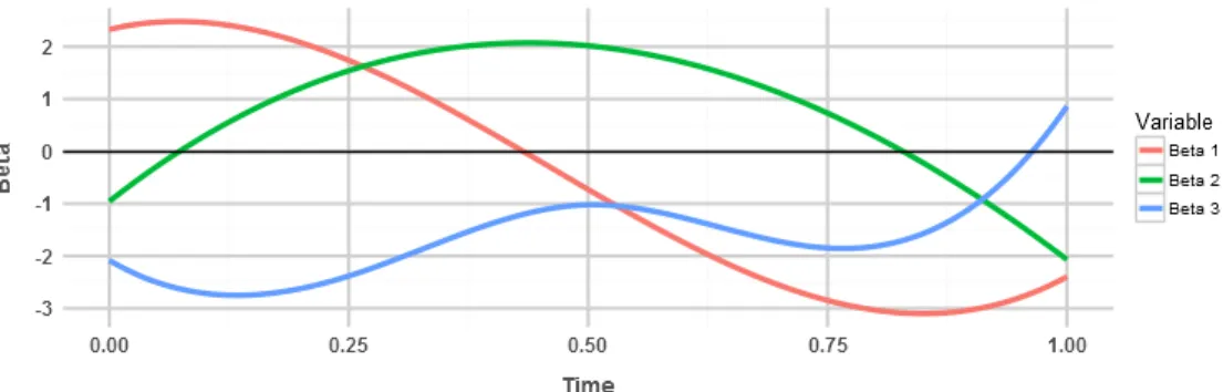
In this section, we observe the performance of the proposed time-varying bias corrected ridge inference procedure through simulation studies. We first generate an n×p design matrix using n i.i.d. rows from Np(0, I), withn = 300 andp∈ {300,500}. The time-varying coefficient vectors β(t) are set up such that there are s = 3 non-zero elements and p−3 zeros for all t ∈ [0,1]. These non-zero elements in β(t) are generated by sampling nodes from a uniform distribution U(−b, b) at regular time points and smoothly interpolating on the interval [0,1] using cubic splines.

Figure 2.2: Simulated non-zeroβ(t) withb= 2.5 We simulated several sets of stationary error processes:

1. ei are i.i.d. Nn(0, I).

2. ei is an AR(1) processei =ϕei−1+i whereϕ= 0.7 andi are i.i.d. Nn(0, I). 3. ei are i.i.d. Student’st(3)/

√ 3.

The remaining parameters include the kernel bandwidthbn= 0.1,λ1 =

p

2 log(p)/n, λ2 = 1/n, andζ= 0.

(25)

For individual testing H0 : βj = 0 at time t, we reject the null hypothesis at significance level α if

the corresponding raw p-value ˜Pj,t ≤ α. Using the framework above with an empty active set S = ∅

demonstrates a<5% nominal type I error rate, albeit conservatively.

Figure 2.3: Raw p-values under Null

For multiple testing H0 :βj = 0, j∈Gat timet, we reject the null hypothesis at significance levelαif

the corresponding multiplicity-adjusted p-value Pj,t ≤α. Therefore, our proposed method’s false positive (FP) rate over the intervalB= [bn,1−bn] is written as

1 n(1−bn)(p−s) X j∈Sc X t∈B P(Pj,t≤α) (2.29)

and the false negative (FN) rate is written as 1 n(1−bn)s X j∈S X t∈B P(Pj,t> α) (2.30) The familywise error rate (FWER) in our simulation setup is defined as the proportion of multiplicity-adjusted tests with at least 1 type I error.

FWER = 1 n(1−bn) X t∈B P   \ j∈Sc {Pj,t|Pj,t≤α} 6=∅   (2.31)

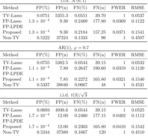
For each simulation setup, we report the false positive counts and rates, false negative counts and rates, family-wise error rates, and root mean square errors (RMSE) of β. These examples are high-dimensional since we havens(1−bn) = 720 nonzero parameters and a sample size of 300. We compared the performance of the proposed method against the following procedures:

(26)

1. (TV-Lasso) - The time-varying Lasso, an adaptation of the standard LASSO to the kernel smoothing environment with bn = 0.1 andλ1 selected using cross validation. (Generally on the order of 1.5×

p

2 log(p)/n)

2. (FP-Lasso) - The false-positive Lasso, whereλ1is tuned to match the type I error rate of the proposed

method. (Generally on the order of 5×p

2 log(p)/n). This allows us to compare power at similar levels of individual and family-wise errors. In practice, such precise tuning of λ1 on type I errors would be

impossible since the active setS is unknown, making FP-Lasso “pseudo-oracle.”

3. (FP-LPDE) - An adaptation of the de-biased LASSO [Zhang and Zhang, 2014] inference procedure with the estimator

ˆ

βDeBias(t) = ˆβLasso(t)+(nbn)−1MtXt>(Yt−XtβˆLasso(t)), where the multiplicity-adjusted significance levelαis selected to yield identical type I error rates as the proposed method. Also “pseudo-oracle”. 4. (Non-TV) - The original non-time-varying method of [B¨uhlmann, 2013] which ignores the dynamic

(27)

Our results are shown in Tables 2.5 and 2.5, with 20 replications for each setting. i.i.d. N(0,1)

Method FP(%) FP(n) FN(%) FN(n) FWER RMSE

TV-Lasso 0.0751 5355.3 0.0551 39.70 1 0.0537 FP-Lasso 1.3×10−4 9.30 0.2469 177.80 0.0369 0.1122 FP-LPDE Proposed 1.3×10−4 _9.30 _0.2184 _157.25 _0.0371 _0.1541 Non-TV 0.5222 37224 0.1333 96 1 0.4507 AR(1), ϕ= 0.7

TV-Lasso 0.0755 5382.5 0.0544 39.15 1 0.0532 FP-Lasso 1.1×10−4 _7.80 _0.2647 _190.60 _0.0319 _0.1120 FP-LPDE Proposed 1.1×10−4 _7.85 _0.2272 _165.80 _0.0321 _0.1546 Non-TV 0.5337 38040 0.0667 48 1 0.4531 i.i.d. t(3)/√3

TV-Lasso 0.0693 4938.6 0.0544 39.15 1 0.0525

FP-Lasso 1.7×10−4 _12.00 _0.2460 _177.15 _0.0402 _0.1112

FP-LPDE

Proposed 1.7×10−4 12.00 0.2303 165.80 0.0410 0.1542

Non-TV 0.5244 37380 0.1667 120 1 0.4510

(28)

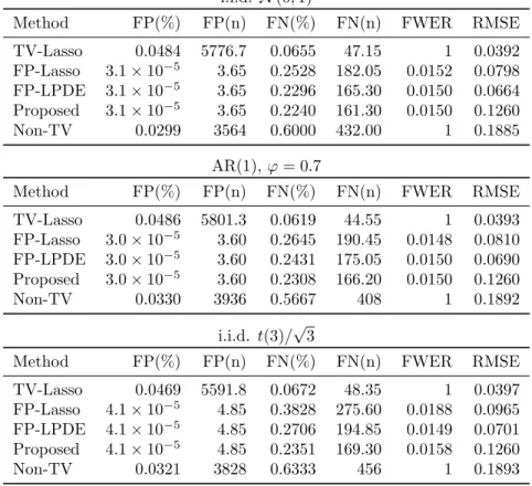
i.i.d. N(0,1)

TV-Lasso 0.0484 5776.7 0.0655 47.15 1 0.0392 FP-Lasso 3.1×10−5 _3.65 _0.2528 _182.05 _0.0152 _0.0798 FP-LPDE 3.1×10−5 3.65 0.2296 165.30 0.0150 0.0664 Proposed 3.1×10−5 3.65 0.2240 161.30 0.0150 0.1260 Non-TV 0.0299 3564 0.6000 432.00 1 0.1885 AR(1), ϕ= 0.7

TV-Lasso 0.0486 5801.3 0.0619 44.55 1 0.0393 FP-Lasso 3.0×10−5 _3.60 _0.2645 _190.45 _0.0148 _0.0810 FP-LPDE 3.0×10−5 _3.60 _0.2431 _175.05 _0.0150 _0.0690 Proposed 3.0×10−5 _3.60 _0.2308 _166.20 _0.0150 _0.1260 Non-TV 0.0330 3936 0.5667 408 1 0.1892 i.i.d. t(3)/√3

TV-Lasso 0.0469 5591.8 0.0672 48.35 1 0.0397

FP-Lasso 4.1×10−5 _4.85 _0.3828 _275.60 _0.0188 _0.0965

FP-LPDE 4.1×10−5 _4.85 _0.2706 _194.85 _0.0149 _0.0701

Proposed 4.1×10−5 _4.85 _0.2351 _169.30 _0.0158 _0.1260

Non-TV 0.0321 3828 0.6333 456 1 0.1893

Table 2.2: Simulation results for the case ofn= 300, p= 500, s= 3, b= 2.5.

Empirically, we see that family-wise error control is not maintained in the non-time-varying case using [B¨uhlmann, 2013], since it’s unable to accommodate the flip-flopping nature ofβ(t). The proposed method does maintain FWER control in all simulation setups, but is conservative in the case ofp= 500. This FWER control naturally demands a very small false positive rate, whereas the time-varying Lasso has much greater false positive rates due to the the bias froml1 regularization.

We also observe that the proposed method fares worse in terms of RMSE than the other time-varying methods. This is largely due to fixing λ2 to be small in order to circumvent complications surrounding

parameter tuning such as cross validation and to make the problem more amenable to the conditions of 2.1. Due to the bounds on Varβj(t)ˆ , minimizing RMSE is likely to be sub-optimal for detection, in terms of λ2selection.

(29)

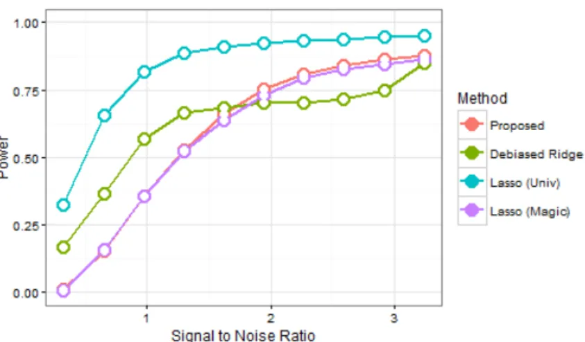
At similar type I error levels, the proposed time-varying de-biased ridge method yields greater detection power in all simulation setups. De-biasing the Lasso helps bring the two methods closer in terms of power, but comes at the expense of substantially increased complexity and computation time. The simulations were performed using an Intel i5-4970K running R 3.2.2 for Windows with Intel MKL linear algebra libraries.

Method Runtime

TV-Lasso 1

FP-Lasso 19

FP-LPDE 1445

Proposed (raw p-values only) 9 Proposed (adjusted p-values) 26

Non-TV <1

Table 2.3: Time to run 20 replications, in minutes. p= 500 withN(0,1) i.i.d. errors

The Lasso and De-Biased Lasso are based on code from glmnet and SSLasso by J. Friedman and A. Javanmard, respectively [Friedman et al., 2010a][Javanmard and Montanari, 2014]. The reported run times for FP-Lasso and FP-LPDE includes time spent on divide and conquerλ1andαsearches for FPR matching.

The additional computation time is quite substantial in the former case and negligible in the latter. The time-varying methods above are bottle-necked by estimation of the covariances ofX within local bandwidths, which we attempt to remedy in Chapter 3 using structure decomposition.

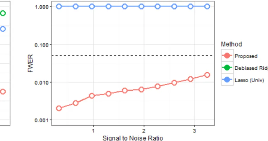
By varying the signal magnitude scalar bfrom 0.25 to 2.5, we can examine the behavior of the proposed method and its FWER control at various signal-to-noise ratios (S/N).

(30)

Figure 2.6: Power vs S/N

The proposed method maintains FWER control across the spectrum of signal-to-noise ratios examined above, although of course the power suffers at lower signal-to-noise ratios.

2.6 Real Data Example - Learning Brain Connectivity

We illustrate our proposed method with a problem about estimating functional brain connectivity in patients from a Parkinson’s disease study. The principle of functionally segregated brain organization in humans is well established in imaging neuroscience, and connectivity is understood as a network of statistical depen-dencies between different regions of the nervous system.

Slowly time-varying graphs have strong implications in modeling brain connectivity networks using resting state functional magnetic resonance imaging (fMRI) data. Traditional correlation analysis of resting state blood-oxygen-level-dependent (BOLD) signals of the brain show considerable temporal variation on small timescales [CITE], and many treatments for Parkinson’s disease are evaluated by medical professionals based on changes to a subject’s connectivity network. For example, patients with Parkinson’s disease generally have increased connectivity in the primary motor cortex, especially during “off state” times. [CITE]

Furthermore, in view of the high spatial resolution of fMRI data, brain networks of subjects at rest are believed to be structurally homogeneous with subtle fluctuations in some, but a small number, of connectivity edges [CITE]. Therefore, a popular approach to learn brain connectivity is the node-wise regression network (i.e. the neighborhood selection procedure), where the time-varying coefficients represent dynamic features of the corresponding edges. We do remark, however, that the neighborhood selection approach we adopt in this

(31)

example is merely an approximation of the full multivariate distributions due to ignoring correlation among node-wise responses. This may lead to some power loss in finite samples, but is asymptotically equivalent in terms of variable selection.

Our real data example uses fMRI data collected from a study of patients with Parkinson’s disease (PD) and their respective normal controls. PD is typically characterized by deviations in functional connectivity between various regions of the brain. Additionally, resting state functional connectivity has been shown as a candidate biomarker for PD progression and treatment, where more advanced stages or manifestations of PD are associated with greater deviations from normal connectivity. Each resting state data matrix in our example contains 240 time points and 52 brain regions of interest (ROI). The time points are evenly sampled and the time indices are normalized to [0,1]. Previous study of this dataset showed that the temporal and spatial connectivity patterns differ significantly between PD and control subjects [Liu et al., 2014].

The brain connectivity network is constructed using the neighborhood selection procedure. In essence, it is a sequence of time-varying linear regressions by enumerating each ROI as the response variable and sparsely regressing on all the other ROIs. Since fMRI data was collected from subjects at rest rather than subjects assigned specific tasks at certain times, we did not pool the data across subjects for analysis.

(32)

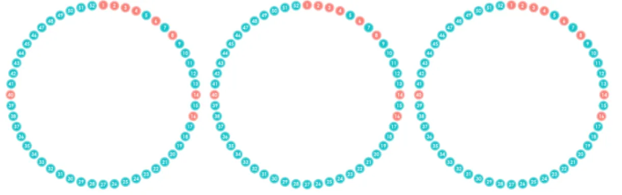
Figure 2.7: Connectivity Network in Control Subject aroundt= 0.25

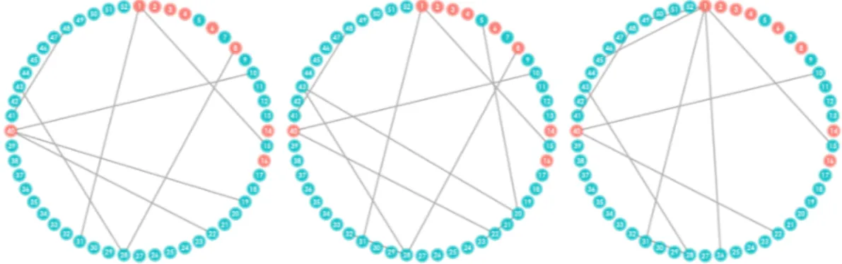
Figure 2.8: Connectivity Network in Parkinson’s Subject aroundt= 0.25

In the examples above, we plot the connectivity networks of one healthy and one Parkinson’s diagnosed patient for 3 sequential time points surroundingt= 0.25. Regions of the brain known to be associated with motor control are highlighted using red nodes. In contrast, blue nodes designate areas of the brain either known to be unrelated to motor control or whose functions in humans are not well understood. Different patterns of connectivity in the networks can be found by comparing the PD and control subjects. From the graphs, we can observe the slow change in the networks over time. Most edges are preserved on a small timescale, but there are a few number of edges changing. For instance in the PD subject, ROI 01 → 40 is unconnected in the first time point but is connected in the second and remains connected in the third. Generally, when there is substantial activity to study, we tend to observe a more diverse set of edges in healthy subjects and greater connectivity involving the motor-related regions in PD subjects.

(33)

Figure 2.9: Connectivity Network in Control Subject aroundt= 0.80

Figure 2.10: Connectivity Network in Parkinson’s Subject around t= 0.50

There are also times when, due to the nature of stringent FWER control and variable selection process, that the estimated connectivity networks may be exceptionally sparse or empty. This serves to reinforce the importance of the time-varying design, particularly for resting state data, since traditional methods which don’t study temporal variations have less power to detect differences between subjects when the signals only manifest for short periods of time.

(34)

Chapter 3

Kronecker Structured Covariance

Estimation

3.1 Introduction

There has been much recent interest in the estimation of sparse graphical models in the high-dimensional setting for ann×pGaussian matrixX, where the observationsx1, ...,xn are i.i.d. N(µ,Σ),µ∈Rp, andΣ

is a positive definitep×pmatrix. A graphical model can be built by using the variables or features as nodes and by using non-zero elements of the precision or inverse covariance matrixΩ =Σ−1 as edges such that nodes representing featuresi, jare connected if Ωij6= 0. The zeroes in Ω correspond to no connecting edge, indicating that the pair of variables are conditionally independent of each other, given the other variables in X[Lauritzen, 1996]. These models see applications in various fields such as meteorology, communications, and genomics. For example, graphical models are frequently used in gene expression analysis to study patterns of association between different genes and create therapies targeting these pathways.

The classical method of estimating the covariance matrix Σis the sample covariance matrix:

ˆ S= 1

n−1X

>_X _(3.1)

While the sample covariance matrix is an unbiased estimator of the true covariance matrix, it suffers from high variance in a high-dimensional setting wheren < p. Furthermore, the resulting matrix is singular and incompatible with problems whereΩ=Σ−1 _{is the parameter of interest. Alternatively, a low rank}

approx-imation is sometimes used where we take the rgreatest principle components from an eigendecomposition of ˆS. ˆ SP CA= r X i=1 σ2_iviv_i> (3.2)

(35)

minimization problem [Eckart and Young, 1936].

arg min

S∈S++,rank(S)≤r

|Sˆ−S|2F (3.3)

However, the PCA estimator yields substantial bias in the high-dimensional setting. [Lee et al., 2010] [Rao et al., 2008]

The maximum likelihood approach is a direct estimation method where the precision matrix estimator ˆ

ΩM LE is obtained by maximizing the likelihood with respect toΣ−1_{, and explained in more detail in the}

Graphical Lasso section below. For the purpose of graphical models, however, the maximum likelihood precision matrix estimator lacks interpretability and yields high variance in a high-dimensional setting. Specifically, ΩM LEˆ will not have any elements which are exactly zero. Consequently, graphs constructed using ˆΩM LE would not be useful for identifying conditional independence between pairs of variables since edges exist between all pairs of nodes.

Thus arises a need for the estimation of a sparse dependence structure where many elements of the inverse covariance matrix estimator are set to zero. This literature advocating sparse estimation of covariance and inverse covariance matrices can be traced back to [Dempster, 1972]. An early approach to achieving a sparse estimator is the backwards selection method, where the least significant edges are sequentially removed from a fully connected graph until the remaining edges are all significant according to partial correlation tests. The backwards selection method did not take multiple testing into consideration, although [Drton and Perlman, 2007] later proposed a conservative procedure which did.

More recent work in graphical model estimation involves nodewise regression procedures similar to the Parkinson’s data example from Chapter 1. [Meinshausen and B¨uhlman, 2006] proposed regressing each vari-able on all the other varivari-ables using `1 penalized regression, with graph edges representing the significant

regression results. [Zhou et al., 2009] further extended the method to other variants of penalized regression such as the adaptive LASSO. These nodewise regression methods are able to consistently recover the support ofΩto produce a directed graphical model but cannot estimate the elements of Ωthemselves.

A maximum likelihood approach with the `1penalty was studied by [Yuan and Lin, 2007],

[Banerjee et al., 2008], [Friedman et al., 2010b], and [d’Aspr´emont et al., 2008]. These approaches were later generalized to the smoothly clipped absolute deviation (SCAD) penalty [Fan et al., 2009], [Lam and Fan, 2009].

This chapter explores the algorithms, properties, and performance of Kronecker graphical lasso (KGLasso) methods for the purposes of constructing Gaussian graphical models and the estimation of Kronecker decompose-able covariance and precision matrices. We begin with ordinary KGLasso [Tsiligkaridis, 2014],

(36)

followed by our extension to the joint Kronecker graphical lasso (JKGLasso) case for the estimation of covariance matrices across different groups of subjects.

3.1.1 Notation

DenoteIpto be thep×pidentity matrix and1pa vector of lengthpwith all entries equal to 1. Define vec to be the matrix vectorization function inRp×q→Rpq such that vec(M) is the vectorized form ofM obtained

by concatenating the columns ofM. For higher tensor spaces, let vec :Rp1×...×pK _→

Rp1...pK _{be the tensor} vectorization function where we concatenate via the array dimensions in reverse order beginning with K. LetS(·) denote the soft thresholding operatorS:_R2_→

R1 such thatS(x, c) = sign(x) max(|x| −c,0)

Define |M|1 to be the L1 norm of a matrix M. Define |M|F to be the Frobenius norm of a matrix M. Define Sp ₌ _{M _∈

Rp×p : M =M>} to be the set of p×p symmetric matrices, and let S+p denote the

set of symmetric positive definite matrices and Sp₊₊ the set of symmetric semi-positive definite matrices. Denote Mij and (M)ij to be the (i, j)-th element in matrix M where i, j ∈ N1. DefineMIJ and (M)IJ,

I ∈Np1_{, J} _∈

Np2 _{to be the sub-matrix of} _M _{corresponding to the (i, j)-th elements in} _M _{such that}_i _∈_I

andj∈J.

For a sequence of positive real numbers{an}n∈_Nand random variables{Xn}n∈_Non space (Ω,F, P), define Xn =OP(1) to say that Xn is stochastically bounded: ∀ > 0,∃M > 0 such that P(|Xn| > M)< ∀n. DefineXn=OP(an) to say X_ann =OP(1).

3.1.2 The Graphical Lasso

Given a set ofni.i.d. multivariate Gaussian observations{xj}n

j=1, xj∈R

p_{with mean zero (without loss of} generality), positive definite covariance matrix Σ∈S++p , and sample covariance matrix ˆS= n1

Pn

j=1xjx>j, then the log-likelihoodl(Σ) is written

l(Σ) = log det(Σ−1)−tr(Σ−1S)ˆ (3.4)

The late 2000’s saw an interest in `1-regularized maximum likelihood estimators [Banerjee et al., 2008]

(37)

and are obtained by solving the`1-regularized minimization problem ˆ Σ= arg min Σ∈Sp₊₊−l(Σ) +λ|Σ −1 |1 (3.5) = arg min Σ∈Sp ++ tr(ˆSΣ−1)−log det Σ−1 +λ|Σ−1_| 1 (3.6)

where λ ≥ 0 is a tuning parameter. [Friedman et al., 2010a] introduced an iterative algorithm using block coordinate descent to obtain the GLasso estimators inO(p4_{) time, and}_O(p3_{) in the sparse case. An}

alternative algorithm was introduced by [Hsieh et al., 2011] with the same computational complexity. [Rothman et al., 2008] and [Zhou et al., 2010] showed the high dimensional consistency in Frobenius norm of the GLasso estimators for an appropriate choice ofλ

kΣˆ−1−Σ−1kF =OP r (p+s) log(p) n ! (3.7)

where ˆΣis the GLasso estimator andsis a measure of sparsity denoting an upper bound on the number of nonzero off-diagonal entries inΣ−1

3.2 The Kronecker Covariance Framework

We consider the Kronecker covariance model:

Σ=A⊗B (3.8)

Where Σ is thep×pcovariance matrix for the observed data and Aand Bare pA×pA andpB×pB positive definite matrices, respectively, such thatpApB =p. This type of low-dimensional Kronecker covari-ance matrix representation can be found in communications to model signal propagation from systems with multiple input multiple output (MIMO) radio antenna arrays such as modern home wi-fi routers [Werner and Jansson, 2007][Werner et al., 2008], in genomics to estimate correlations between genes and their associated factors [Yin and Li, 2012], facial recognition [Zhang and Schneider, 2010], recommendation systems, and missing data imputation [Allen and Tibshirani, 2010]. Typically, the motivation behind using the Kronecker model is the pursuit of computational and mathematical tractability or a very low dimensional representation given the model assumptions.

(38)

not unique, since each is identifiable only up to a constant. This is true of the methods introduced in this chapter, although the resulting estimator forΣ=A⊗B is unique.

[Allen and Tibshirani, 2010] referred to this model as a transpose-able model, where both the rows and columns are considered to be features of interest. Transpose-able models and the Kronecker covariance model are special cases of the matrix variate normal distribution from [Efron, 2009], where separate covariance matrices are used for the rows and columns. The authors provided a concept of a movie recommendation engine which used this model such that the relationship between Customer A’s rating of Movie 1 and Customer B’s rating of Movie 2 is modeled using the interaction between Customers A and B, and Movies 1 and 2.

Generally speaking, the simple Kronecker product covariance structure follows when we have a data matrixX∈Rn×p with row means v∈Rn, column meansu∈Rp, row covariance A∈Rn×n, and column

covarianceB∈Rp×p. By vectorizing the data matrixX, we have

vec(X)∼ N vec(v1>_p +1nu>),A⊗B

(3.9)

where1k is a vector of lengthkwith all entries equal to 1. Therefore, an elementXij inXis distributed Xij ∼ N(vi+uj, σij) and follows a mixed effects model without an assumption of independence between errors from the rows and columns.

The model can be readily extended beyond 2 dimensional arrays for Xusing appropriate vectorization. [Flaxman et al., 2015] and [Bonilla et al., 2008] compared the Kronecker covariance structure to tensor Gaus-sian products.

3.3 The Kronecker Graphical Lasso for One Group

Suppose we haveni.i.d. observations from a multivariate Gaussian distribution with mean zero and covari-anceΣ=A⊗BwhereA∈SpA

++,B∈S

pB

++ then the`1-penalized maximum likelihood estimator is obtained

by solving ˆ Σ= arg min Σ∈Sp ++ tr(ˆSΣ−1)−log det Σ−1 +λ|Σ−1_| 1 (3.10) = arg min Σ∈Sp ++

trhS(Aˆ −1⊗B−1)i−pBlog det A−1

−pAlog det B−1

+λ|A−1_|

(39)

where λ≥ 0 is a regularization parameter. When Aor B is fixed in the objective minimization function above, then the function is convex with respect to the other argument [Tsiligkaridis and Hero, 2013]. There-fore, we consider an alternating or “flip-flop” approach to handling the dual problem of fixing one half of the Kronecker covariance matrix and optimizing over the other half.

The original penalized flip-flop (FFP) algorithm introduced by [Tsiligkaridis, 2014] and [Allen and Tibshirani, 2010] is given below. Both minimization steps are solved using GLasso.

Flip Flop Algorithm for KGLasso

Input ˆS, λ >0, >0 Initialize ˆΣ−1₌_I p andA−1∈S pA ++ repeat ˆ Σ−1 prev←Σˆ−1 TA← 1 pA PpA i,j=1A −1 i,jSj,iˆ λA← λ|A−1|1 pA B−1←arg min_B_∈SpB ++

tr(B−1TA)−log det B−1+λA|B−1_| 1 TB ← 1 pB PpB i,j=1B −1 i,jSj,iˆ λB ←λ|B−1|1 pB A−1_←_{arg min} A∈SpA₊₊ tr(A−1_T B)−log det A−1 +λB|A−1_| 1 ˆ Σ−1_←_A−1_⊗_B−1 untilkΣˆ−1₋_Σˆ−1 prevk ≤

The flip flop algorithm for KGLasso has complexity inO(p4

A+p4B) compared to GLasso’sO(p4Ap4B).

3.3.1 Simulation Results

We consider moderately sparse covariance matricesΣwith dimensionp= 400, decompose-able into smaller matricesΣ=A⊗Bwith dimensionspA=pB= 20. We constructA,Bfrom different distributions including a block Toeplitz structure whose block structure is likely to favor the Kronecker product representation, and a more general structure based on a positive definite Erdös - Rényi graph [Erdös and Rényi, 1960]. A visualization of the latter is given below, where greys represent zeros, lighter shades represent more positive values, and darker shades represent more negative values.

(40)

Figure 3.1: A covariance map and graph ofA

Figure 3.2: A covariance map and graph ofB

(41)

Figure 3.3: A covariance map and graph ofΣ=A⊗B

We compared the performance of 4 different methods: The KGLasso, the na¨ıve GLasso without con-sideration of the Kronecker covariance structure, the non-sparsified KGLasso based on the flip flop al-gorithm of the corresponding un-penalized maximum likelihood, and the CLIME by [Cai et al., 2011]. We evaluated the performance using Frobenius norm losses on the covariance and precision matrices for n ∈ {10,25,50,100,200,400,800,1000}, and the tuning parameter λwas chosen experimentally and sepa-rately for each method to minimize Frobenius norm loss on the covariance matrix (Usually close toλ= 0.4). In the case of CLIME, λ was selected automatically using the fastclimepackage in R and its precision matrix estimator was further thresholded below to promote sparsity. The threshold cutoff was selected ex-perimentally to minimize Frobenius norm loss on the covariance matrix. 100 trials were run for each method for each value ofn.

Inference of high-dimensional linear models with time-varying coefficients