Gazing at Cirrus Clouds for 25 Years through a Split Window. Part I: Methodology
ANDREWK. HEIDINGER ANDMICHAELJ. PAVOLONIS
NOAA/NESDIS Center for Satellite Applications and Research, Madison, Wisconsin
(Manuscript received 26 September 2007, in final form 22 August 2008) ABSTRACT
This paper demonstrates that the split-window approach for estimating cloud properties can improve upon the methods commonly used for generating cloud temperature and emissivity climatologies from satellite imagers. Because the split-window method provides cloud properties that are consistent for day and night, it is ideally suited for the generation of a cloud climatology from the Advanced Very High Resolution Radio-meter (AVHRR), which provides sampling roughly four times per day. While the split-window approach is applicable to all clouds, this paper focuses on its application to cirrus (high semitransparent ice clouds), where this approach is most powerful. An optimal estimation framework is used to extract estimates of cloud temperature, cloud emissivity, and cloud microphysics from the AVHRR split-window observations. The performance of the split-window approach is illustrated through the diagnostic quantities generated by the optimal estimation approach. An objective assessment of the performance of the algorithm cloud products from the recently launched space lidar [Cloud-Aerosol Lidar and Infrared Pathfinder Satellite Observation/ Cloud-Aerosol Lidar with Orthogonal Polarization (CALIPSO/CALIOP)] is used to characterize the per-formance of the AVHRR results and also to provide the constraints needed for the optimal estimation approach.
1. Introduction
As the data record from the National Oceanic and Atmospheric Administration’s (NOAA) Advanced Very High Resolution Radiometer (AVHRR) approaches 30 years in length, its relevance as a dataset for studying multidecadal climate variability grows. In particular, the AVHRR has proven capable of producing useful in-formation on global cloudiness. This paper explores a new application of an old approach for the generation of a global multidecadal cloud climatology: the split-window method. The cloud properties of interest here are the cloud-top temperature Tc, the cloud 11-mm infrared emissivity ec, and a measure of cloud microphysics,
de-noted here asb.The application of this approach is de-signed for a new version of the AVHRR Pathfinder At-mospheres Extended dataset (PATMOS-x), which is an extension in terms of algorithms, products, and temporal coverage of the PATMOS data described by Jacobowitz et al. (2003) and Stowe et al. (2002). This effort represents
the first global and multidecadal application of the split-window algorithm. This algorithm is also run operation-ally within the NOAA National Environmental Satellite, Data, and Information Service (NESDIS) as parts of the Clouds from AVHRR Extended (CLAVR-x) processing system.
As indicated by the title, the focus of this paper is on cirrus clouds that are defined as semitransparent ice clouds. The split-window approach is certainly appli-cable to other clouds and is applied to all clouds in PATMOS-x. Because of the higher opacity of most lower-level clouds and the reduced temperature con-trast with the surface, the behavior of the split-window approach implemented in the one-dimensional varia-tional data assimilation (1DVAR) analysis in the pres-ence of low-level clouds is more similar to that from a channel IR approach. The performance of single-channel IR approaches forTcestimation has been well
documented (Nieman et al. 1993). The technique for determining cloud type and phase for each AVHRR cloudy pixel is given by Pavolonis et al. (2005). This typing algorithm classifies cloudy pixels as being fog, water, supercooled water, cirrus, multilayer, or opaque ice cloud. The fog, water, and supercooled water types are treated as water phase clouds and the others are
Corresponding author address: Andrew Heidinger, NOAA/ NESDIS Center for Satellite Applications and Research, 1225 West Dayton St., Madison, WI 53705.
E-mail: [email protected] DOI: 10.1175/2008JAMC1882.1
treated as ice phase clouds. The cirrus type is meant to refer to semitransparent single-layer ice clouds. The multilayer cloud type is dominated by cirrus cloud over-laying lower water clouds. The opaque ice cloud type consists of opticaly thick high-level ice clouds.
The goal for this algorithm is to generate climate data records of Tc, ec, and b over the three decades of
AVHRR observations. To be relevant, the cloud clima-tology from PATMOS-x must add to the information provided by the most used and successful satellite cloud climatology, the International Satellite Cloud Clima-tology Project (ISCCP) (Rossow and Schiffer 1999). During the day, ISCCP uses the visible (VIS)/IR ap-proach for cloud property estimation by estimatingec
using an optical depth retrieval performed at 0.63mm (VIS) and using the value ofecto estimateTcfrom the
11-mm (IR) radiance. During the night, only the IR radiance is used. These approaches perform very dif-ferently for optically thin cloud. The main benefit of the split-window approach relative to the ISCCP ap-proach is that it delivers consistent performance for all solar illumination conditions (including night) and offers an improvement to the ISCCP IR-only nighttime results for optically thin cirrus. Last, the split-window method provides a measure of cloud microphysics that is absent from the ISCCP methodology. While PATMOS-x does not offer the eight times per day sampling of ISCCP, it does provide four times per day sampling (since 1992) with an approach that should offer consistent results at all times of day. Part II of this series will analyze the merits of the climatology derived from the split-window approach as described here.
With the launch of the Geoscience Laser Altimeter System (GLAS) on the Ice, Cloud and Land Elevation Satellite (ICESAT) in 2003 and the Cloud-Aerosol Lidar with Orthogonal Polarization (CALIOP) on the Cloud-Aerosol Lidar and Infrared Pathfinder Satellite Ob-servation (CALIPSO) mission in 2006, the National Aeronautics and Space Administration (NASA) has pro-vided unprecedented information on the vertical profiles of cloudiness that can be used to characterize the per-formance from passive sensors such as the AVHRR. Be-cause of the orbit of CALIPSO, it provided much more collocated data with the AVHRR on NOAA-18 and only data from CALIPSO will be used here. ICESAT does provide additional AVHRR collocation opportu-nities with the NOAA polar-orbiting satellites in morn-ing orbits and we intend to extend this analysis usmorn-ing ICESAT in the future. Another reason to use CALIPSO is that it flies in formation with the Moderate Resolution Imaging Spectroradiometer (MODIS) and other Earth Observing System (EOS) sensors. Hence, the current period represents a golden age of polar-orbiting satellite
cloud remote sensing and we are fortunate that the AVHRR record extends into it. One major goal of this paper is to quantify the performance of the AVHRR relative to these superior observing systems. These re-sults can then be used to determine the confidence of the cloud variability observed over the past three de-cades by the AVHRR.
This paper is divided into several sections: section 2 describes the physics of the split-window approach. The datasets used in this analysis are described in section 3 and the retrieval methodology is presented in section 4. The procedure used to generate the error estimates for the retrieval is given in section 5 and the estimates of the forward model error are described in section 6. An ex-ample of the application of the split-window approach to one scene is given in section 7. Section 8 provides a quantitative comparison of the split-window results relative to those from MODIS and CALIPSO. Section 9 describes the accuracy of the high-cloud amounts gen-erated from the split-window method. Last, section 10 provides our conclusions and plans for future research.
2. The split-window method
While the split-window observations on the AVHRR were originally included for sea surface temperature estimation, their use for the generation of cloud prop-erties commenced early in the life of the AVHRR data record. One of the earliest descriptions of the use of split-window observations for the estimation ofTcandec
is given by Inoue (1985). Inoue (1985) estimatedTcand
ecby assuming a fixed value ofb51.08. This value was
determined through analysis of several AVHRR scenes recorded over the western Pacific Ocean. Inoue found that the use of fixed value of b allowed for accurate determination ofTcwhenec.0.4. A rigorous study of
the behavior of the split-window observations in the presence of cirrus clouds was given by Parol et al. (1991). Determination ofbfrom analysis of theT11–T12curves
from scenes over Europe was performed by Giraud et al. (1997). The more recent study of Cooper et al. (2003) explored the use of split-window measurements for es-timatingTc,ec, and particle size when cloud boundary
information is provided by an active sensor such as a lidar and a radar. A similar study applied to contrails was conducted by Duda and Spinhirne (1996) using aircraft-based lidar and radiometer observations.
The split-window method derives cloud properties from two spectrally separated measurements within the 8–13-mm infrared region. For application to the AVHRR, the measurements used are the 11-mm (T11)
and the 12-mm (T12) brightness temperatures. For a
split-window observations are the cloud temperatureTc,
the cloud emissivityec, and the cloud microphysics. As is
commonly done in research involving split-window ob-servations, the cloud microphysics are represented by the parameterb, defined as
b5ln(1 ec,12) ln(1 ec,11)
, (1)
whereec,11andec,12are the cloud emissivities at 11 and
12 mm (Inoue 1985); b is a strong function of cloud particle size and phase. Figure 1 shows the variation ofb computed from Mie theory for ice and water droplets and from bulk nonspherical ice scattering models of Baum et al. (2005). In general for both ice and water clouds, larger values of bimply smaller particles. The values ofbin Fig. 1 are computed solely from the single scattering properties using the method given in Parol et al. (1991). The kink in the Baum curve arises from the discrete variation in habit mixture as particle size varies. As this figures illustrates,bcan be used as a surrogate for cloud particle size, thoughbloses sensitivity to size for particles larger than 30mm in radius. A fundamental radiometric measure of cloud microphysics is provided bybthat is available day and night and does not require any a priori assumptions on particle size, shape, or dis-tribution.
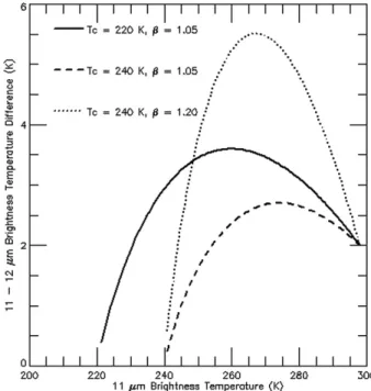
Figure 2 demonstrates the relationship betweenTc,ec,
and b on the split-window observations. This figure shows the variation ofT11andT11–T12for three sets of
values of Tc and b characteristic of ice clouds. The
curves are computed by varying ecfrom 0 to 1. For a
given value ofTcandec,T11–T12increases asbincreases.
As Fig. 2 shows, measurements of T11 andT11–T12are
not sufficient for a unique estimate of Tc, ec, and b.
However, Tc,ec, andb do not constitute three
inde-pendent pieces of information. Given a value ofTc,ec
andbare determined directly from the 11- and 12-mm radiative transfer equations. Therefore the information content is fundamentally fromTcand the spectral
vari-ation ofec;bis a suitable metric of this spectral variation
ofecbecause it offers a direct link to the microphysics as
shown by Fig. 1 and can be derived from the two split-window channels. Uniqueness is not the main limitation of the split-window approach. The main weakness is the inherent lack of sensitivity of the split-window observa-tions toTcfor optically thin clouds; this is discussed in
sections 7 and 8.
It is important to note that the observations used here have a spatial resolution of 1–4 km and therefore may be composed of pixels that are not completely cloudy. In infrared remote sensing, the observed emissivities are actually the product of the true emissivities and subpixel cloud fraction. In infrared remote sensing literature, this product is often referred to as the effective cloud amount (Menzel et al. 2008). Figure 3 demonstrates the sensitivity of estimating bin the presence of partially cloudy observations when the pixels are assumed to be completely cloud covered, as done in our retrieval ap-proach. The curves in Fig. 3 were generated by multi-plying each emissivity in Eq. (1) by the subpixel cloud FIG. 1. Variation inbas a function of the cloud particle effective
radius using the ice scattering properties reported by Baum et al. (2005) and from Mie theory.
FIG. 2. Variation inT11–T12withT11simulated for cirrus cloud
over a surface with a temperature of 300 K. Each curve corre-sponds to different values of cloud temperature (Tc) andb. Each curve is generated by varyingecfrom near zero to unity holdingb andTcconstant.
fraction. Each curve was computed assuming a fixed value ofec,11(cloud emissivity) and a true value ofb51.0. As
this figure shows, the estimated b always decreases as the cloud fraction falls below 1.0. The effect is larger for larger emissivities. Therefore, this effect is largest for optically thick cloud with small subpixel cloud amounts. Because this paper deals with cirrus that are optically thin and are typically spatially extensive, we are confident that the impact of subpixel cloudiness on our retrievedbvalues is small. While this effect may be sig-nificant when using sounder data that typically have much larger pixel sizes, the pixel sizes employed here should be adequate to allow us to assume fully cloud-filled pixels. In addition, the AVHRR processing em-ployed here screens all pixels that occur on cloud edges, which should also mitigate this effect. For the remainder of this paper, we will assume all pixels are completely cloud covered and that the cloud emissivity variations are not due to subpixel cloud fraction variations.
3. Generation of CALIPSO, MODIS, and AVHRR comparisons
The main analysis approach used in this paper is the generation of simultaneous collocated comparisons between the AVHRR onNOAA-18and MODIS and CALIPSO data from the EOS A-train. CALIPSO will provide vertical profiles of cloud extinction and cloud phase. At the date of the submission of this paper, the only available CALIPSO products were profiles of cloud layers and midlayer cloud temperatures (Vaughan et al. 2004). In addition to the midlayer temperatures, the cloud-top temperatures Tc and pressures Pc were
es-timated from the cloud-top altitudes and the atmo-spheric profiles in the level-1 CALIPSO data. At the time this study was done, the opacity and phase infor-mation was not yet available and the CALIPSO prod-ucts used here were currently listed as provisional. Even with these limitations, we contend that the CALIPSO data provide the best source of validation information for these AVHRR algorithms.
The cloud-top information was provided by the mid-layer temperatures in the CALIPSO data. For optically thin cloud, the geometric midlayer level should ap-proximate well the effective radiative level of the cloud (the fundamental parameter measured by the AVHRR and MODIS). For optically thicker cloud, the radiative level begins to approach the cloud top. Therefore, for clouds with optical depths much greater than one, we expect the values of ecfrom CALIPSO to be slightly
underestimated because of the overestimation of the effective radiative temperature. Once the CALIPSO extinction data are available, we will refine this analysis by utilizing methods to adjust the AVHRR and MODIS results to the physical cloud-top levels.
To compute the 11-mm cloud emissivity, ec, from
CALIPSO, Eq. (A1) is used with the values ofTcbeing
provided by CALIPSO to determine the 11-mm cloud emission. In Eq. (A1), the observed 11-mm radiance co-mes directly from the AVHRR and the clear-sky radi-ance is computed as described in the appendix. The above cloud emission and transmission are ignored, as this introduces only a small error inecfor high clouds. In
this sense, theecvalue is really derived from CALIPSO
and AVHRR but throughout the rest of this manuscript, thisecvalue will be denoted as being from CALIPSO.
In addition, the same procedure is used to compute the 12-micron cloud emissivity that is used to estimatebfrom the combined CALIPSO and AVHRR observations.
In addition to the CALIPSO cloud products, this paper also compares the split-window results to the Collection-5 NASA Aqua/MODIS cloud products (MYD06). The standard MODIS products provide estimates ofTcandec
derived from the CO2 slicing technique (Menzel et al.
2008). The cloud mask and infrared cloud phase products within the MYD06 files are used when compiling water and ice cloud properties (Platnick et al. 2003). While the MYD06 products provide the values of Tc and ec
re-quired for these comparisons, the MYD06 data do not provideb.To computebfrom MODIS, we employed a similar procedure to that used to generatebvalues from the combined CALIPSO and AVHRR measurements. We used the Tcvalues from MYD06 and the observed
AVHRR 11- and 12-mm radiances to compute the 11-and 12-micron cloud emissivities 11-and were then able to computeb.While the MODIS 11- and 12-mm radiances FIG. 3. Variation in the estimatedbvalue as a function of
sub-pixel cloud fraction. Each curve represents a different value of the 11-mm cloud emissivity (ec). The true value ofbwas 1.1.
could also be used, only clear-sky estimates for the AVHRR 11- and 12-mm radiances were readily avail-able. Also, the spectral differences between the MODIS and AVHRR channels do causebto vary, which would complicate this analysis.
In summary, the CALIPSO and MODIS values ofb are actually the values ofbcomputed from the AVHRR measurements assuming the cloud temperature pro-vided by CALIPSO or MODIS. The same is true for the CALIPSOecvalue. However, the MODISecvalues
shown later are the actual values provided by the MODIS (MYD06) data. Of the six parameters used to charac-terize the performance of the AVHRR parameters in section 8, three are totally independent of the AVHRR measurements (Tcfrom CALIPSO andTcand ecfrom
MODIS) and three are derived from AVHRR radiances using non-AVHRR cloud temperatures (ecand bfrom
CALIPSO andbfrom MODIS). Even though three of the parameters were derived from AVHRR radiances, they were not a product of the 1DVAR retrieval ap-proach used to generate the actual AVHRR products.
To enable comparisons to the AVHRR results, the MODIS and CALIPSO products were mapped to the same 0.58 grid used in PATMOS-x. The MODIS IR cloud products are provided at a resolution of 5 km. The CALIPSO products included the 1-km cloud layer prod-ucts and the atmospheric profiles from the level-1b data. The standard level-3 MODIS products could not be used for this analysis because of the lack of gridcell time in-formation in the data.
The analysis shown later is composed of those grid cells that have nearly simultaneous data fromNOAA-18/ AVHRR, MODIS/Aqua, and CALIPSO. The goal of this analysis was to focus on single-layer ice clouds. To accomplish this, the following conditions were used to filter the data: the maximum time difference between the AVHRR and CALIPSO observations was limited to 10 min. To reduce the errors caused by the different sam-pling provided by AVHRR, MODIS, and CALIPSO, just the grid cells where CALIPSO saw only high cloud as the topmost cloud layer and where the standard de-viation of the cloud-top temperature was less than 10 K were included. Grid cells were also required to be covered by at least 10% high cloud as determined by CALIPSO. Then, to avoid very large differences in viewing angle between AVHRR and CALIPSO, which only views nadir, the maximum AVHRR viewing angle was limited to 308. Last, because of limitations of our ability to model the clear-sky radiances in polar regions, the analysis excluded grid cells with central latitudes poleward of 608. The application of the above filtering results in approximately 10 000 points (0.58grid cells) for analysis for August 2006. Figure 4 shows the coverage
of the cells that met the above temporal and viewing-angle criteria. Most days in the month contributed data to this analysis. As Fig. 4 shows, the data are spread uni-formly over most of the globe for both orbital nodes (day and night). Because of a lack of CALIPSO data, two days late in the month were not included in this analysis. While this number represents a small fraction of the original data (the globe is covered by 165 018 0.58cells), it rep-resents orders of magnitudemore comparisons than provided by collocating AVHRR with any particular surface site for a month.
4. Retrieval methodology
The retrieval methodology employed in this study is the method of optimal estimation as described by Rodgers (1976). This method has been most often applied to the problem of temperature and moisture sounding. Its application to similar cloud remote sensing applications has been described in Heidinger and Stephens (2000), Miller et al. (2000), Heidinger (2003), and Cooper et al. (2003). What distinguishes optimal estimation approaches to the direct minimization techniques is the required use of a priori estimates of the retrieved parameters and estimates of the error covariance matrices of the mea-surements, the forward model, and the a priori estimates of the retrieved parameters. In the formulation used here, the observation vectorvcomprisesT11andT11–T12, and
the parameter vectorxcomprisesTc,ec, andb.The
Ja-cobian or kernel matrixKfor this method is therefore as follows: K5 ›T11 ›Tc ›T11 ›ec ›T11 ›b ›T11 T12 ›Tc ›T11 T12 ›ec ›T11 T12 ›b 0 B B @ 1 C C A. (2)
The details of the formulation of the forward model and the above kernel matrix are described in the appendix. The optimal estimation approach is run until the following convergence criterion is met [which is taken out of Marks and Rodgers (1993)]:
å
[dx(Sx) 1dx]
, 3, (3)
wheredxis the change inxandSxis the error covariance
matrix associated withx. Once the retrieval converges, Sxcan be used to gauge the success of the retrieval. For
our analysis, the uncertainty estimate for each element ofx is computed as the square root of the associated diagonal element of Sx. Convergence is typically
ach-ieved in 2–4 iterations. To facilitate the proper use of these retrieval results, we generate quality flags for each
AVHRR pixel based on the values of the estimated error for each parameter relative to the assumed un-certainty of the a priori value. We assign a quality flag of 1 to cases when the uncertainty estimate is greater than two-thirds of the a priori uncertainty. If the estimated uncertainty is less than one-third of the assumed error of the a priori estimate, the highest quality flag of 3 is assigned. Errors that are between one- and two-thirds of the a priori uncertainty are assigned a quality flag of 2. Values that did not converge are assigned a quality flag of 0.
5. Generation of a prioriTcandecdistributions from CALIPSO data
One of the requirements of running a retrieval cast into the optimal estimation framework is to specify a priori values of the retrieved parameters and their un-certainty values. These a priori values are generated for this work from the CALIPSO observations used to verify the performance of the AVHRR results in sec-tion 8. The steps used to generate the CALIPSO data were described in section 3 and their spatial coverage is shown in Fig. 4. We analyzed the CALIPSO data sep-arately for each AVHRR cloud type as determined by the AVHRR cloud typing algorithm. For example, Fig. 5 shows the distributions of the CALIPSO-derived values ofTcandecfor the clouds designated as cirrus from the
AVHRR cloud typing algorithm. Note, for cirrus and for multilayer cloud, we expressed the a priori value ofTcas
being relative to the tropopause temperatureTtrop
be-cause the tropopause does offer a physical limit to the vertical extent of most clouds. The tropopause data were taken from the National Centers for Environmental Pre-diction (NCEP) reanalysis (Kalnay et al. 1996). Table 1 gives the values used for each cloud type. For clouds
designated as opaque ice, water, fog, and supercooled water, we useT11as the a priori value ofTc.
Note that these values are derived from gridded data. Because of the nonlinear variation of b, this analysis should not be used for estimating the a priori values for the pixel-resolution estimation ofb. Instead, we based our values on the range ofbshown for ice and water clouds in Giraud et al. (1997). Because the averaging associated with making mean values over 55-km grid cells reduces the variability with respect to that seen in pixel-level data, the uncertainties in Tcandecused in
retrieval are twice the interquartile distances of the distributions derived from the CALIPSO gridcell data. In general, we have tried to overestimate the uncer-tainty measurements for all parameters to prevent the retrieval from being overconstrained.
6. Estimate of the forward model error
Another requirement of the optimal estimation ap-proach is the prescription of the uncertainty in the for-ward model. The section above described the analysis used to estimate the values,xaand their uncertainties,Sa.
The estimation of the forward model errors is more dif-ficult. The contributions to this error include any instru-mental issues such as those due to calibration and noise effects. In addition, the forward model uncertainty should include the effects of errors in the surface tem-perature, surface emissivity, and atmospheric profiles.
The largest source of error in the forward model for split-window measurements is in the clear-sky radiative transfer and specifically in the specification of the sur-face temperature. To determine the accuracy of the clear-sky radiative transfer, an analysis of the distribution of the biases between the observed and modeledT11and
T11–T12was determined for August 2006. The results are
FIG. 4. Map of the spatial coverage of the 0.58grid cells during August 2006 used in this analysis. Regions colored white are those where NOAA-18/AVHRR, Aqua/MODIS, and CALIPSO were within 10 min of each other andNOAA-18/AVHRR viewed Earth within 308of nadir.
shown in Fig. 6 and are computed for NOAA-18/ AVHRR andNOAA-15/AVHRR from 1 August 2006. The observed values of T11 and T11–T12are the mean
clear-sky values over each grid cell observed by AVHRR and the modeled values are generated using atmospheric profiles and a fast radiative model as described in the appendix. The biases are shown as a function of orbital node and are separated by land and ocean. ForNOAA-18, ascending corresponds to roughly 1330 local time (LT) and descending corresponds to roughly 0130 LT. ForNOAA-15, the equator crossing times are roughly 0730 and 1930 LT. The error bars represent the standard deviations and the curves show a simple sinusoidal ap-proximation to the data. The values over the ocean show little mean bias. The values over land, however, show much larger biases in bothT11andT11–T12. The
cause of the biases over land is the lack of accurate surface temperature fields in the NWP data. The NWP data used here are those from the NCEP reanalysis (Kalnay et al. 1996). Similar biases are also seen when using NCEP’s Global Forecast System (GFS) forecasts. TheT11curves show a cold bias over land during the day
and a warm bias at night. Based on these curves, the uncertainties inT11are assumed to be 2 K over ocean
and 4 K over land. The uncertainties in T11–T12 are
assumed to be 1 K. This error source is denoted asdclear
below. The clear-sky radiances are adjusted using the bias curves in Fig. 6. These globally based metrics have been derived for other months and show little variation. As described in the appendix, the surface emissivity over land was provided by the databases of Seemann et al. (2008). Without knowledge of the surface emis-sivity, the biases over land would be much larger.
Because the retrieval is cast in terms of the funda-mental parameters Tc, ec, and b, the actual forward
model uncertainty due to errors in cloudy radiative transfer is small. For example, casting the retrieval in terms ofec eliminates the uncertainty due to the
esti-mation of optical depth from the ice water path. One of the largest sources of error in simulating the cloudy radiances with a simple model is due to spatial hetero-geneity. We approximate this error by assigning it the value of the standard deviation in T11 and T11–T12
computed for a 333 box centered on each pixel. While the uncertainties are also larger in the presence of multilayer clouds, currently no increase in the forward model uncertainty occurs for known multilayer situa-tions. This error is denoted asd2d.
FIG. 5. Distributions ofTcandecderived from matched CALIPSO andNOAA-18/AVHRR data for grid cells identified as predominantly cirrus by the AVHRR cloud typing routine. The statistics of the distributions for cirrus and the other cloud types are used in describing the a priori values used in optimal estimation retrieval.
TABLE1. A priori values and their uncertainty used in constructingSain the optimal estimation retrieval. Values are a function of cloud type and are based on analysis of MYD06 Collection-5 results.
Cloud type
Tc Ec b
Value Uncertainty Value Uncertainty Value Uncertainty
Fog T11 10 0.7 0.5 1.3 0.4
Water T11 10 0.9 0.2 1.3 0.4
Supercooled water T11 10 0.9 0.2 1.3 0.4
Opaque ice T11 10 0.9 0.2 1.1 0.4
Single-layer cirrus Ttrop115 20 0.5 0.5 1.1 0.4
The last and probably least significant forward model error term is that due to instrumental effect,dinstr. This
term includes noise, calibration, and spectral response errors. Our knowledge of the AVHRR indicates that the uncertainty inT11is 1.0 K and the uncertainty in
T11–T12is 0.5 K (Schwalb 1982).
The actual computation of the uncertainty of the forward model is given by the following relation:
d5dinstr1(1 ec)dclear1d2d. (4)
While the contributions of dinstrand d2d remain fixed
throughout the retrieval, the clear-sky contribution de-creases as the cloud emissivityecincreases.
7. Example application of the split-window approach
To illustrate the strengths and weaknesses of the split-window approach, pixel-level images of the results for a scene from 17 April 1987 fromNOAA-9are shown in Fig. 7. This scene was analyzed by Travis et al. (1997) and consists predominately of two regions of ice cloud. The ice clouds over Iowa are predominately meteoro-logical while those over Missouri are from contrails. One benefit of this scene is that contrails are known to be composed of small particles and should therefore result in large values ofb.Another benefit of showing this scene is that it demonstrates the ability of this technique to extract useful information on cloudiness from the pre-EOS era.
Figures 7a–c show a standard 0.63-mm reflectance and 11-mm brightness temperature image. The false color image shown in Fig. 7a was constructed from the 0.63-, 0.86-, and 11-mm observations. An inverse scaling was applied to the 11-mm observations. The ice/high clouds in Fig. 7a appear as blue–white clouds.
The resulting cloud properties produced from the split-window approach are shown in Figs. 7d–f. The results for any non–ice clouds are masked. Note that cloud mask and cloud typing algorithms do prevent some apparent ice cloud from being processed but their overall performance is adequate. The results are con-sistent with the expected properties of ice cloud. In addition, the contrail clouds show the expected largerb values than the non–contrail ice clouds. The ec and
therefore the optical depth values in the contrails are less than 0.5. While most solar reflectance–based re-trievals are known to have a large uncertainty for op-tically thin ice cloud, the comparisons with CALIPSO shown later demonstrate that the split-window ap-proach has skill forecvalues in this range.
While the images of the results show a realistic de-piction of ice cloud properties, they do not reveal the limitations of the split-window approach. To show these limitations, Figs. 7g–i show the ratio of the estimated uncertainties from the optimal estimation approach and the uncertainty of the a priori estimates. A value of 1.0 means the uncertainties are the same and the retrieval added no value to the a priori values. Values much less than unity show regions where the retrieval was able to FIG. 6. Clear-sky biases inT11andT11–T12as function of local time for ocean and land surfaces using data from
1 Aug 2006 fromNOAA-18andNOAA-15. The symbols represent the mean values and the vertical lines provide a measure of the standard deviation. The curves show a sinusoidal approximation used to incorporate these biases into the forward model error estimate of the optimal estimation approach.
FIG. 7. Example cloud products from the split-window technique applied to clouds classified as being ice phase for 17 Apr 1987 using
NOAA-9AVHRR data. Scene consists of meteorological ice clouds over Iowa and contrails over Missouri. The error ratio is the ratio of error estimates of the final retrieval to those of the a priori (first guess). Values of the error ratio much less than unity indicate a skillful retrieval. This scene is described in Travis et al. (1997).
greatly improve upon the a priori values. These figures show that the split-window approach is unable to im-prove on a priori values ofTcfor optically thin cirrus.
The retrievals ofecare shown to improve upon a priori
estimate for all regions. It is important to note that the a priori uncertainty is a function of cloud type. For ice clouds typed as opaque ice (known to haveec’1), the a
priori uncertainty forecis much less that for clouds
ty-ped as cirrus. This analysis shows that there is skill in estimatingbfor most of the ice cloud pixels except in the optically thick regions. This too is expected sincebis a ratio of absorption optical depths, which becomes difficult to infer in opaque regions. While these results are qualitative and derived from one scene, the quanti-tative global analysis shown in the next section indicates that the results are consistent with these. In summary, Fig. 7 demonstrates the information content of the split-window observations and its limitations. While the VIS/IR technique would be able to estimateecandTc,
it would provide no information on the microphysics, which as Fig. 7 shows, can provide insight into the cloud physics. The IR-only approach would grossly over-estimate the values of Tc and provide no
informa-tion on the opacity or microphysics. Figure 7 also demonstrates the ability of the optimal estimation ap-proach to self-diagnose the performance and value of the retrieval.
8. Characteristics of the AVHRR split-window retrievals revealed by using collocated cloud temperature information from CALIPSO and MODIS
As described in section 3, we can use the CALIPSO cloud temperatures along with the collocated AVHRR radiances to directly estimate new values ofecandb.
These values can be thought of as the AVHRR values that would be retrieved given improved knowledge of the cloud location. In the same way, the MODIS cloud temperatures can be used with the AVHRR radiances to demonstrate the impact of the improvement in cloud-height estimation offered by MODIS on theecand b
values. The goal of this section is to use the direct measurements of Tc provided by CALIPSO and MODIS and the inferred estimates ofecandbprovided
through the convolution of AVHRR radiances with CALIPSO and MODIS cloud temperature to reveal characteristics of the split-window retrievals from the AVHRR data alone. As stated in section 3, of the three CALIPSO parameters shown here, two (ecandb) are
derived in combination with AVHRR radiances. Of the MODIS parameters shown here, one (b) is derived in combination with AVHRR radiances. The MODISec
values are taken from MYD06. Therefore, half of the non-AVHRR products shown here are in fact influ-enced by the collocated AVHRR radiances. For clarity,
the AVHRR 1 MODIS and AVHRR 1 CALIPSO
products will be simply referred to as MODIS and CALIPSO products. The reliance on the AVHRR ra-diances is a critical aspect of this analysis. Without it, for example, we would be unable to characterize the per-formance of the AVHRR products as a function ofec,
which is the dominant predictor of performance. Even for the CALIPSO and MODIS parameters that are generated with AVHRR radiances, we contend that the parameters are independent of the methodologies em-ployed in the 1DVAR retrieval and therefore offer a meaningful basis for characterization of the retrieval results. When CALIPSO measurements of ec and b
become available, the need to couple with AVHRR radiances will vanish.
This section provides an analysis of the simultaneous collocated AVHRR, MODIS, and CALIPSO data for August 2006 described above. As the title of this paper states, the goal of this analysis is to characterize the performance of the AVHRR split-window retrievals in the presence of cirrus cloud. As stated previously, the performance of the split-window approach for lower-level cloud approaches that of a single-channel IR approach. The performance of a single-channel IR approach for cloud-height estimation is discussed by Nieman et al. (1993). As stated in section 3, the MODIS and AVHRR parameters represent the mean values of all ice cloud pixels in each cell. Unfortunately, the CALIPSO phase products are not yet included in the standard CALIOP products. Therefore, the CALIPSO high-cloud values (Pc ,440 hPa) are compared to the ice cloud values
from MODIS and AVHRR. Given the constraint that the grid cells included in the analysis were those where CALIPSO observed only high cloud, these comparisons should be valid.
The following three figures illustrate the quantitative performance of the AVHRR, MODIS, and CALIPSO results relative to each other. For example, Fig. 8 pres-ents the results for Tc. The figures follow the same pattern. The panel on the left shows a scatterplot of the AVHRR or MODIS values versus the CALIPSO values. The center panel shows the differences between AVHRR or MODIS values versus the CALIPSO ec
values. The values were plotted as a function of ec
be-cause it is the dominant modulator of the split-window performance for high cloud. The right panel shows the probability and the cumulative distribution functions for the entire dataset. The symbols in the left and center panels attempt to convey some of the major properties of the distributions. Each scatterplot is broken into eight
FIG. 8. Comparison ofNOAA-18/AVHRR,Aqua/MODIS, and CALIPSO/CALIOPTcfor August 2006. (left) Scatterplots of the AVHRR or MODIS values vs the CALIPSO or MODIS values. (middle) Differences between AVHRR or MODIS values vs the CALIPSOecvalues. (right) Probability and the cumulative distribution functions for the entire dataset. The diamond symbols in the left and middle panels denote the modal values in eachx-variable bin. The horizontal lines give thex-variable range of each bin. The vertical lines provide the interquartile distance of theyvariable in each bin. The lines cross at the mean values of thexandyvariables. The bins were chosen to split the number of points equally among eight bins.
bins in terms of thex-axis variable. The bins are chosen so that they contain the same number of points. The vertical position of the horizontal line is the mean value of theyvariable in each bin. The width of the horizontal line is the width of thex-variable bin. The length of the vertical line is the interquartile distance (IQD) of the distribution of theyvariable in the bin. The horizontal placement of the vertical line represents the mean value of thexvariable within the bin. The vertical placement of the diamond shape is the mode value of theyvariable within the bin. Its horizontal position is the mean value of thexvariable. The dots represent the scatter of the in-dividual values. To avoid confusion, only every fifth point is plotted. Tables 2, 3, and 4 provide the statistics of the comparisons for all ice clouds.
As stated above, Fig. 8 shows the results of the AVHRR, MODIS, and CALIPSOTccomparisons. In terms of the total distribution, the AVHRRTcvalues are 1.4 K warmer than CALIPSO. Most of the bias occurs atec,0.6. Forec,0.4, the bias is roughly 8 K.
At very cold values ofTc, AVHRR is biased warm by
roughly 10 K. The MODIS versus CALIPSO results are very similar to those from the AVHRR. They show the same positive bias whenec#0.4 and the same positive
bias when the CALIPSOTc#210 K. The MODIS and
AVHRR comparisons do not show this disagreement forTc,210 K. This may indicate a systematic
differ-ence in the radiative temperature measured by AVHRR and MODIS and the midlayer temperature measured by CALIPSO for cold values ofTc.In gen-eral, AVHRR Tc values are colder than MODIS by 3.2 K although the mode difference is less than 1 K.
As expected from the predictions of uncertainty in Fig. 7, the emissivity results presented in Fig. 9 dem-onstrate that the AVHRR (and MODIS) estimates ofec
are well correlated with those from CALIPSO, even for small values ofec(optically thin cirrus). As is consistent
with the radiative transfer equation, the overestimation ofTcfor small values ofecis consistent with the
over-estimation ofecseen in the AVHRR versus CALIPSO
comparisons. The total distribution shows mean and mode differences near zero with an IQD of 0.08. The MODIS versus CALIPSO results are similar though the ecbiases with CALIPSO are larger at small values ofec
than seen with AVHRR. The AVHRR versus MODIS eccomparisons show that AVHRR values were smaller
than MODIS for almost all values ofec.
Figure 10 shows the comparisons of the microphysical parameterb.As discussed above, these values ofbare derived from the gridcell mean radiances and the mean values ofTc.The mean and mode of the total
distribu-tion all show values near zero. In addidistribu-tion, the means and modes as functions ofecalso show values near zero
expect for MODIS whenecexceeds 0.7. Again, since the
previous results show good performance of ec from
AVHRR and MODIS, it is not surprising to see good performance on the estimation of b, given that b is derived from spectral emissivity values.
9. Accuracy of high-cloud amounts
In addition to Tc,ec, and b, other important
clima-tological parameters are the layered cloud amounts. In this section, the zonal distributions of the high cloud are analyzed where high-cloud amount is defined as the fraction of pixels over a 0.58grid cell that were deter-mined to be high cloud. PATMOS-x has adopted the ISCCP convention of defining high clouds as those clouds with pressures less than 440 hPa and low clouds as those clouds with pressures greater than 680 hPa. Mid-level clouds span the pressures between. In PATMOS-x, cloud-top pressure is derived from interpolating within the NWP temperature profile with Tc. Layered cloud
amounts have proven to be a useful metric for climate variability (Eleftheratos et al. 2007) and for comparisons with climate models (Zhang et al. 2005).
As shown in the last section, the split-window esti-mates ofTcare known to be heavily reliant on the a priori values for optically thin cirrus. In this section, the impact TABLE2. Statistics of the AVHRR–CALIPSO comparisons for all
ice clouds.
Parameter N Mean Mode Std dev IQD
Tc 9839 1.4 K 0.8 K 11 K 6 K
ec 9209 20.02 20.02 0.09 0.05
b 9547 0.0 0.0 0.03 0.02
Pc 8583 7.5 hPa 7.5 hPa 91 hPa 28 hPa
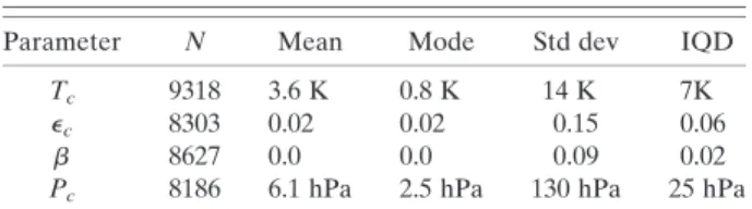
TABLE3. Statistics of the MODIS–CALIPSO comparisons for all ice clouds.
Parameter N Mean Mode Std dev IQD
Tc 9318 3.6 K 0.8 K 14 K 7K
ec 8303 0.02 0.02 0.15 0.06
b 8627 0.0 0.0 0.09 0.02
Pc 8186 6.1 hPa 2.5 hPa 130 hPa 25 hPa
TABLE4. Statistics of the AVHRR–MODIS comparisons for all ice clouds.
Parameter N Mean Mode Std dev IQD
Tc 9437 23.2 K 22.4 K 8.2 K 7.2 K
ec 8856 20.06 20.06 0.15 0.06
b 9051 20.01 0.0 0.09 0.02
of this weakness on the derived high-cloud amounts is explored. Figure 11 shows a comparison of the zonally averaged high-cloud amounts derived from August 2006 forNOAA-18/AVHRR,Aqua/MODIS, and CALIPSO.
Only data from the 0.58cells that have simultaneous data are included. These are the same data as used previously except that the requirement of a minimum amount of high cloud observed by CALIPSO is absent. Because FIG. 9. As in Fig. 8 but for the comparison ofec.
CALIPSO is the most sensitive of the instruments to the presence of optically thin high cloud, the CALIPSO results in Fig. 11 are shown as a function of the mini-mum allowedecvalue, denoted asec,min. For example,
the CALIPSO curve forec50.4 is derived from all cells
whereec#0.4 is ignored. The curves forec50.0
cor-respond to no filtering. The CALIPSO results are shown for ec,min 5 0.0, 0.2, 0.4, 0.6, and 0.8. The CALIPSO
high-cloud amounts decrease with increasing values of ec,min.
The results in Fig. 11 show that the unfiltered CALIPSO zonal high-cloud amounts are always larger than those from MODIS or AVHRR. In the tropics, MODIS and AVHRR tend to follow the CALIPSO result forec,min5
0.2. In the northern midlatitudes, MODIS and AVHRR follow theec,min50.4 curves. However, MODIS
high-cloud amounts tend to be larger by roughly 5% in the northern midlatitudes. Near the South Pole, AVHRR and MODIS disagree greatly, with the AVHRR zonal pattern more closely following the CALIPSO ec,min5
0.4 curve. It is important to note that the South Pole in August represents a difficult region for the AVHRR. Near the North Pole, the MODIS values follow the ec,min50.4 CALIPSO curve while the AVHRR values
actually exceed the CALIPSO values for zones pole-ward of 708N. In terms of high-cloud sensitivity, rep-resented by the corresponding value of ec,min, the
AVHRR and MODIS are more sensitive in the tropics than in the midlatitudes. In summary, these results in-dicate that the AVHRR, even with its flaws, does a good job in capturing the zonal distribution of high cloud relative to MODIS and CALIPSO. These results give confidence to attempts to extend cloud climate varia-bility research done with MODIS back to the 1980s and 1990s with the AVHRR.
10. Conclusions and future work
The goal of this paper is to explore the utility of a new split-window approach for the generation of a multi-decadal climatology based on AVHRR data of the cloud temperature, emissivity, and a microphysical pa-rameter. To be relevant, the split-window results must provide information beyond that provided by the other
methods applied to imager data to derive long-term cloud climatologies (VIS/IR and IR). The analysis shown here clearly demonstrates that the application of the split-window approach to the AVHRR data could form the basis for a new cloud climatology that could span from 1981 to the present, adding much to the in-formation currently available over this time period. A comparison of the split-window results relative to those from CALIPSO and Aqua/MODIS demonstrates and quantifies the strengths and weaknesses of the approach in a manner never possible before.
Based on the analysis presented here, the split-window method was shown to estimate accurately the values of ecandbfor high clouds with emissivities less than 1 (i.e.,
cirrus). For opaque ice clouds, the valuesTcagreed well
with those from MODIS and CALIPSO as expected. For semitransparent cirrus, the estimation ofTcwas shown
to be highly sensitive to the first guess. The accuracy of
Tcfrom the split-window method determined by
com-parison to CALIPSO was shown to be comparable than that from MODIS. The above weakness in estimating
Tc does not prevent the AVHRR from producing
global high-cloud distributions that agree favorably with both MODIS and CALIPSO. Because the split-window method applied to the AVHRR can perform these trievals during the day and night consistently, the re-sulting climatology of these parameters should add to the information currently available from existing satel-lite climatologies.
Another conclusion from this paper is that the MYD06 estimates of Tc and ec also perform well relative
to CALIPSO retrievals of Tc and to the CALIPSO/
AVHRR-based estimates ofec. MYD06 currently does
not derive any microphysical information from its infra-red channels. As done here, a simple computation of the cloud emissivity at 12mm would allow for an inclusion of bvalues within MYD06. Estimation of the cloud emis-sivities at other MODIS wavelengths such as 8.5 mm would allow for a more refined estimate of cloud mi-crophysics. Optimal use of 8.5, 11, and 12mm for cloud microphysics studies, such as provided by the Visible and Infrared Imager Radiometer Suite (VIIRS), continues to be a goal of this research.
Several steps remain before the goal of a 30-yr clima-tology from the split-window approach is completely realized. First, the split-window method described here will need to be applied to the entire AVHRR/2 and AVHRR/3 data record through the PATMOS-x project. This will result in a new climatology ofTc,ec, andband
layered cloud amounts that, as described above, should complement the existing information. In addition, the uncertainty estimates from the optimal approach will be used to place error bars on the long-term time series FIG. 11. Comparison of zonal distribution of high-cloud amount
fromNOAA-18/AVHRR,Aqua/MODIS, and CALIPSO/CALIOP for August 2006 for all coincident and collocated data. The dashed lines represent the CALIPSO values using different minimumec thresholds. Grid cells with CALIPSOecvalues below this are con-sidered clear.
derived from PATMOS-x. In the future, the resulting PATMOS-x time series will be analyzed to explore the variability in cirrus properties over the last three decades. Last, methods to ensure physical consistency of the cirrus cloud time series between the AVHRR record and that of its successor, VIIRS, will be explored.
Acknowledgments. The MODIS products were pro-vided by the NASA Level 1 and Atmosphere Archive and Distribution System (LAADS). The clear-sky ra-diative transfer model used here was provide by Mr. Hal Woolf of UW/SSEC; Dr. Bryan Baum and Mr. Amato Evan provided very significant reviews of this manu-script. The views, opinions, and findings contained in this report are those of the author(s) and should not be construed as an official National Oceanic and Atmo-spheric Administration or U.S. government position, policy, or decision.
APPENDIX
Infrared Forward Model and Derivation of the Kernel Matrix
The forward model for infrared radiances used here is the following:
I5 ecIac1TacecB(Tc)1Iclr(1 ec), (A1)
where I is the top-of-atmosphere radiance, Iac is the
radiance contribution from the region above the cloud, andIclris the clear-sky radiance. HereTacrepresents the
above-cloud transmission and the B operator is the Planck function. The cloud is represented by its cloud-top temperatureTcand its emissivityec.
The clear-sky transmission profiles are computed us-ing the Pressure Layer Fast Algorithm for Atmospheric Transmittances (PFAAST) radiative transfer model Li et al. (1998). The atmospheric profiles are provided by NCEP reanalysis data (Kalnay et al. 1996). The surface emissivity is provided by the surface emissivity database of Seemann et al. (2008).
Using the forward model given in Eq. (A1), the terms that compose the kernel matrix shown in Eq. (2) can be analytically derived. One term that is needed is the derivative of the 12-mm cloud emissivity with respect to the 11-mm emissivity given by
›ec,12
›ec,11
5b(1 ec,11)b 1. (A2)
For notational convenience, the termathat is repeated in several equations is defined as
a5Iac1TacB(Tc) Iclr. (A3)
Using the definitions of Eqs. (A1), (A2), and (A3), the elements of Eq. (2) are determined to be as follows:
›T11 ›Tc 5Tac, 11ec ›B11 ›Tc ›B11 ›T11 1 , (A4) ›T11 ›ec 5(a11) ›B11 ›T11 1 , (A5) ›T11 ›b 50, (A6) ›(T11 T12) ›Tc 5 ›T11 ›Tc Tacec,12 ›B12 Tc ›B12 T12 1 , (A7) ›(T11 T12) ›ec 5›T11 ›ec,11 (a12) ›ec,12 ›ec,11 , and (A8) ›(T11 T12) ›b 5(a12) ›B12 ›T12 1 ln(1 ec,11)(1 ec,12). (A9) REFERENCES
Baum, B. A., A. J. Heymsfield, P. Yang, and S. T. Bedka, 2005: Bulk scattering properties for the remote sensing of ice clouds. Part I: Microphysical data and models.J. Appl. Meteor.,44,
1885–1895.
Cooper, S. J., T. S. L’Ecuyer, and G. L. Stephens, 2003: The impact of explicit cloud boundary information on ice cloud micro-physical property retrievals from infrared radiances.J. Geophys. Res.,108,4107, doi:10.1029/2002JD002611.
Duda, D. P., and J. D. Spinhirne, 1996: Split-window retrieval of particle size and optical depth in contrails located above horizontally inhomogeneous ice clouds.Geophys. Res. Lett., 23,3711–3714.
Eleftheratos, K., C. S. Zerefos, P. Zanis, D. S. Balis, G. Tselioudis, K. Gierens, and R. Sausen, 2007: A study on natural and manmade global interannual fluctuations of cirrus cloud cover for the period 1984–2004.Atmos. Chem. Phys.,7,2631–2642. Giraud, V., J. C. Buriez, Y. Fouquart, F. Parol, and G. Seze, 1997: Large-scale analysis of cirrus clouds from AVHRR data: Assessment of both a microphysical index and the cloud-top temperature.J. Appl. Meteor.,36,664–675.
Heidinger, A. K., 2003: Rapid daytime estimation of cloud prop-erties over a large area from radiance distributions.J. Atmos. Oceanic Technol.,20,1237–1250.
——, and G. L. Stephens, 2000: Molecular line absorption in a scattering atmosphere. Part II: Application to remote sensing in the O2A band.J. Atmos. Sci.,57,1615–1634.
Inoue, T., 1985: On the temperature and effective emissivity de-termination of semi-transparent cirrus clouds by bispectral measurements in the 10 micron window region.J. Meteor. Soc. Japan,63,88–99.
Jacobowitz, H., L. L. Stowe, G. Ohring, A. Heidinger, K. Knapp, and N. R. Nalli, 2003: The Advanced Very High Resolution
Radiometer Pathfinder Atmosphere (PATMOS) climate da-taset: A resource for climate research.Bull. Amer. Meteor. Soc.,84,785–793.
Kalnay, E., and Coauthors, 1996: The NCEP/NCAR 40-Year Reanalysis Project.Bull. Amer. Meteor. Soc.,77,437–471. Li, J., W. Wolf, W. P. Menzel, P. F. van Delst, H. M. Woolf,
T. H. Achtor, and A. H. Huang, 1998: International ATOVS processing package: Algorithm design and its preliminary performance.Optical Remote Sensing of the Atmosphere and Clouds,J. Wang et al., Eds., (SPIE Proceedings, Vol. 3501), 196–206.
Marks, C. J., and C. D. Rodgers, 1993: A retrieval method for atmospheric composition from limb emission measurements.
J. Geophys. Res.,98,14 939–14 953.
Menzel, W. P., and Coauthors, 2008: MODIS global cloud-top pressure and amount estimation: Algorithm description and results.J. Appl. Meteor. Climatol.,47,1175–1198.
Miller, S. D., G. L. Stephens, C. K. Drummond, A. K. Heidinger, and P. T. Partain, 2000: A multisensor diagnostic satellite cloud property retrieval scheme.J. Geophys. Res.,105,19 955–19 972. Nieman, S. J., J. Schmetz, and W. P. Menzel, 1993: A comparison of several techniques to assign heights to cloud tracers.
J. Appl. Meteor.,32,1559–1568.
Parol, F., J. C. Buriez, G. Brogniez, and Y. Fouquart, 1991: In-formation content of AVHRR channels 4 and 5 with respect to the effective radius of cirrus cloud particles.J. Appl. Meteor., 30,973–984.
Pavolonis, M. J., A. K. Heidinger, and T. Uttal, 2005: Daytime global cloud typing from AVHRR and VIIRS: Algorithm description, validation, and comparisons.J. Appl. Meteor.,44,804–826. Platnick, S., M. D. King, S. A. Ackerman, W. P. Menzel, B. A. Baum,
J. C. Riedi, and R. A. Frey, 2003: The MODIS cloud products:
Algorithms and examples fromTerra. IEEE Trans. Geosci. Remote Sens.,41,459–473.
Rodgers, C. D., 1976: Retrieval of atmospheric temperature and composition from remote measurements of thermal radiation.
Rev. Geophys.,14,609–624.
Rossow, W. B., and R. A. Schiffer, 1999: Advances in under-standing clouds from ISCCP.Bull. Amer. Meteor. Soc.,80,
2261–2288.
Schwalb, A., 1982: The TIROS-N/NOAA A-G satellite series. NOAA Tech. Memo. NESS 95, 75 pp.
Seemann, S. W., E. E. Borbas, R. O. Knuteson, G. R. Stephenson, and H.-L. Huang, 2008: Development of a global infrared land surface emissivity database for application to clear-sky sounding retrievals from multispectral satellite radiance measurements.J. Appl. Meteor. Climatol.,47,108–123. Stowe, L. L., H. Jacobowitz, G. Ohring, K. R. Knapp, and N. R. Nalli,
2002: The Advanced Very High Resolution Radiometer (AVHRR) Pathfinder Atmosphere (PATMOS) climate dataset: Initial analyses and evaluations.J. Climate,15,1243–1260. Travis, D. J., A. M. Carleton, and S. A. Changnon, 1997: An
em-pirical model to predict widespread occurrences of contrails.
J. Appl. Meteor.,36,1211–1220.
Vaughan, M. A., S. A. Young, D. M. Winker, K. A. Powell, A. H. Omar, Z. Liu, Y. Hu, and C. A. Hostetler, 2004: Fully automated analysis of space-based lidar data: An overview of the CALIPSO retrieval algorithms and data products.Laser Radar Techniques for Atmospheric Sensing,U. N. Singh, Ed., (SPIE Proceedings, Vol. 5575), 16–30.
Zhang, M. H., and Coauthors, 2005: Comparing clouds and their seasonal variations in 10 atmospheric general circulation models with satellite measurements. J. Geophys. Res., 110,