Design and application of a wireless torque sensor for CNC milling

University of New Hampshire

University of New Hampshire Scholars' Repository

Master's Theses and Capstones Student Scholarship

Spring 2009

Design and application of a wireless torque sensor

for CNC milling

Jeffrey Scott Nichols

University of New Hampshire, Durham

Follow this and additional works at:https://scholars.unh.edu/thesis

This Thesis is brought to you for free and open access by the Student Scholarship at University of New Hampshire Scholars' Repository. It has been Recommended Citation

Nichols, Jeffrey Scott, "Design and application of a wireless torque sensor for CNC milling" (2009).Master's Theses and Capstones. 452.

DESIGN AND APPLICATION OF A WIRELESS TORQUE SENSOR FOR CNC MILLING

BY

JEFFREY SCOTT NICHOLS B.S., University of New Hampshire, 2007

THESIS

Submitted to the University of New Hampshire in Partial Fulfillment of

the Requirements for the Degree of

Master of Science in

UMI Number: 1466944

INFORMATION TO USERS

The quality of this reproduction is dependent upon the quality of the copy submitted. Broken or indistinct print, colored or poor quality illustrations and photographs, print bleed-through, substandard margins, and improper alignment can adversely affect reproduction.

In the unlikely event that the author did not send a complete manuscript and there are missing pages, these will be noted. Also, if unauthorized copyright material had to be removed, a note will indicate the deletion.

UMI

All rights reserved. This microform edition is protected against unauthorized copying under Title 17, United States Code.

ProQuest LLC

This thesis has been examined and approved.

Thesis Director, Dr. Robert B. Jerard Professor of Mechanical Engineering

Thesis Co-Direst©?;' Dr. Michael J. Carter Associate Professor of Electrical and Computer Engineering

SL,

Dr. Barry K. Fussell

Professor of Mechanical Engineering

Dr. L. Gordon Kraft

Professor of Electrical and Computer Engineering

Dr. Kent A. Chamberlin

Professor of Electrical and Computer Engineering

DEDICATION

ACKNOWLEDGMENTS

I would first like to thank Dr. Jerard for his enormous investment of time during the writing process of this thesis. His guidance and feedback was invaluable. Thanks to both Dr. Jerard and Dr. Fussell for their direction and insight during the course of my research. Thanks to Dr. Carter for his encouragement and help during my transition into graduate school. Thanks to Dr. Kraft and Dr. Chamberlin for finding time to be on my committee and review my thesis on short notice.

The support of the National Science Foundation under grant DMI-0620996 is gratefully acknowledged.

Special thanks goes to Chris Suprock, who developed the initial Smart Tool Holder. I am glad to have been able to contribute to the project.

I would like to thank my lab partners Brian, Chris, Corey, Cuneyt, Firat, Min, Raed, and Yanjun for their many insights and for providing a great working environment at the Design and Manufacturing Laboratory. I would also like to thank Adam Perkins, Kathy Reynolds, Tracey Harvey, and Sheldon Parent for the help they provided

throughout my graduate studies.

Finally, I would like to thank my family. Without their love and support I would not be the person I am today.

TABLE OF CONTENTS

Dedication iii Acknowledgments iv

List of Figures viii List of Tables xi Abstract xii Chapter 1: Introduction 1

1.1 Introduction 1 1.2 Thesis Overview 3 Chapter 2: Wireless Sensors 4

2.1 Introduction 4 2.2 Design Requirements 5

2.3 Design Description 9 2.3.1 Overview of the Smart Tool Holder Physical Design 9

2.3.2 Main Electronics Board Overview 11

2.3.3 Torque Measurement 13 2.3.4 Torque Drift Compensation 16 2.3.5 Temperature Measurement 17

2.3.6 Radio Transmitter 18

2.3.8 Indicator LEDs 19

2.3.9 Power 20 2.3.10 Battery Charging 24

2.3.11 Component Cost 25 2.4 Characterization and Calibration 25

2.4.1 Sampling Rate and Aliasing 25 2.4.2 Torque Calibration and Noise Level 27

2.4.3 Transmitter Latency 30 2.4.4 Battery Discharge Characteristics 31

2.4.5 Battery Charge Time 32

2.5 Summary 33 Chapter 3: Information Technology 34

3.1 Introduction 34 3.2 XML Schema 36 3.3 MATLAB Toolbox 39

3.4 Summary 42 Chapter 4: Applications of the Smart Tool Holder 43

4.1 Introduction 43 4.2 Force and Torque Model for a Chatter Simulator 46

4.2.1 Force Model 48 4.2.2 Torque Model 54 4.3 Chatter Simulator 55

4.4 Power Sensor 60 4.5 Summary 62 Chapter 5: Conclusions and Future Work 64

5.1 Conclusions 64 5.2 Future Work 65

5.2.1 Increase the Anti-Aliasing Filter Order 65 5.2.2 Replace Bluetooth Radio With Another Technology 65

5.2.3 Process Data On-Board 67 5.2.4 Add a Charging Temperature Sensor 67

5.2.5 Reduce Strain Gauge Temperature Sensitivity 68 5.2.6 Information Sharing Between Research Groups 69

5.2.7 eXist XML Database 69 5.2.8 Real-Time Controller for Chatter Suppression 71

5.2.9 Extension of Chatter Simulator 71

List of References 73 Appendix A: Smart Tool Holder Main Board Layout, Schematic and Parts 76

Appendix B: Charging Board Layout, Schematic and Parts 81

Appendix C: Additional Electronics Parts 85

Appendix D: XML Schema 86 Appendix E: Example XML Data File 89

Appendix F: Description of MATLAB Toolbox 92 Appendix G: Force and Torque Model Matrix Generation Program 97

LIST OF FIGURES

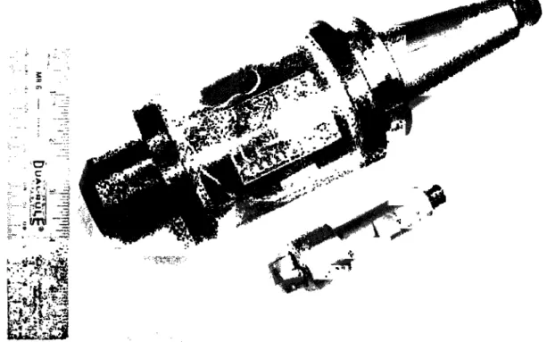
Figure 2.1: Smart Tool Holder (top) and sensor integrated cutting tool (bottom) 9

Figure 2.2: Smart Tool Holder physical layout 10 Figure 2.3: Smart Tool Holder physical connection diagram 10

Figure 2.4: Smart Tool Holder main electronics board 12 Figure 2.5: Smart Tool Holder main electronics board block diagram 12

Figure 2.6: Strain gauge bridge balancing circuit 16 Figure 2.7: Battery voltage monitoring circuit 24

Figure 2.8: Torque calibration curve 28 Figure 2.9: Ambient noise and histogram 28 Figure 2.10: Noise power spectral density 29 Figure 2.11: Round-trip latency of 1000 samples 30 Figure 2.12: Battery discharge curve with typical load 32 Figure 3.1: XML Schema for experiment results file 36

Figure 3.2: Example usage of the Fourier Analysis Tool 39 Figure 3.3: Example usage of the Average Plotting Tool 40 Figure 3.4: Example usage of the Ktc, Kte Regression Tool 42 Figure 4.1: Block diagram of chattering milling system 44 Figure 4.2: Example stability lobe diagram [Suprock, et al. 2008] 45

Figure 4.4: Angular limits of cutting 49 Figure 4.5: Chip thickness due to dynamic displacement 50

Figure 4.6: Tool runout magnitude and locating angle 51 Figure 4.7: Differential forces on a slice of a cutting tool 52

Figure 4.8: Simulink diagram for a mill 55 Figure 4.9: Simulink diagram for cutting forces from displacement 56

Figure 4.10: Simulink digram for displacement from cutting forces 56

Figure 4.11: Basic usage for chatter simulator 57 Figure 4.12: X and Y forces for a simulated cut at 4000 RPM (chatter) 58

Figure 4.13: X and Y forces for a simulated cut at 4300 RPM (stable) 58 Figure 4.14: X and Y forces for a simulated downmill using a 4-tooth cutter 59

Figure 4.15: Power sensor data (filtered for clarity) 61 Figure 4.16: Smart Tool Holder data (filtered to show average torque) 62

Figure A. 1: Top copper 76 Figure A.2: Bottom copper 76 Figure A.3: Top solder mask 77 Figure A.4: Bottom solder mask 77 Figure A.5: Top silkscreen 77 Figure A.6: Bottom silkscreen 77 Figure A.7: Main board electrical schematic 78

Figure B.l: Top copper 81 Figure B.2: Bottom copper 81

Figure B.3: Top solder mask 82 Figure B.4: Bottom solder mask 82 Figure B.5: Top silkscreen 82 Figure B.6: Bottom silkscreen 82 Figure B.7: Charging board electrical schematic 83

Figure F.l: XML Measurement Toolbox accessed from the MATLAB Start menu 92

Figure F.2: Main GUI 93 Figure F.3: XML database selection dialog 93

Figure F.4: Load from files dialog 94 Figure F.5: Subset dialog box 95

LIST OF TABLES

Table 2.1: Power supply current requirements 22 Table 2.2: LDO efficiency and battery power consumption 23

Table 2.3: Battery charge times 33 Table A.l: Main electronics board components 79

Table B.l: Charging board components 84 Table C.l: Additional Smart Tool Holder parts 85

ABSTRACT

DESIGN AND APPLICATION OF A WIRELESS TORQUE SENSOR FOR CNC MILLING

by

Jeffrey Scott Nichols

University of New Hampshire, May, 2009

A Smart Machining System for Computer Numerical Control (CNC) Milling continually adjusts the cutting process parameters to optimize for cutting tool life and material removal rate. The system depends on sensors to gather information from the machine during cutting, but commercially available sensors detract from the effectiveness of the cutting system by lowering the system stiffness. This research focuses on the

development of the electronics for a Smart Tool Holder (STH) and potential applications such as measurement of mechanical cutting power and suppression of chatter. The STH is a standard milling tool holder modified to hold a torque strain gauge bridge, a

thermocouple and a Bluetooth radio transmitter. The STH is meant to overcome some of the different limitations imposed by bed dynamometers, microphones and spindle power sensors without reducing the system stiffness. Comparison of the mechanical power estimates from the STH and a conventional power sensor showed 10% difference.

CHAPTER 1

INTRODUCTION

1.1 Introduction

A Smart Machining System for CNC Milling [Xu 2007] utilizes sensors to gather information about the cutting process and responds by updating the feedrate and spindle speed of the cutting process to optimize various metrics, such as material removal rate (MRR), tool life or surface finish. Process updates can be made either off-line during the process planning stage or on-line during cutting.

A Smart Machining System is only as good as the information it gathers. There is a great need for sensors that can provide detailed information about the cutting process. It is desirable get this information without significantly altering the dynamics of the milling system. Historically, sensors used in machining have fallen into two categories: sensors that directly measure cutting forces and change the system dynamics, and sensors that don't alter dynamics and only indirectly provide information about the cutting forces.

An example of a sensor providing direct access to the cutting forces is a Kistler force dynamometer. It can provide cutting force signals with high accuracy, but it lowers the stiffness of the milling system. Lower stiffness adversely affects part tolerances and can cause chatter problems. Furthermore, the Kistler force dynamometer is an expensive

envelope. The high cost of the Kistler dynamometers (approximately $30,000) and their invasive nature make them unsuitable for widespread adoption by manufacturing companies.

An example of a sensor that does not change dynamics is a microphone. The auditory data from a microphone can be used to measure relative tool wear by comparing the signal levels from a sharp tool to that of a worn tool [Desfosses 2007]. Microphone data can also be used to predict regenerative chatter through the use of systems such as the Harmonizer [Delio 1992]. Microphones, however, are prone to noise from external sources, such as other machines on a shop floor. Furthermore, microphones cannot easily be used to estimate the forces, making them unsuitable for some applications such as feedrate optimization [Jerard, et al. 2006].

Spindle motor power sensors do not alter the dynamics of the machining system, and can be utilized to estimate the mechanical cutting power. The mechanical power is directly proportional to the average tangential cutting force. From the mechanical power it is possible to perform feedrate optimization and tool wear monitoring [Desfosses 2007, Cui 2008]. To obtain the mechanical power, the electrical power of the unloaded spindle, or tare power, must first be measured. Because the tare power can change with spindle speed and motor temperature, acquiring a good estimate of the tare power can be

difficult. Estimating the mechanical power also requires a motor efficiency curve, which is expensive and time-consuming to determine. Furthermore, the spindle power sensor has a time constant which is long relative to the the tooth passing interval [Xu 2007]. Because of their long time constants, spindle power sensors are not suitable for

measuring high-frequency phenomena such as chatter.

Acquiring good information about the cutting process is only part of the problem, however. A Smart Machining System also needs to be able to communicate with its environment by providing sensor and status information for viewing and archival. There has been some work to standardize the inputs and outputs of machining systems through the use of open and extensible file formats. MTConnect [MTConnect] has been aimed at standardizing the status output across different component manufacturers, and NCML [Ryou 2001, Ryou and Jerard 2001, Schuyler 2005, Jerard and Ryou 2006] has been aimed at creating a standardized representation of the part to be cut. There is still, however, a need for a standardized file format for data archival for machining systems.

This research had two distinct focuses: the development and application of a wireless torque sensor, and the development of a new file format for archiving machining sensor data. These focuses, while distinct, are united in their goal of improved

productivity for Smart Machining Systems and machine operators. 1.2 Thesis Overview

There are five chapters in this thesis. Chapter 1 provides background for the subject. Chapter 2 describes the requirements and development of a torque sensor for milling. Chapter 3 details a new file format designed to store cut configuration data alongside sensor data for the purposes of archival. Chapter 4 describes applications of the torque sensor. Chapter 5 gives a summary of the thesis and describes future work.

CHAPTER 2

WIRELESS SENSORS

2.1 Introduction

Sensors are an integral part of any information based machining framework. They are the eyes and ears of the system. Wireless sensors have the advantage of being capable of being deployed in locations where conventional sensors would be infeasible, such as on a rotating cutting tool. Sensors located on the cutting tool have more direct access to the cutting forces than to sensors located elsewhere in the machine, as the signal is not propagating through other material before being measured.

The cutting forces provide key information about the cutting process. They can be used to track wear, as the forces are lowest on a sharp tool, and increase over the lifetime of the cutting tool. Knowledge about the cutting forces can also be used during toolpath generation to optimize feedrates [Jerard, et al. 2006]. Furthermore, the cutting force frequency content can be analyzed to detect chatter modes as will be discussed in more detail in Chapter 4.

Wear monitoring and feedrate optimization have typically been performed using output from non-invasive spindle power sensors, but these power sensors do not have sufficient bandwidth to provide information about chatter conditions. Furthermore, it is necessary to know the spindle motor efficiency curve, requiring an expensive and time

consuming calibration. This efficiency curve can be difficult to determine outside of a research environment. Furthermore, the unloaded power of the motor, or tare power, changes with temperature, complicating the acquisition of accurate power measurements.

This chapter outlines the design requirements and development of the Smart Tool Holder, a milling tool holder with embedded torque and temperature sensors. Torque is directly proportional to the tangential cutting force. The Smart Tool Holder captures data from these sensors and transmits the signal wirelessly to a receiving computer where it can be recorded and analyzed. The purpose of the Smart Tool Holder is to provide the functionality of the power sensor for wear tracking and feedrate override, while also providing higher bandwidth information that can be used to analyze regenerative chatter.

Temperature plays a critical role in tool life [Drozda, et al. 1983]. Excessive heat accelerates tool wear. A temperature sensor embedded in the cutting tool may prove useful for applications in tool wear monitoring and tool wear research.

2.2 Design Requirements

The goal of the Smart Tool Holder is to capture high bandwidth torque data and low bandwidth temperature data during the milling process and send it wirelessly to a PC. The following list summarizes the design requirements for the Smart Tool Holder:

• The device must capture the DC component of torque • The torque signal's bandwidth must be at least 2500Hz.

• The sampling rate on the torque signal must be high enough to prevent aliasing. • Must have the RMS torque measurement noise below 0.15N-m.

• The wireless transmitter must be capable of transmitting data without distortion. • The wireless transmitter must be capable of sending data to a receiving PC at least

10 meters away in a machining environment.

• The device must have less than 100ms of latency between the acquisition of a torque sample and the reception of that sample on the PC.

• Provide a mechanism to bring the long-term drift in the torque signal to zero. • Run for at least 1 hour after charging the device.

• Charge in less than two hours after an hour of usage.

• The physical design of the electronics must fit within the space between two concentric cylinders of height 5.08cm and diameters 4.45cm and 5.71cm. • The cost of the electronics should be less than $150.

Each of these requirements is meant to ensure that the device is usable in a machining environment and useful for machining related research.

The DC component of torque is important for capturing the average mechanical power. The average power can be used to estimate the coefficients for the cutting model described in [Altintas 2000], which can be used as a cutting-condition independent indicator of tool wear [Desfosses 2007, Cui 2008]. The mechanical power is a simple function of the torque Tand the spindle speed:

P{t

)

T(t)u>=T(t)2ZJJP*-, (2.1)

where Tis given in N-m, and P is in W. Therefore, to calculate the average power, the average torque (or DC torque) is needed.

The 2500Hz requirement on bandwidth is meant to ensure that the device can capture the frequencies of interest with minimal distortion. Implicit in this requirement is that the passband be relatively flat. A bandwidth of 2500Hz allows the device to capture the tooth passing frequency and nineteen harmonics for a two tooth cutter rotating at 7,500 RPM.

The sampling rate of the torque acquisition system must be high enough to prevent high frequency components from aliasing into the signal's passband. The Nyquist-Shannon sampling theorem states that the sampling frequency must be at least twice the bandwidth of the signal, though in practice the sampling rate must be much higher.

The RMS level of the noise must be below 0.15N-m. This is to allow torques from a cut with low forces to be measured. The maximum measurable temperature must be larger than 900°C to ensure that the device can measure typical cutting temperature [Drozda, et al. 1983].

The requirement for no digital distortion is based on fact that the analysis algorithms have not yet been firmly established, and lossy compression may render certain types of analysis ineffective. Once the analysis algorithms are more firmly established and understood, some types of lossy compression may become acceptable.

The wireless transmitter must be capable of sending data over a distance of at least 10 meters in a machining environment. This is based on the expected use of the device. It will be used in noisy machining environments (e.g. spindle motor running, coolant running, and metallic chips being removed from the workpiece), so the

transmitter must be capable of handling the interference without degrading the performance. The 10 meter requirement is meant to ensure that the device can be effectively used with any placement of the receiving PC.

The latency requirement of less than 100ms between the sampling of torque and the reception of the sample on the PC is meant to provide a upper bound on the delay in the feedback path for the analysis of control strategies. This is primarily aimed toward chatter avoidance control strategies, since the detectable buildup of regenerative chatter is on the order of seconds. This is in contrast to tool breakage, which can be on the order of milliseconds. Tool wear, on the other extreme, happens over minutes or hours.

Since many torque sensor technologies drift over their lifetime, the device should contain a mechanism to compensate for this drift, either in software or in hardware. Without compensation, the DC component of torque would only be valid directly after a calibration, and power estimation would be prone to error.

The hour run time requirement is there to allow the device to perform over the course of a typical cutting run. Implicit in this requirement is that the performance of the device be consistent over the hour of running. A shorter run time would limit the general usefulness of the device.

Similarly, the charge time requirement is meant to limit the downtime of the tool. With too long a charging period, the tool could not be used often enough to make it a useful product.

The constraint on the physical dimension of the electronics is imposed by the rest of the design for the Smart Tool Holder. The stock tool holder has a diameter of 4.45cm,

and the protective shroud has an inner diameter of 5.71cm, and the electronics must fit within the space between these. The height of 5.08cm is imposed by the height of the base tool holder and the location of its set screw.

The cost of the components must be less than $150 to ensure that the finished product is economical to produce.

Figure 2.1: Smart Tool Holder (top) and sensor integrated cutting tool (bottom)

2.3 Design Description 2.3.1 Overview of the Smart Tool Holder Physical Design

The physical realization of the Smart Tool Holder is shown in Figure 2.1. The device consists of a tool holder and a removable cutting tool. The tool holder was created from a commercially available Parlec Weldon Shank C40 tool holder with a 6" (15.24cm) overhang, modified to house the main electronics (detailed in Appendix A), battery and

is a Sandvik 390 insert holder that has been modified to hold the torque and temperature sensors. The locations of the major components are indicated in Figure 2.2 and the connections between them are shown in block diagram form in Figure 2.3.

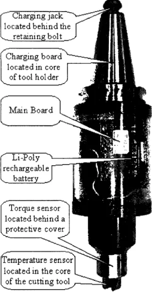
Charging jack located behind the , retaining bolt Charging board located in core of tool holder Main Board ' Li-Poly ^ rechargeable y. battery _ Torque sensor located behind a protective cover f f e n s u r e sensor

located in the core of the cutting tool

Figure 2.2: Smart Tool Holder physical layout

r~

V

physical connection diagram

The charging jack is located behind the spindle retaining bolt to protect it from the fluid and metal chips present during cutting operations. The charging board handles all of the battery monitoring and voltage regulation tasks necessary during the charging of the

Lithium-Polymer battery. The main electronics and battery are both housed within a transparent Lexan shroud around the tool holder body to allow viewing of the indicator lights while still providing sufficient protection to the components during the metal cutting process.

The torque strain gauge bridge is mounted on the shank of the removable cutting tool and covered by a protective aluminum shield. This shield prevents the strain gauges from being damaged by sharp chips being produced at the cutting interface. The

thermocouple for measuring the temperature is located along the central axis of the removable cutting tool, equidistant between the two cutting inserts. A connector on the back of the tool mates with a connector in the core of the tool holder and provides an electrical connection between the sensors and the main electronics.

2.3.2 Main Electronics Board Overview

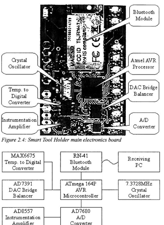
The complete layout, electrical schematic and parts list for the main electronics board is contained in Appendix A. The main electronics board (see Figure 2.4) holds the processor, radio transmitter and circuitry necessary for amplifying and digitizing the sensor signals. The crystal oscillator helps the processor maintain the accurate timing necessary for communicating with the radio module. The torque signal is passed through an instrumentation amplifier to increase the signal magnitude and then it is put into an analog to digital converter (A/D converter). A digital to analog converter (DAC) adds or removes current from one side of the torque strain gauge bridge to bring the output to zero. The thermocouple signal is put into a MAX6675 chip, a specialized temperature to digital converter that performs all the necessary steps to convert the non-linear

thermocouple output into an accurate temperature measurement. An interconnect diagram for these electrical systems on the main board is shown in Figure 2.5. The dimensions of the board are 3.048cm in width and 4.826cm in height. These dimensions ensure that it can fit between the tool holder body and the Lexan shroud.

Crystal Oscillator Temp, to Digital Converter Instrumentation Amplifier Bluetooth Module Ataiel AVR Processor DAC Bridge Balancer A/D Converter

Figure 2.4: Smart Tool Holder main electronics board

MAX6675 Temp, to Digital Converter AD7391 DAC Bridge Balancer AD8557 Instrumentation Amplifier RN-41 Bluetooth Module ATmega 164P AVR Microcontroller AD7680 Conv erter Receiving PC 7.3728MHz Crystal Oscillator

2.3.3 Torque Measurement

Strain gauges configured in a Wheatstone bridge can measure the torsional strain on a shaft, while rejecting the strain from bending and compression. The bridge also helps to reduce the effects of thermal strain. The torsional strain, T , that the bridge measures on the removable cutting tool is given by:

TD

T=2JG> <2'2>

where Tis the torque in N-m, Dis the diameter in meters, J is the polar moment of inertia in m4, and G is the shear modulus of the material in Pascals. The polar moment of inertia, J, of the cutting tool can be approximated by the moment of inertia for a solid cylinder:

J=f2D\ (2.3)

Using a diameter of 1.905cm and a typical shear modulus for steel of 80GPa, the relationship between torsional strain and torque on the removable cutting tool becomes:

v 3.885* 10~6 nA.

r=T . (2.4)

N-m

The change in voltage, A V, across the strain gauge bridge is a function of the gauge factor of the strain gauges, ks, the torsional strain, T , and the applied voltage, V:

AV=ksrV. (2.5)

Using an applied voltage of 3.1V (the rationale behind this voltage is discussed in Section 2.3.9), the ratio between torque and output voltage is:

AV , 12.04* 10~6V „„

This relationship is only an estimate, since the exact shear modulus of the material was not measured. The equation does, however, convey order of magnitude information about the relationship.

Wire strain gauges were chosen because they have a gauge factor of ks=2, which is

sufficient to get the minimum torque of 0.15 N-m into the microvolt range. This gives a theoretical voltage to torque ratio of 24.08* l(T6*V/N-m . Semiconductor strain gauges provide a much higher gauge factor, but at a higher cost. Semiconductor gauge factors are typically anywhere from 100 to 150.

Because the output voltage of the bridge is small, an instrumentation amplifier is needed to amplify the signal into a voltage range usable by the A/D converter. The instrumentation amplifier also converts the differential signal into a single ended signal for use with a standard A/D converter. The Analog Devices AD8557 instrumentation amplifier was selected because it was one of only a few devices that provided

programmable gain. The programmable gain allows the microcontroller to reduce the scale of the torque signal during heavy cuts, preventing the A/D converter from saturating and clipping the waveforms. The alternative is to select an instrumentation amplifier with a fixed gain low enough to encompass the heaviest cutting conditions, but the drawback is decreased sensitivity to lighter cutting conditions. The AD8557 has a minimum gain of 28, and a maximum gain of 1300. The gain of 1300 is the default gain in this design.

The A/D converter selected was the Analog Devices AD7680 as it contained a Serial Peripheral Interface (SPI), had 16-bit resolution, and provided sufficient sampling rate in a small package with a low cost. The SPI port allows simple interfacing with a

microcontroller. Many other A/D converters would have provided similar functionality. A first order RC low-pass filter between the instrumentation amplifier and the A/ D converter acts as an anti-aliasing filter. A 5.6kohm resistor and lOnF capacitor provide a corner frequency of approximately 2.84kHz. This provides more than the required 2.5kHz bandwidth. The sampling frequency of the A/D converter is set at 10.24kHz. The testing for aliasing is described in Section 2.4.1.

The gain of 1300 in conjunction with a 16-bit A/D means that the resolvable voltage on the bridge is:

AV= 3'1 V, =39.39nV (2 7)

1300*216 " { }

The resolvable torque is (assuming a shear modulus of 80GPa):

T= —^ =0.003021 N-m (2 8)

12.04*10~6V/N-m ' v ' '

This resolution, however, is only possible in a system without noise (or in a system with almost no bandwidth). Since the strain gauges are resistive, they are subject to Johnson-Nyquist noise, or thermal noise. The RMS voltage for this noise is given by:

Vnois=J4kBTRAf, (2.9)

where kB is Boltzmann's constant, T is the Kelvin temperature, R is the resistance of the

bridge, and A f is the width of the frequency range being sampled. A first order filter, such as the one employed as an anti-aliasing filter, has a noise equivalent bandwidth of

1.5 times the corner frequency. For the 350 ohm strain gauge bridge at room temperature, the thermal noise is:

F6n£/ge=V4-1.38066*10"23J/K-300K-350O*1.5*2.84kHz=157.17nV. (2.10) Another source of noise is the instrumentation amplifier. The AD8557 is rated at an input noise level of 32nV/VHz. The voltage noise from this is:

Vam_amp =32nV/VHz*Vl.5*2.84kHz=2.089uV (2.11)

This is a significantly larger source of noise than the strain gauges. The combined noise from these sources is:

F„o,,,= V(l57.17nV)2+(2.089uV)2=2.095 uV The torque corresponding to the voltage noise is:

7 , = 2.095uV/ 24.08uV/N-m = 0.0870N-m

(2.12)

(2.13) This means that the minimum torque of 0.15 N-m is, at least in theory, feasible. The testing to verify this result is described in Section 2.4.2.

2.3.4 Torque Drift Compensation

+ 3- l u

4

DAC

~5

End

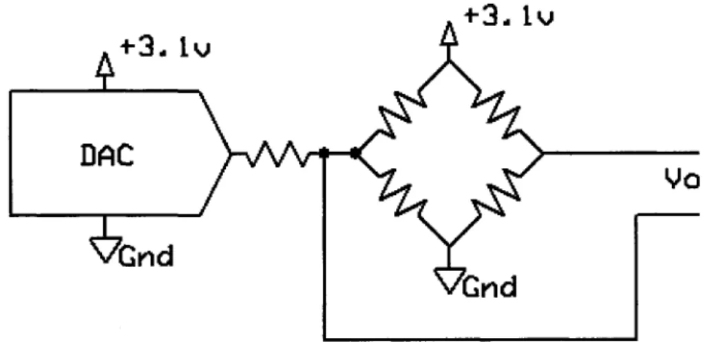
Figure 2.6: Strain gauge bridge balancing circuit

Manufacturing variation of the individual strain gauges and drift over the product lifetime can cause the output of a Wheatstone bridge to have a measurable offset at zero

torque. To compensate for this, a DAC was added to apply voltage through a resistor to one side of the bridge in order to bring the differential output signal to zero (see Figure 2.6). This process of balancing the bridge is performed whenever the Smart Tool Holder is powered on (this adds an additional requirement that there be no applied torque when the device is activated).

The DAC selected was a AD7390. It was selected because it provided an SPI interface (again, for ease of connecting to the microprocessor), had sufficient accuracy for balancing the strain gauge bridge, and had a low cost. Again, the specific choice of the DAC was more or less arbitrary, and many other converters would have provided similar functionality.

2.3.5 Temperature Measurement

Thermocouples were chosen for the temperature sensing technology because of their wide temperature range. Type-K thermocouples were selected because of their availability and the existence of commercial compensation chips. The MAX6675 was selected for the cold junction compensation chip because it handles the digitization directly. Cold junction compensation removes the dependence on the ambient

temperature from the measurement of the thermocouple. This allows simple and easy integration with the microcontroller.

Resistive temperature devices (RTDs) were rejected as a possibility because their low tolerance for vibration and because of their smaller input range. The alternative to the MAX6675 was to use an instrumentation amplifier and A/D to determine the voltage on the thermocouple and an additional temperature sensing IC to determine the cold junction

temperature. These two measurements could then be transformed into a temperature measurement. This possibility was rejected because of the additional complexity and board space usage, though it does have the potential to offer more accuracy than the MAX6675.

2.3.6 Radio Transmitter

The Roving Networks RN-41 Bluetooth Module was selected for the role of transmitting data to a PC. The use of Bluetooth [Bluetooth] allows any PC with Bluetooth support to utilize the device. Additionally, for computers without native Bluetooth

support, there are commercially available dongles that add Bluetooth functionality to USB enabled PCs. The RN-41 uses the Bluetooth Serial Port Profile (SPP) and appears as a virtual COM port on the host computer, providing a simple interface for the software developer.

While the Bluetooth audio profiles could conceivably be used for sending the sensor data, they would introduce undesirable distortion as part of the compression, and may lose portions of the data due to interference. The SPP on the other hand does not alter the data, and provides a reliable connection (meaning data not received is retransmitted).

Many of the Bluetooth alternatives do not have sufficient transmission rates to stream 160kbps (16-bit samples at 10kHz) to a PC. Those that do have acceptable

transmission rates require extra design work to develop the receiving hardware for the PC side. For this reason, Bluetooth was selected for the radio protocol. The RN-41 was chosen over other Bluetooth modules because of its compact size and ease of use. The

RN-41 is advertised as supporting sustained data rates up to 240kbps, and a range of up to 100 meters.

Latency is not specified for the RN-41, so testing was required. This procedure is described in Section 2.4.3.

2.3.7 Processor

The Atmel AVR series of 8-bit microcontrollers was selected for the central processor. Specifically, the ATmegal64P was chosen because it offers the ability to have two separate SPI ports in addition to a universal asynchronous receiver transmitter (UART). The two SPI ports are necessary because the A/D converter's SPI connection transmits much more quickly than the DAC's and thermocouple converter's SPI connection can handle. Having separate SPI ports for the high and low speed

transmissions simplifies the design of the hardware and software. The UART is needed to communicate with the RN-41 Bluetooth Module. Because of the high degree of timing accuracy needed for reliable UART transmission, an external crystal oscillator was provided to the microcontroller. The oscillator frequency of 7.3728 MHz allows integer division to the UART baud rates supported by the RN-41.

Many other microcontrollers would be suited for the task of processing on the Smart Tool Holder, but the AVR series of microcontrollers was selected because an Atmel STK500 AVR hardware programmer was already available during the development phase of the electronics.

2.3.8 Indicator LEDs

the current status of the Smart Tool Holder to a user. These lights are each independently controllable by the microcontroller. There are three green lights, three yellow lights and two red lights in a vertical line along the right edge of the main electronics board.

The RN-41 Bluetooth module is connected to two indicator LEDs. The first, a blue LED, indicates the current device state by different intervals of blinking. It blinks slowly when the RN-41 is in discoverable mode, blinks quickly when in configuration mode, and is solid during an active connection. The second LED, a green one, only shows connection status. It turns on when the device has an established connection to a PC, and is off otherwise. Further details about these indicators can be found in the RN-41 manual.

There is also a red LED that indicates battery charging status. The charging circuitry turns the indicator on when the battery is being charged, and off otherwise. 2.3.9 Power

Because the Smart Tool Holder's electronics use a significant amount of power (see Table 2.1), only battery based power systems were considered. Solar panels and energy harvesting devices weren't capable of supplying the necessary power without introducing extra complications or prohibitive expenses. Lithium-Polymer was selected for the battery technology because of its high energy density, allowing small, light-weight batteries to power the device.

A 430mAh capacity battery was selected to power the electronics, which provides a working time of around 4 hours between charges under normal usage. Larger capacity batteries did not meet the space requirements imposed by the shroud. This battery has a maximum discharge rate of 6A and a maximum charge rate of 0.4A. The design only

calls for one battery, but with careful cable management, there is sufficient space within the shroud to add a second battery in parallel with the first. A second battery would effectively double the running time of the Smart Tool Holder, but would also double the charging time (without redesigning the charging circuitry to safely support charging two batteries at maximum current). Further discussion will be limited to Smart Tool Holders containing only a single battery.

Since the battery voltage varies with the remaining capacity, it is necessary to use a voltage regulator to provide a constant supply voltage. A single 3.1V low-dropout (LDO) regulator was chosen to power the strain gauge bridge, conditioning circuitry and the digital electronics. The LED indicator lights use the unregulated supply since

variations in output intensity are acceptable. Another alternative to the LDO regulator was a buck converter, a switching power supply designed to output a lower voltage than the input voltage. The buck converter has higher power efficiencies when the input voltage is significantly higher than the output voltage, but has similar efficiencies to a LDO for the case of a 3.7V Lithium-Polymer battery with 3.1V output voltage. Buck converters were rejected because their higher component cost, increased power supply noise, and larger physical footprint.

The acceptable regulated voltage was between 3.0V and 3.6V as determined by the minimum and maximum supply voltage rating of the various components. The lower the chosen supply voltage, the more battery power can be extracted before dropping below the acceptable level. For this reason, the 3.1V level was chosen, to allow variation in the regulator to stay within the component limits, while still taking advantage of most

of the battery capacity. Component RN-41 Bluetooth Module ATMegal64P Microcontroller

MAX6675 Temp, to Digital Converter AD7680 A/D converter

AD7390 DAC

AD8557 Instrumentation Amplifier 350 ohm Strain Gauge Bridge Total (Regulated)

LED Indicator Lights (Unregulated) Total (Unregulated)

Max. Current (mA) 100 9 1.5 2.8 0.1 1.8 8.9 124.1 100 224.1

Average Current (mA) 30 8 0.7 2.8 0.1 1.8 8.9 52.3 50 102.3

Table 2.1: Power supply current requirements

The maximum and average current usages for the various components are shown in Table 2.1. The average current listed for the RN-41 Bluetooth Module is the average during transmission. The current usage is around 25mA when not connected to a PC. From the table, the sum of the regulated maximum currents is 124.1mA, meaning that the regulator must be able to supply a peak demand of at least this much.

LDO regulators have power efficiencies of approximately V0UT/VIN, since the

current into the regulator, IiN, is nearly the same as the current out of the regulator, IOUT

(there is a small quiescent current, Iq, but it is generally much, much smaller than I0UT):

_* OUT _V OUT* * OUT _ * OUT** OUT _ 'OUT ,~ , . . PIN V IN* I IN V lN*\I OUT + Iq) Vm

So for a 3.1 V regulator running off a Lithium-Polymer battery with a maximum cell voltage of about 4.0V, the efficiency is 77.5%. Since the input voltage drops as the battery is depleted, the efficiency increases to a maximum of 96.9% just before the output

voltage starts to drop below its regulation level (assuming a regulator drop out of 1 OOmV, where VIN = lOOmV + 3.1V). The efficiencies and power consumptions are summarized in Table 2.2. Battery Voltage Full (4.0V) Typical (3.7V) Empty (3.2V) LDO Efficiency (%) 77.5 83.8 96.9 Max. Power (mW) 896 829 717 Average Power (mW) 409 379 327

Table 2.2: LDO efficiency and battery power consumption

Ideally, the 430mAh capacity battery will supply the average current of 102.3mA for 252 minutes. Similarly, the battery will supply the maximum current of 224.1mA for

115 minutes. In practice, however, the voltage from the battery will drop below the acceptable V[N of 3.2V before the battery is completely depleted. The exact amount of usable capacity depends on the discharge rate, battery age, and temperature, but is generally between 80% and 95%. Even so, the worst case scenario of continuous 224.1mA of current with only 52% of the capacity being usable still meets the design requirement of a 1 hour run time. The run-time testing results are shown in Section 2.4.4.

The Texas Instruments TPS73131 regulator was chosen for this design. It allows input voltages up to 5.5V and has a drop out of 100mV. It can supply a constant 150mA, above the necessary peak demand of 124.1mA. Many similar regulators exist, but the TPS73131 was chosen because of its low cost.

One additional design feature was to include two 1 OOkohm resistors in a voltage divider configuration across the battery, with the center terminal going to one of the processor's internal A/D converters (the internal A/D converters were not used for torque

this monitoring circuit (the schematic of the entire board is contained in Appendix A). Using this circuit, the processor can monitor a battery voltage up to 6.2V (voltages beyond this level violate the microcontroller's input voltage ratings).

3 . 7 V

•100k

.100 k

1

+ 3 .

ADC

'Grid

Figure 2. 7: Battery voltage monitoring circuit

2.3.10 Battery Charging

The complete layout, schematic and parts list for the charging board is contained in Appendix B. Because of the complexities involved with charging Lithium-Polymer batteries, a commercial battery charging chip was selected. The TI BQ2057 advanced linear charge management IC provides conditioning, constant current, and constant voltage charging. The BQ2057 was selected for its simple integration and low cost. Another charging solution, the Texas Instruments BQ24001 was another option with the advantage of not needing an external transistor, but it was eventually rejected because of its requirement of soldering a thermal pad to the PCB. This requirement could not be met by the production capabilities during prototyping.

The charging board with the BQ2057 was designed to limit the charging current to 350mA. This limit was to keep the charging current below the battery's 400mA limit. The exact charging time depends on how deeply the battery was depleted. The charge time

testing is described in Section 2.4.5. 2.3.11 Component Cost

The cost of the individual main electronics board components is listed in Appendix A. These parts total to approximately $82.92. The cost of the charging board components is listed in Appendix B. These parts total to approximately $4.72. The miscellaneous other electronic components necessary for the design are listed in Appendix C. These parts total to approximately $33.14. The sum of these component costs is $120.78. This does not include the printed circuit board fabrication cost, which is roughly $20 at low volumes per pair of main board and charging board. This brings the cost of materials to around $140, which is less than the target of $150.

2.4 Characterization and Calibration

While most of the design requirements were met by component choice, some needed to be tested to ensure compliance. The list of design requirements not guaranteed by component choice is:

• The sampling rate on the torque signal must be high enough to prevent aliasing. • Must have the RMS torque measurement noise below 0.15N-m.

• The device must have less than 100ms of latency between the acquisition of a torque sample and the reception of that sample on the PC.

• Run for at least 1 hour after charging the device. • Charge in less than two hours after an hour of usage. 2.4.1 Sampling Rate and Aliasing

magnitude of the transfer function for the filter is given as follows:

| g ( / ) l =

V i

( / / 2 . « 4 m z ) -

'

This means that at the corner frequency of 2.84kHz, the torque signal will be attenuated to 70.71% of its original value. The filter is designed to prevent high frequency

components from entering the A/D converter where they can alias into parts of the spectrum containing the torque information. The sampling frequency of the A/D

converter is 10.24kHz. The aliasing isn't an issue until the frequencies start aliasing back into the passband. This happens when the frequencies pass above 10.24kHz - 2.84kHz = 7.40kHz. At this frequency, the signal magnitude is 35.85% as calculated by equation (2.15). Frequencies at the sampling rate get aliased to DC, and their magnitude is 26.74%.

These attenuation levels are not sufficient to prevent noticeable aliasing. There are several solutions to this. The most obvious solution is to increase the order of the filter to provide more attenuation at the higher frequencies. The current hardware cannot,

however, be easily modified to support a higher filter order, so a redesign would be necessary. Another solution is to increase the sampling rate of the A/D converter. This gives a higher Nyquist frequency, giving the existing filter more opportunity to filter frequencies before they alias. A significantly higher sampling rate cannot be easily achieved by the current system for two reasons. The first reason is that the Bluetooth transmitter is limited to 260kpbs, meaning the maximum possible theoretical sampling rate is 16.25kHz, though in practice the limit is closer to 12kHz due to protocol overhead. The second limitation is that a large portion of the current system's processing power is

already consumed by handling the 10.24kHz sampling rate, and a higher rate may exceed the capabilities of the microcontroller. Another solution is to reduce the bandwidth of the device by lowering the anti-alias filter's corner frequency. To be effective, however, lowering the corner frequency would require the bandwidth to be reduced below the level of the design requirement of 2.5kHz.

The current configuration of the system does not sufficiently attenuate high frequency signals, but on the other hand, the mechanical systems which the Smart Tool Holder is designed to monitor do not typically generate high frequency signals. The high frequency components being measured are primarily noise. This means that the device will experience more noise than otherwise expected.

2.4.2 Torque Calibration and Noise Level

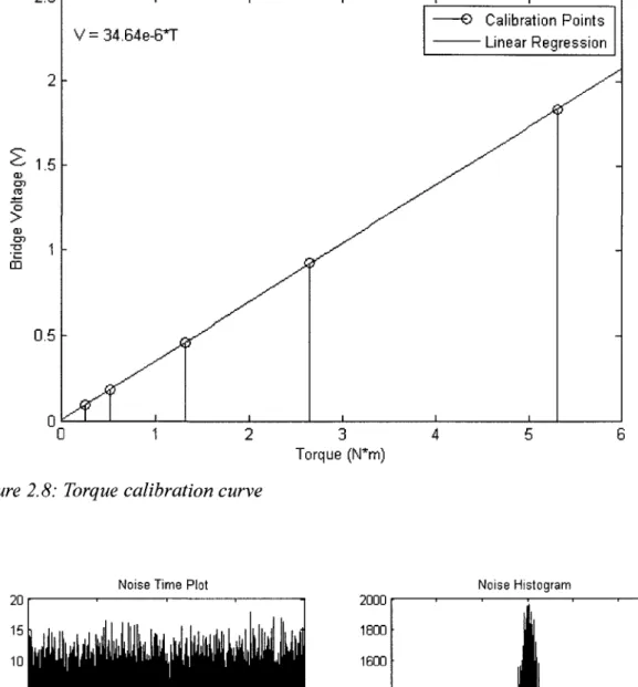
The torque was calibrated using weights hung from a moment arm. The tool holder was mounted horizontally in a vice. A long clamp was attached to the insert holder to provide a place to hang weights to generate a torque on the instrument. The setup was leveled, and five weights of varying sizes were hung one at a time from the clamp. The results of the calibration are shown in Figure 2.8. The length of the moment arm was 27.07cm. The weights had masses of lOOg, 200g, 500g, 1kg, and 2kg.

The voltage to torque ratio of 34.64* 10~6* V/N-m was found using linear regression on the five data points. This is close to the theoretical voltage to torque ratio of

24.08* 10~6* V/N-m . This difference can be explained by either a lower shear modulus than 80GPa or a lower polar moment of inertia due to the complex geometries near the strain gauge bridge.

2.5 x 10

Static Calibration Curve

O > Oj 05 CD V = 34.64e-6*T

Figure 2.8: Torque calibration curve

Torque (N*m)

-O Calibration Points Linear Regression

Noise Time Plot Noise Histogram

5 10 15 Time (seconds)

Figure 2.9: Ambient noise and histogram

The ambient noise level with no torque applied was recorded over a period of 20 seconds. Both a time plot and a histogram of the noise are shown in Figure 2.9.

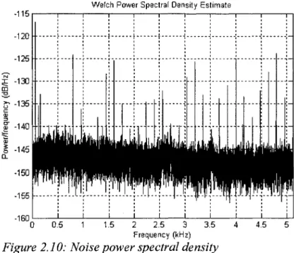
Additionally, a Power Spectral Density (PSD) estimate of the noise is shown in Figure 2.10. The PSD estimate is computed using Welch's method of averaging windowed periodograms. There are several frequency components in the spectrum that are not accounted for by white Gaussian noise. The frequency components at 800Hz and 1600Hz may be coupled from the RN-41 as these match the Bluetooth frequency hopping

intervals. The large spike at low frequencies is 60Hz noise. The other frequency components are likely coupling from the other electronics, but the exact source is unknown.

Welch Power Spectral Density Estimate

-115 I 1 1 1 1 1 1 1 1 1 1--120 i i- f I } \ \ -i -i !125 \ \ J j | j \ I i j -x -130 \ \ j ; ; ; -jl- \- —-j -;-OD i i ! : i ! : : i

&135J4j !T!iM JJH4! j

-Figure 2.10: Noise power spectral density

The RMS level of the noise is 3.498uV. This level is higher than the 2.095uV expected by theory. Part of this noise may be due to high frequency noise aliasing to lower frequencies, as discussed in Section 2.4.1. Converting this voltage into a torque

gives 0.1010 N • m . This level meets the design requirement of less than 0.15 N • m of noise.

2.4.3 Transmitter Latency

The latency between the capturing of a piece of data and its reception by the receiving software is determined by many factors, both in hardware and in software. To measure the one-way latency from the transmitter to the receiver is difficult without precise timing on both sides. If one assumes that the one-way latency is half of the round trip latency, then one can take advantage of the fact that measuring the round-trip latency is relatively easy in a bidirectional communications setting such as Bluetooth.

Round-Trip Latency 140 120 100 80 60 40 20

Round-Trip Latency Histogram

LI

J

0 200 400 600 800 1000

Sample

Figure 2.11: Round-trip latency of 1000 samples

40 50 60 70

Latency (ms)

80

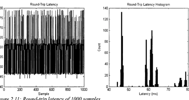
To measure the round-trip latency with Smart Tool Holder, one simply sends a message from the PC and measures the time it takes to receive the reply. The PC can send a series of messages to get a better representation of the latency. The latency of 1000 messages and a histogram of these latencies is shown in Figure 2.11. This method of measuring latency does not account for the delay in the A/D converter. The delay

introduced by the converter, however, is less than 15 microseconds and can be reasonably ignored.

The average latency for these samples was 58.5ms, with a spread of 35.3ms. The standard deviation was 9.5ms. The histogram shows that the latency was not uniformly distributed, but rather tended to cluster around certain values. The exact cause of this phenomenon is unknown, but may be due to buffering of the data in the operating system, or the spacing of the Bluetooth transmission windows.

The latency of the transmitter meets the design requirement of 100ms even without the assumption of round-trip latency being twice the one-way latency. It should be noted, however, that this test only shows that the latency meets the design

requirements for the test conditions, not that it necessarily does in all situations. Other PCs may have different latencies due to software or driver variations. To ensure that the latency meets the design requirements, one would have to use the device in conjunction with a PC utilizing a real-time operating system that can provide guarantees about timing. 2.4.4 Battery Discharge Characteristics

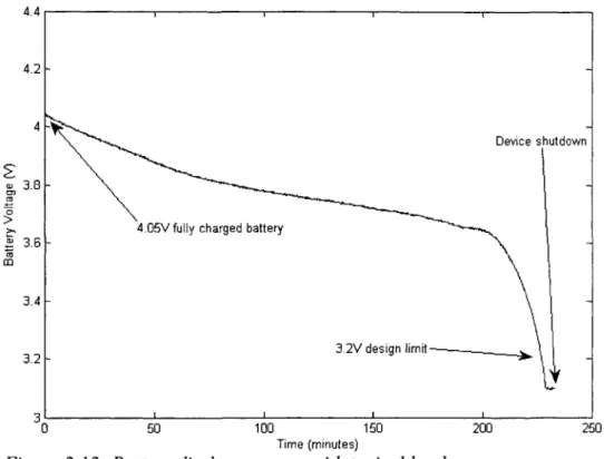
The discharge test monitored the voltage of the battery on the Smart Tool Holder under typical loading and transmitted the voltages to a PC. The discharge test puts the Smart Tool Holder software into battery monitoring mode, where instead of sending the torque value from the external A/D converter, it instead sends the voltage from the internal A/D converter connected to a resistor voltage divider across the battery (the electrical schematic in Appendix A gives full details on this voltage divider). The battery voltage can then be received by the PC instead of the torque data with no software

changes. In this way, the loading will be similar to the loading experienced during normal usage. The test used a freshly charged battery.

3 1 i i i i I

0 50 100 150 200 250

Time (minutes)

Figure 2.12: Battery discharge curve with typical load

The results of the discharge test are shown in Figure 2.12. It took 227 minutes to reach the design limit of 3.2V. The device continued to function for another 5 minutes before the lack of voltage caused the microcontroller to cease operations.

This test indicates that the selected battery can power the device for a much longer period of time than the stipulated hour. Additionally, it is possible to include another battery in the design, effectively doubling the run time.

2.4.5 Battery Charge Time

The charge test was to take batteries discharged to various levels, and measure the length of time it took the charging circuitry to fully charge them. Three tests were

performed, each at a different initial voltage. The results are summarized in Table 2.3. Test#

1 2 3

Initial Battery Voltage (V) 3.215V 2.833V 1.937V

Charging Time (min) 88 80 93

Table 2.3: Battery charge times

While there is significant variation in the initial voltages, the charging times are relatively similar. The conclusion for the charging time is that it exceeds the design requirements. Even a completely empty battery can be fully charged in less than two hours.

2.5 Summary

Every design requirement, with the exception of the aliasing requirement, was met. Even though aliasing was present, it should only manifest itself as additional noise in the spectrum. The noise was experimentally verified as being 0.1010 N-m . Though the noise was higher than expected, it still met the design requirement of being less than

0.15N-m.

The next chapter, Chapter 3, discusses the use of a new file format for storing experimental setup alongside cutting data for the purposes of archival. Readers interested solely in the Smart Tool Holder may skip ahead to Chapter 4 for a discussion of the applications of the Smart Tool Holder.

CHAPTER 3

INFORMATION TECHNOLOGY

3.1 Introduction

In machining research, data is acquired from a variety of sensors, analyzed, and then stored for later reference. In many situations, however, the data is never again used because either the particular experiment's exact setup has been forgotten or because the definition of the data format has changed (e.g. column 5 currently represents power but previously held audio information instead). This leads to cutting tests duplicating

previous results, a waste of time and resources. Additionally, since the second experiment has no more documentation than the first, it is likely that future testing will again

duplicate the original experiment.

The Extensible Markup Language (XML) [W3C XML] has successfully been used to facilitate data storage and exchange in machining systems through efforts such as MTConnect [MTConnect] and NCML [Ryou 2001, Ryou and Jerard 2001, Schuyler 2005, Jerard and Ryou 2006]. MTConnect focuses on collecting machine status from devices created by different vendors in a distributed environment. NCML was developed to provide a standard format for describing a part to be machined. These efforts have not, however, been targeted at the problem of annotating sensor data. While MTConnect can be used to collect data from low-bandwidth sensors, it is limited in what annotations can

be added. Using XML to annotate sensor data, has, however, been researched in other fields. WellLogML was developed to hold well logs for the oil industry [WellLogML]. Similarly in the medical field, ecgML was developed to hold electrocardiogram data [Wang, et al. 2003]. While neither of these solutions can be applied directly to machining, the principles and ideas that they are based on can be reused to create a machining sensor data storage format.

To be useful, a data format needs to be able to describe its contents explicitly and have the ability to change the format without invalidating older documents. Without these features, older data may become unreadable due to format changes. Additionally, the files should contain as much information as possible about the cutting experiment, so that the contents can remain useful after the specifics have been forgotten by the experimenters.

Because different research groups focus on describing different portions of the experimental setup, the format cannot be too specific about what must be present. Instead, it should provide a flexible method for research groups to add the information that is important for their research, without worrying about specifying the irrelevant data a broad format would impose.

XML was chosen for for the basis of the new file format because it can describe its contents explicitly and allows changes to the format that won't render older files useless. Because of its ubiquitous nature, many software tools and libraries already exist for reading and writing XML documents, saving considerable programming time during the development of analysis tools.

3.2 XML Schema

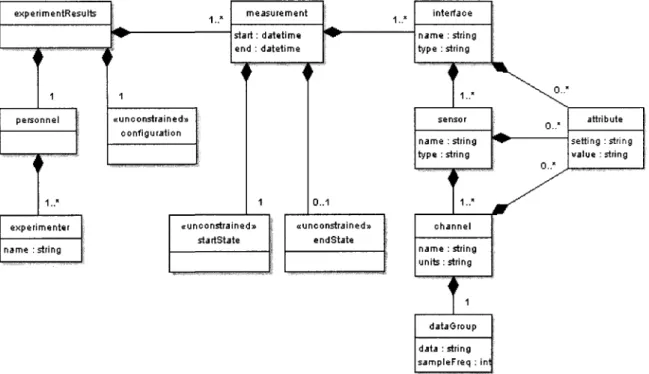
XML formats are each defined by an XML schema [W3C XML Schema]. A schema specifies the layout of the data within the files, and what data is optional or required. A graphical representation of the schema for the experiment results format is shown in Figure 3.1, and the full schema definition is contained within Appendix D. On the figure, the lines with diamonds represent a "is contained within" relationship. For example, an experimenter node is contained within & personnel node. An experimenter node cannot be located outside ^personnel node. The numbers on the lines represent the cardinality of the relationship. A " 1 " means that the node is required to exist. A "0.. 1" means that the node is optional, but there cannot be more than one instance. A "0..*" means there can be any number of nodes, including none. A " 1 . . * " means that at least one node is required to exist, but there may be any number of additional nodes.

e x p e r i m e n t s

T~

The contents of the blocks in Figure 3.1 represent required attributes of the nodes. For example, an experimenter node is required to have a name, and a channel node is required to have both a name and a unit. The «unconstrained» marked on

configuration, startState and endState symbolize that the contents of those nodes are not

defined by the schema, but rather are left up to each research group to determine for their specific needs.

Each of the nodes is described in detail:

• experimentResults: this is a container for everything else in the file, since XML only allows a single top-level node.

• personnel: this node is just a container for the experimenter nodes.

• experimenter: each of these nodes contain the name of a person associated with running the experiment. At least one experimenter node is required per file. • configuration: this unconstrained node holds setup information relevant to the

entire experiment. For example, the identity of the CNC machine would go in here, since that doesn't change while performing an experiment.

• measurement:concGptua\\y, a measurement is a continuous stream of data from various sensor inputs over a short duration. If continuous data over a long duration is required, the data can be split across multiple measurements. • startState: this unconstrained node holds setup information known at the

beginning of the measurement, such as the bed position, tool type, or the G-code line being executed.

has changed since the beginning of the measurement, such as bed position. Each measurement should be short enough so that any change between startState and

endState can be easily understood or interpolated.

• interface: this is a container for sensors. Conceptually, an interface is an A/D converter, or some other connection between sensors and the recording computer. • sensor: this represents a physical sensor, such as a microphone or dynamometer.

Each sensor contains at least one channel. For example, a triaxial accelerometer would contain a three channel nodes representing the different axes of

measurement.

• channel: this is a single independent stream of data from a sensor. Each channel holds a single dataGroup for its captured data.

• dataGroup: this node holds whitespace separated data points, sampled at the specified sampling frequency.

• attribute: these nodes can be used to annotate the interface, sensor, and channel nodes with specific information, such as the port on the A/D converted used to sample the data.

An example file conforming to this schema is shown in Appendix E.

The UNH Smart Machining System Platform [Xu 2007] was extended to record sensor data in the XML format and included annotations such as axial depth, spindle speed, radial engagement, and part program line number. The open source Xerces-C++ XML Parser [Xerces-C++] was utilized by the program to create the XML output.

3.3 MATLAB Toolbox

To facilitate analysis of collected machining data, a MATLAB toolbox was created for reading the contents of the XML data files with the schemas described in Section 3.2. The bulk of the toolbox was written in the Java programming language because of the extensive XML parsing functionality that it provides. The Java portion has all of the parsing functions and unit transformations. The unit transformations are done using the JSR-275 Measures and Units library [JSR-275]. The Java portion of the toolbox also provides a Graphical User Interface (GUI) that allows a user to load files and select specific channel nodes to examine. Each of the analysis tools is written in MATLAB "m code". They call specialized routines to handle the conversion between the Java code and

P

Be E* !»»

D & H #

Insert Tool* De^ug Qe*kep Window tJefc

I -w New Subplots :: Q 2D Axes • l ^ . 3D Axes • \w. Annotations . * ^ Dotfcle Arrow ' ^ Text Arrow i T Text Box :. Q Rectangle :; O E » P S O

Lata fasm channel l~x

r

1

i^3 Mowig W«Tdow FFT E i FFT

a

[ B U)w Frequency FFT S FFT

m code. Each of the analysis tools is written in m code, and calls the Java functions to load the data. Specialized routines transfer the data between the Java section of the toolbox and the m code section of the toolbox.

One of the tools contained in the MATLAB Toolbox is the Fourier Analysis Tool, which allows one to inspect both time and frequency domain representations of the channel data (see Figure 3.2). It uses the spindle speed annotation from the XML file to show the spindle frequency on the frequency domain plots, and provides an option to the user to add the spindle component to the time domain plot. All plots generated by the

Hr>.'i-o->"_ _ " J ' ' •

File Edit View Insert Tools Desktop Window Help

D'C* y © T fe ^ o T o W S : • m n

S 1.4

s

- i

• I

f

V

V ^ ?

u

V

:

MATLAB Toolbox can be edited using the standard MATLAB tools and commands. For example, the figure axes can be relabeled to be more specific to the experiment. This provides maximum usability to the user while still allowing simple usage.

Another tool, the Average Plotting Tool, allows one to take multiple channels of data and plot their average. This is useful for visualizing the average power or force for different cutting conditions. An example plot is shown in Figure 3.3, where average force in the X axis is plotted versus the line number of the part program. For plotting

mechanical power from the electrical power sensor data, the tool provides the user an option to subtract the tare power (as recorded in the XML file) and multiply by the motor efficiency. Power sensors are discussed further in Section 4.4. The Average Plotting Tool also provides the user with the option of plotting either the arithmetic mean or the Root Mean Squared (RMS) average. The arithmetic mean is given by:

x

i-\

arithmetic mean * r = T T 2 > / > C3-1)

where x, is the /th data point, and N is the total number of data points. The RMS average is given by:

X RMS

A^t*-

<">

1=0

The RMS average is useful with signals that have zero mean, such as the sinusoids found in AC voltage and current.

The Ktc, Kte Regression Tool is used to find the tangential coefficients K,c and Kle

[ H - • - ; . . : . - • • • • • • • • • ' • - • • • • File Edit View Insert Tools Desktop Window Help

• csyaife G ^ ^ ® j « : o i B [ i ° Q

Figure 3.4: Example usage of the Ktc, Kte Regression Tool

from several cuts as its input, and plots PIAC (average mechanical power per swept

contact area per time) versus havg (average chip thickness). This provides a way to

estimate the force due to the chip thickness in a manner independent of cutting geometry. Each cut becomes a single data point on the plot. The slope of the trend line of these points is K,c and the intercept is K,e (see Figure 3.4).

Further capabilities of the MATLAB Toolbox are described in Appendix F. 3.4 Summary

The XML based data files were used to hold the data from the wear tests performed in [Cui 2008] and [Javorek 2008], indicating that the file format is, at minimum, usable for controlled testing environments. The MATLAB Toolbox helped to simplify many repetitive analysis tasks.

CHAPTER 4

APPLICATIONS OF THE SMART TOOL HOLDER

4.1 Introduction

A high-bandwidth torque sensor like the Smart Tool Holder has direct application to the study of regenerative chatter. Regenerative chatter is a phenomenon in milling where surface "waviness" from small vibrations in the cutting tool left from the last tooth pass interfere with the vibrations from the current tooth pass, yielding even more

waviness and vibration. This positive feedback can quickly lead to workpiece damage as the tool vibrations exceed the tolerances. Additionally, the high forces during chatter can destroy cutting tools and cause increased wear on spindle bearings. Chatter only occurs when the vibrations are out of phase with the vibrations from the last tooth pass, causing variation in the chip thickness. This means that chatter is dependent on the the tooth passing frequency (based upon the spindle speed and number of cutting teeth) and the chatter frequency. The chatter frequency is based upon the system properties (i.e. mass, stiffness and damping). The chatter frequency can be close to the natural frequency of the spindle and the tool, but may be influenced by the natural frequency