Energy efficiency\u27s role in a zero energy building: simulating energy efficient upgrades in a residential test home to reduce energy consumption

ENERGY EFFICIENCY‟S ROLE IN A ZERO ENERGY BUILDING:

SIMULATING ENERGY EFFICIENT UPGRADES IN A RESIDENTIAL TEST HOME TO

REDUCE ENERGY CONSUMPTION

by

Andrew Frye

A thesis submitted in partial fulfillment of the requirements for the degree of

M.S. Mechanical Engineering

University of Tennessee at Chattanooga

UNIVERSITY OF TENNESSEE AT CHATTANOOGA

ABSTRACT

Energy Efficiency‟s Role in a Zero Energy Building: Simulating Energy Efficient Upgrades in a Residential Test Home to Reduce Energy Consumption

by Drew Frye

Chairperson of the Thesis Committee: Dr. Prakash R. Dhamshala College of Engineering

With the steady rise in power consumption, automobile usage, and industrial production worldwide for the past century, countries have realized that meeting these ever-growing energy demands could potentially devastate the environment. In the United States, generating electrical power constitutes the largest source of carbon dioxide

emissions and the majority of this power is used to electrify buildings both in the commercial and residential sectors. It is estimated that 21% of all electrical power generated in the United States is consumed by residential buildings. To reduce the total amount of electricity that need be generated (and therefore, the amount of pollution) governments have invested heavily into energy efficiency research especially in the major power consuming sector of residential buildings. The ultimate goal of energy efficient measures is to cut the power consumption of a building enough that all of the energy needs can be met by an on-site renewable energy system such as photovoltaic solar panels. This would result in what many call a “zero energy building.” This paper quantitatively investigates the effectiveness of potential energy efficient upgrades in a residential home through various building energy simulation techniques including the computer building load and energy requirement software entitled “Transient Analysis of Building Loads and Energy Requirements” or TABLER. Energy savings from energy efficient upgrades were investigated in the areas of residential lighting, building envelope infiltration mitigation, advanced insulating materials, advanced window technologies, electrical plug-load reduction strategies, and energy efficient appliance options. Results of simulations show significant energy savings for various energy efficient upgrades can be achieved either by a reduction in the electrical power consumed directly by the device (lighting, electronics, and appliances) or by a reduction in power consumption of the home heating, ventilation, and air-conditioning (HVAC) equipment used to remove or add heat to the conditioned space throughout the year. The effectiveness of individual upgrades as compared to the total investment required to implement them is a matter of opinion slanted by whether energy conservation or return on investment is the ultimate goal.

TABLE OF CONTENTS

List of Tables viii

List of Figures xi

List of Symbols xv

Chapter 1 Introduction 1

1.1 Thesis Research Purpose 5

Chapter 2 Residential Test House 7

2.1 Floor Plan / Home Design 7

2.2 Heating Ventilation and Air-Conditioning (HVAC) System 13

2.3 Typical Power Consumption of Home 18

Chapter 3 Lighting 23

3.1 Light Efficiency and Efficacy 24

3.3 Lighting Energy (Electricity and Thermal) Loads 32

3.3 Baseline Lighting Simulation Procedure 34

3.4 Lighting Results / Savings Estimates 40

3.5 Daylighting Techniques 45

3.6 Brief Remarks on Lighting 54

Chapter 4 Infiltration Mitigation 56

4.2 Infiltration Simplified Models – LBNL Model 69

4.3 Infiltration Energy Loads 73

4.4 Baseline Simulation Procedure 75

4.5 Energy Efficient Upgrades for Infiltration Mitigation 96

4.6 Infiltration Mitigation Energy Efficient Simulation / Results 88

4.7 Brief Remarks on Infiltration 93

Chapter 5 Advanced Insulation 94

5.1 Insulation Basic Concepts and Terminology 94

5.2 Insulation Simulation Procedure 104

5.3 Baseline Simulation of Insulation System 112

5.4 Energy Efficient Insulation Upgrades 115

5.5 Energy Efficient Insulation Simulation Results 121

5.6 Brief Remarks on Insulation 123

Chapter 6 Advanced Windows 125

6.1 Windows Basic Concepts and Terminology 125

6.2 Advanced Windows 128

6.3 Importance of Southern Window Over-Hangs 130

6.4 Window Baseline Energy Simulation 137

6.5 Window Energy Efficient Upgrades 140

6.6 Energy Efficient Window Upgrade Energy Simulation 142

Chapter 7 Plug Loads – Appliances and Electronics 150

7.1 Plug Load Basic Concepts and Terminology 150

7.2 EnergyStar® Products 152

7.3 Test House Plug Loads and Appliance Loads 159

7.4 Major Appliances 165

7.5 Brief Remarks on Plug Loads 175

Chapter 8 Total Building Energy Simulation 178

8.1 Baseline Total Building Energy Simulation 181

8.2 Total Building Energy Efficient Upgrades 183

8.3 Brief Remarks on Total Building Energy Simulation 194

Chapter 9 Solar Power Generation 197

9.1 Solar Power Generation Simulation 205

Chapter 10 Conclusions and Recommendations 209

References 214

Appendix A Cooling Load Factors (CLF) for Lighting 219

Appendix B Zone Types and Zone Parameters for CLF Values 221

Appendix C Energy Efficient Lighting Conditions for Simulation Sets 222

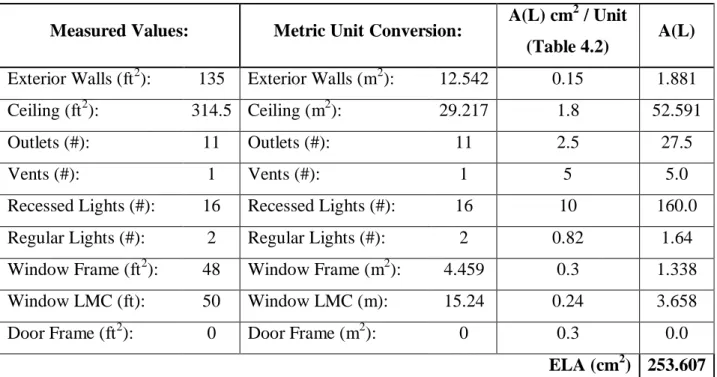
Appendix E Effective Leakage Area Calculations for Whole Test House 230

Appendix F Air Changes per Hour Computer Code: ACHcalc.m 235

LIST OF TABLES

Table 2.1: Cooling Performance Characteristics of Payne 15 PH12 036-G Split-System Heat Pump

Table 2.2: Heating Performance Characteristics of Payne 16 PH12 036-G Split-System Heat Pump

Table 2.3: Test Home Utility Information 22

Table 3.1: Incandescent Light Bulbs Commercially Available 29

Table 3.2: Fluorescent Light Bulbs Commercially Available 30

Table 3.3: LED Lights Commercially Available 31

Table 3.4: Base-Line Energy Simulation Data 39

Table 3.5: Important CFL Simulation Results 42

Table 3.6: Important LED Simulation Results 43

Table 3.7: Important Combination LED & CFL Simulation Results 45

Table 3.8: Important Simulation Results 54

Table 4.1: Percentage of Air Leakage Area by Building Components 64

Table 4.2: Sample of Component Effective Air Leakage Area 65

Table 4.3: Stack Coefficient Cs 71

Table 4.4: Local Shielding Classes 71

Table 4.5: Wind Coefficient Cw 72

Table 4.6: Sample Calculated Leakage Area for the Living Room

of the Test Home 76

Table 4.7: Energy Audit and CEC Recommended Upgrades 87

Table 4.8: Simulation Results and Savings from Infiltration

Mitigation Upgrades 93

Table 5.2: ORNL Insulation Recommendations 102

Table 5.3: Exterior Wall U-Factor Calculations 107

Table 5.4: Floor U-Factor Calculations 108

Table 5.5: Main Room Ceiling U-Factor Calculations 109

Table 5.6: Bedroom Roof R-Value Calculations 109

Table 5.7: Bedroom Ceiling R-Value Calculations 110

Table 5.8: TABLER Solid Envelope Inputs for Insulation

Energy Simulations 111

Table 5.9: Major Construction Project Cost Breakdown 120

Table 5.10: Review of Test Home Insulation Upgrades 120

Table 5.11: Insulation Upgrade Simulation Results 121

Table 5.12: Review of Insulation Simulations and Savings 124

Table 6.1: Full Frame R-values and U-factors for Typical Windows 127

Table 6.2: Sample of Various SeriousWindowsTM Advanced Windows 129 Table 6.3: 3M Window Sun Coating Performance Characteristics 129

Table 6.4: Sustainable Design‟s Over-hang Annual Analysis

Online Tool Results for Typical Pitched Southern Over-hang.

Percentage of Direct Sun Incident on these Windows 133

Table 6.5: Over-hang Design Recommendations for Chattanooga 136

Table 6.6: Actual Test Home Window Information 137

Table 6.7: SeriousWindowsTM Energy Efficient Test Home

Window Upgrades Test 1 141

Table 6.8: 3M CM40 Window Coatings Upgrade Test 2 141

Table 7.1: Energy Star Requirements for Clothes Washing Machines 153

Table 7.2: EnergyStar® Specifications for Dishwashers 154

Table 7.3: EnergyStar® Specifications for Refrigerators and Freezers 156

Table 7.4: EnergyStar® Requirements for Televisions Based on

Viewable Screen Area 157

Table 7.5: EnergyStar Computer Specifications 158

Table 7.6: EnergyStar Monitor Specifications 158

Table 7.7: Power Measurements of Test House Electronics and Appliances 160

Table 7.8: Total Annual Power Consumption and Expenditure Estimation 162

Table 7.9: Annual Vampire Electronic Loads Broken Down into

Standby and OFF Modes 164

Table 7.10: Cooking Methods and Power Consumption / Cost 173

Table 7.11: Electric vs. Gas Cooking Appliances 174

Table 7.12: Review of Plug Loads -Electronics and Appliance

Important Information 177

Table 8.1: TABLER Inputs for Baseline, Whole Building Energy

Simulation 180

Table 8.2: Baseline Total Building Energy Simulation Results 181

Table 8.2: TABLER Inputs for Best Case Energy Efficient Whole

Building Simulation 185

Table 8.3: Best Case Energy Efficient Total Building Simulation Results 186

Table 8.3: TABLER Inputs for Cost Effective Energy Efficient

Upgrades Simulation 190

Table 8.4: Cost Effective Energy Efficient Whole Building Simulation Results 191

Table 8.5: Whole Building Energy Efficient Upgrade Simulation Results 194

LIST OF FIGURES

Figure 1.1: Carbon Dioxide Emissions by Energy Source from Annual

Energy Review 2009 2

Figure 1.2: Department of Energy U.S. Primary Energy Consumption

End-Uses 2006 4

Figure 2.1: Conditioned Space Dimensioned Floor Plan 8

Figure 2.2: North Face of Test Home 9

Figure 2.3: South Face of Test Home 9

Figure 2.4: East Face of Test Home 10

Figure 2.5: West Face of Test Home 10

Figure 2.6: Window Over-hang on Southern Windows 11

Figure 2.7: Southern Roof Tilt for Solar Systems 12

Figure 2.8: Average Monthly Home Electricity Consumption 19

Figure 2.9: Average Monthly TVA Average Fuel Cost Adjustments 20

Figure 2.10: Average Monthly Natural Gas Consumption 21

Figure 2.11: Average Monthly Utility Expenses for Electricity and

Natural Gas 21

Figure 3.1: Solartube® Technologies Sun Tubes 47

Figure 3.2: Solartube® 160DS Light Output for February 5th 49 Figure 3.3: 60 Watt Incandescent Light Bulbs Replaced on February 5th 49 Figure 3.4: Solartube® 160DS Light Output for July 4th 50 Figure 3.5: 60 Watt Incandescent Light Bulbs Replaced on July 4th 51 Figure 3.6: Solartube® 160DS Monthly Average Lumen Output

During Daylight Hours 52

Light Bulbs Replaced 52

Figure 3.8 Energy Consumption Due to Lighting Conditions 55

Figure 4.1: ACH New Construction 58

Figure 4.2: ACH Low-Income Housing 58

Figure 4.3: Pressure Differences Caused by Stack Effect in Heating Season 61

Figure 4.4: Average Monthly Airflow Rate (Q) into/out of the Test House 79

Figure 4.5: Home Average Monthly ACH 79

Figure 4.6: Average Monthly ACH values with Data Range for Test house 80

Figure 4.7: Breakdown of Monthly Thermal Loads due to Air Infiltration 82

Figure 4.8: Heating and Cooling HVAC Power Consumption Due

to Infiltration 85

Figure 4.9: Utility Expenses Due to Infiltration 85

Figure 4.10: New Average Monthly Airflow Rate (Q) into/out of the

Test House 89

Figure 4.11: New Home Average Monthly ACH 89

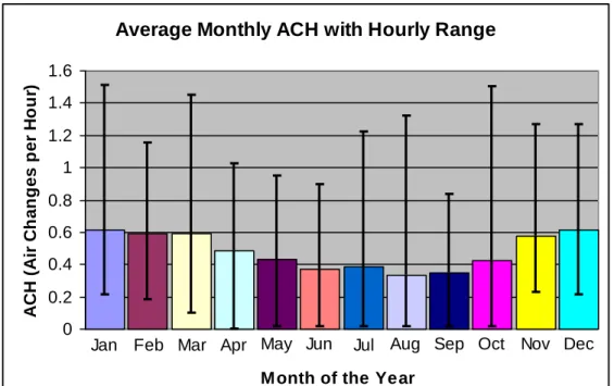
Figure 4.12: New Average Monthly ACH values with Data Range for

Test house 90

Figure 4.13: Breakdown of New Monthly Thermal Loads due to Air

Infiltration 91

Figure 4.14: New Heating and Cooling HVAC Power Consumption

Due to Infiltration 91

Figure 4.15: New Utility Expenses Due to Infiltration 92

Figure 5.1: Monthly Heating and Cooling Loads through Insulation Systems 112

Figure 5.2: Monthly HVAC Power Consumption from Heating

and Cooling Loads Transmitted through Insulation Systems 114

Transmitted through Insulation Systems 114

Figure 5.4: New Space Heating and Cooling Loads from Heat Loss and Heat Gain Through Upgraded Wall Insulation

Structure (R-5 Sheathing and R-15 Cavity) 123

Figure 6.1: Solar Heat Gain through Southern Windows 131

Figure 6.2: Sustainable Design‟s Over-hang Annual Analysis

Online Tool Inputs 133

Figure 6.3: Southern Window Solar Heat Gain with and

without Window Over-hangs 135

Figure 6.4: HVAC Power Consumption to Remove the Difference

in Solar Heat Gain with and without Southern Window Over-hangs 135

Figure 6.5: Comparison of Heating/Cooling Loads with and without Windows 138

Figure 6.6: Baseline HVAC Power Consumption for Heating/Cooling

Loads through Insulation and Windows 138

Figure 6.7: Baseline Utility Expenses for Heating/Cooling

Loads Through Insulation and Windows 139

Figure 6.8: HVAC Power Consumption with New, Energy Efficient Windows Compared to Baseline Consumption for

Heating/Cooling loads seen through the Windows and Insulation 142

Figure 6.9: Utility Expenses for Heating/Cooling Loads Through

Insulation and Upgraded Windows 144

Figure 6.10: HVAC Power Consumption with 3M Solar Coatings Compared to Baseline Consumption for Heating/Cooling

loads seen through the Windows and Insulation 145

Figure 6.11: Utility Expenses for Heating/Cooling Loads Through

Insulation and Current Windows with 3M CM40 Solar Coatings 146

Figure 6.12: Breakdown of the HVAC Power Consumption for the Heating/Cooling Loads Attributed to Heat Gain Through the

Windows and Walls 148

Figure 6.13: Expected Total Annual Utility Expenses to Mitigate the Heating/Cooling Loads Attributed to Heat Gain Through

the Windows and Walls 149

Figure 7.1: Average Measured Hourly Refrigerator Power Usage 167

Figure 7.2: Measured Refrigerator Power Consumption 167

Figure 7.3: Geoexchange Graph of Power Consumption (kWh)

Old and New Refrigerator 168

Figure 8.1: Baseline Electricity Consumption Breakdown by End-Use 182

Figure 8.2: Baseline Utility Expenditures by End-Use 182

Figure 8.3: Electricity Savings of Best Case Energy Efficient Upgrades 187

Figure 8.4: Best-Case Electricity Consumption Breakdown by End-Use 188

Figure 8.5: Best-Case Estimated Utility Expenditures by End-Use 188

Figure 8.6: Electricity Savings of Cost Effective Energy Efficient Upgrades 192

Figure 8.7: Cost Effective Electricity Consumption Breakdown by End-Use 193

Figure 8.8: Cost Effective Estimated Utility Expenditures by End-Use 193

Figure 8.9: Compare Whole Building Energy Efficient Upgrades with

Baseline End-Uses 195

Figure 9.1: Photovoltaic and Concentrating Solar Power Resources in U.S. 198

Figure 9.2: Important Solar and Orientation Angles for Solar

Power generation Evaluation 202

Figure 9.3: PV System Sizing Based on Home Energy Consumption

LIST OF SYMBOLS

TC Total Cooling Capacity SC Sensible Cooling Capacity Ta Ambient Air Temperature

Wc Cooling Mode Heat Pump Electrical Power Consumption THhp Total Heat Pump Capacity

Wh Heating Mode Heat Pump Electrical Power Consumption Ful Light use Factor

Fsa Light Special Allowance Factor CLFel Lighting Cooling Load Factor

r Reflectance

t Light Transmittance ILLDN Direct Normal Illuminance ILLDH Diffuse Horizontal Illuminance I Air Exchange Rate

Q Volumetric Flow Rate

V Volume

Δp Pressure Difference between indoor and outdoor po Static Pressure

pwind Wind Pressure pi Interior Pressure ρ Density g Gravitational Constant Cw Wind Coefficient Cs Stack Coefficient AL Leakage Area

Ac Building Leakage Area Cp Specific Heat

W Humidity Ratio

R Resistance

U Overall Heat Transfer Coefficient It Total Solar Load

Idirr Direct Solar Radiation Idiff Diffuse Solar Radiation Iref Reflected Solar Radiation

Idiff,horiz Diffuse Horizontal Solar Radiation θ Angle of Incidence

β Surface Tilt

n Julian Day Counter δ Declination Angle Et Equation of Time

Lst Longitude of Standard Time Lloc Longitude of Location

ώ Angle Hour

tsol Solar Time α Altitude Angle

φ Latitude

Ζ Zenith Angle

χ Solar Azimuth Angle

ε Surface Azimuth

Azs Surface Asimuth to the North Pmax Maximum Power

Voc Open Circuit Voltage Vmp Voltage at Maximum Power Isc Short Circuit Current

Imp Current at Maximum Power

Chapter 1

Introduction

With the steady rise in power consumption, automobile usage, and industrial production worldwide for the past century, countries have realized that meeting the growing energy demands of the public could potentially damage the environment [1]. Scientists and engineers have been examining the environmental impact of pollution for years; and dangerous trends of high contamination levels have been observed

contributing to a host of environmental problems collectively termed “global climate change,” or “global warming.” In December 2009, political leaders, scientists, engineers, and economic/environmental advisors gathered in Copenhagen, Denmark for a

symposium entitled the “United Nations Climate Change Conference.” Here the

implications of impending global climate change were discussed, and limits for noxious emissions, such as carbon dioxide, sulfur dioxide, and nitrogen oxides, for countries (individually or collectively) were examined. From these talks, a document entitled the “Copenhagen Accord” was drafted by several countries including the United States, China, Brazil, and India. This document basically states that global climate change is one of the greatest challenges of present day and that actions should be taken to mitigate contributing factors such as carbon dioxide emissions. One hundred and thirty eight countries have signed this agreement pledging to examine different ways of reducing emissions in their respective countries. Countries are asked to “spell out” by the

following year (2010) their promises and plans for cutting carbon emissions by 2020 1[1]. Limiting dangerous emissions, such as carbon dioxide, will be essential to

combating global climate change. A stark look at major pollution contributors in each country will reveal potential opportunities for improvements. According to the U.S. Energy Information Administration (EIA), 39% of anthropogenic (caused by humans) carbon dioxide emissions in the United States in 2002 were attributed to the combustion of fossil fuels for the generation of electricity [2]. A breakdown of carbon dioxide emissions by energy source taken from the EIA‟s Annual Energy Review of 2009 is shown in Figure 1.1.

Figure 1.1: Carbon Dioxide Emissions by Energy Source from Annual Energy Review 2009 [2]

In 2009, 74% of the electricity produced in the United States came from

environmentally harsh fossil fuels [2]. Of that number, 54% of the country‟s electricity was generated by coal combustion power plants making them the country‟s single largest contributor to air pollution [3]. Many scientists and engineers have been working

towards generating power in more environmentally “friendly” ways by utilizing nuclear power, hydrostatic power generation, and a multitude of renewable energy sources, resulting in an engineering task of massive scale and economic investment.

While power generation technologies are examined and improved with regards to carbon emissions, a major push to examine how to reduce the amount of power that utilities must ultimately produce has been underway for many years now. This push is known as energy conservation. Energy conservation is defined as “efforts made to reduce energy consumption.” Sometimes the term energy efficient is used as a substitute for energy conservation, but there is a subtle difference in definition. Being energy efficient is defined as “efforts made to reduce the amount of energy required to provide the same products and services.” This may seem like a meaningless distinction; however,

For example, energy conservation could simply be the practice of turning off half of the lights in a room when watching television to reduce the amount of energy the room is consuming. On the other hand, this would not be considered energy efficient because the “same products and services” (the amount of light in the room) is not the same as before. Instead, energy efficient light bulbs could be installed that use a fraction of the electricity as traditional light bulbs while providing the same amount of light in the room as before. This would be known as being energy efficient.

Despite the terminology differences, to effectively reduce the amount of power that utilities must ultimately produce, an assessment of the destination, or “end-use” of this energy must be completed. In the United States, 36% of the electricity produced is consumed by the residential market (highest percentage by sector) [4]. In a broader energy discussion (all energy types not just electricity but natural gas and other forms of energy as well); the Department of Energy (DOE) estimates that 39% of the primary energy sources in the U.S. are consumed by commercial and residential buildings [5]. Figure 1.2shows the DOE break down of the U.S. primary energy consumption sectors (Industrial, Transportation, and Buildings) and the primary energy end-uses of the “Buildings” (commercial and residential) sector in 2006.

According to the DOE energy consumption breakdown, 21% of U.S. energy (electricity, natural gas, etc) is consumed by the residential sector, while 18% is

consumed by commercial buildings. This segment of energy usage has been targeted by many industry leaders, government agencies (DOE and EIA), and conservation activist as a possible area where great improvements and energy savings could be made by

integrating new energy efficient technologies [5].

Further investigation into this DOE energy end-use study reveals that the top energy consuming applications in the residential sector are heating and cooling, lighting, and appliances/electronics.

Figure 1.2: Department of Energy U.S. Primary Energy Consumption End-Uses 2006 [5]

According the Department of Energy, 42% of a home‟s total energy consumption is directed towards heating and cooling (28% and 14%, respectively) needs [5]. The DOE estimates that 56% of the electricity demand for a typical U.S. home comes from heating and cooling needs. This value is of course geographically contingent. According to Austin Energy (out of Austin, Texas), during summer months the air conditioning demands for a typical Austin home will be 60 – 70% of the total electrical demand for that home [6]. Since heating and cooling represent the largest area of energy

consumption for a typical U.S. home, there is a great potential for energy savings by utilizing energy efficient heating/cooling systems such as high efficiency heat pumps, split energy systems, and other high efficiency HVAC units.

Making sure a home has an energy efficient HVAC (heating, ventilation, and air conditioning) system is just a small step in reducing the buildings‟ heating and cooling energy consumption. A large, sometimes over-looked, aspect of mitigating the heating and cooling energy requirements of a home is limiting the unintentional heat gained during the summer and heat lost during the winter months to the outside environment.

Limiting the air exchange (infiltration) of outside ambient air with indoor conditioned air, utilizing advanced window technologies, and making use of advanced insulations can reduce the heating and cooling loads of a typical building.

1.1 Thesis Research Purpose

This thesis is intended to identify, understand, simulate, and evaluate energy efficient upgrades related to residential (1) lighting, (2) infiltration mitigation, (3) advanced insulation, (4) advanced windows, and (5) plug and process loads. From simulations potential energy and utility savings for these upgrades will be examined for a specific test home in hopes of creating a zero-energy building in a somewhat cost

effective manner.

According to the Department of Energy, the third largest area of energy

consumption in a typical U.S. home is lighting. This study states that 12% of the total energy a home consumes is used for lighting [5]. Several emerging technologies in the field of advanced lighting techniques have increased lighting efficiency. The energy savings from Compact Fluorescent Lights (CFLs) and Light Emitting Diodes (LEDs) are two emerging lighting technologies which will be presented in Chapter 3 after describing the test home in Chapter 2.

Altogether, heating/cooling, lighting, and appliances/electronics account for about 72% of the energy needs of a typical U.S. home; however, this value can increase wildly depending on the season and geographical location of a home to upwards of 90% [5]. Energy efficient upgrades to infiltration mitigation, insulation, windows, and

appliances/electronics are presented in Chapters 4, 5, 6, and 7, respectively.

It is also indicated in [5] that 18% of the total energy of a typical residential home is consumed by appliances and electronics. This category includes but is not limited to: refrigerators, clothes washing and drying machines, dishwashers, and various electronics such as the television, computer, and other entertainment devices. This thesis will briefly identify potential savings by upgrading to energy efficient appliances and will catalogue the energy consumption of common electronics that are found in a typical U.S. home in hopes of identifying possible areas of energy savings.

Chapter 8 of this thesis combines the individual energy simulations of the preceding chapters into a “whole building” energy simulation and the combined savings of each energy efficient upgraded will be presented. Reducing a building‟s energy requirement is a significant step towards creating what is known as a zero-energy building (ZEB). A ZEB is a structure that over a period of time (usually a year)

consumes as much energy as it produces. Recently, the U.S. government set milestones for new commercial construction that is directed towards all new construction being “zero-energy” by 2030, and all (already built) commercial buildings being retrofit to meet zero-energy criteria by 2050 [5]. Chapter 9 of this thesis presents the potential solar power generation for the residential test home in hopes that combining energy efficient upgrades with renewable solar power generation will lead towards a possible zero-energy building.

The focus of this research is geared towards making energy efficient upgrades to a residential building, but similar techniques and upgrades can be extended to other

business sectors especially the commercial sector to reach the U.S. government commercial milestones.

Chapter

2

Residential Test House

The residential home under investigation in this thesis is located in Ooltewah, Tennessee (Latitude 35.16, Longitude -85.06) which is a suburb situated slightly North-East of Chattanooga, Tennessee. The home was completed 1988 and was custom

designed by the head of the Tennessee Valley Authority Solar Division at that time. The home has since been slightly modified from the original designs adding indoor living area and outdoor decking area. Despite the changes, no structural modifications were made from the original architectural designs.

2.1 Floor Plan / Home Design

The test home has 3 bedrooms and 2 bathrooms in 2,300 square feet of

conditioned, indoor living area predominantly on a single level. The only “second level” space was added as a modification to the original design and made use of free space that was originally attic/storage. This upstairs space is open to the main living area (open windows) and does not have ductwork or ventilation from the main heating and cooling equipment of the home. This means the upstairs space can be lumped into the same heating/cooling area as the main space of the building (can be seen as an extension of dining/living room space). A computer generated drawing of the home floor plan is presented in Figure 2.1. This figure is drawn to scale and shows some important structural dimensions. The open, upstairs space mentioned before is located over the kitchen and laundry rooms. Although the majority of the living floor space is on a single story, the abnormally tall ceiling (nearly 20 feet in some locations) means the home is sometimes considered a two-story structure when viewed from the exterior (the importance of this is explained in the Infiltration section of this report when needed).

The floor plan of this home is what is considered an “open concept” meaning a large portion of the living space is unimpaired by interior walls or partitions. In fact, the living room, dining room, kitchen, back entry way, front entry way, upstairs open space, and hallway are all open to each other with no full interior walls to separate them.

Figure 2.1: Conditioned Space Dimensioned Floor Plan

This accounts for about 59% of the floor living space (~1348 ft2). This open floor plan concept allows unobstructed air flow throughout the majority of the home. The interior walls in this home are un-insulated or have significantly less insulation relative to exterior walls. Because of the lack of internal heat transfer resistance (no interior wall insulation), open floor-plan layout, and relatively simple (approximately square) shape, this home can be considered a “single heating/cooling zone,” and appropriate single zone modeling procedures were used for various sections of this thesis for determining

required heating and cooling building loads.

This home was designed by a particular advocate of solar techniques; therefore, many features of this home make it attractive for both passive and active solar

applications. For a full explanation of these design features, an understanding of the test home orientation and exterior design are needed. Figures 2.2 – 2.5 are pictures taken from the outside of the test home showing the exterior faces of the home in each cardinal direction: north, south, east, and west.

Figure 2.2: North Face of Test Home

Figure 2.4: East Face of Test Home

The home is situated with the “front” facing north (Figure 2.2) and “back” facing south (Figure 2.3). This of course was a strategic decision based on the lot position relative to the street (transportation access) and other natural features (lake/water access). The southern facing portion of the home (Figure 2.3) contains large areas of glass

features in the form of windows and doors. In fact, about 37.7% of the southern facing wall area is made of glass (218 ft2 out of 578 ft2). In this location, the sun rises in the east and sets in the west always following a southern route; therefore, this southern facing glass area allows solar radiation to penetrate the home creating what is known as “solar heat gain” inside the building. This heat gain can be beneficial in the winter months but detrimental in the hot, summer months raising the cooling load of the building.

Appropriate over-hangs have been constructed over southern facing glass surfaces to mitigate solar heat gain in the summer months since the sun is higher in the sky (steeper angle of altitude – discussed later in the Window chapter of this report) during the summer. On the other hand, the sun is lower in the sky during the winter months and the over-hangs do not impede the beneficial heating aspects of the solar heat gain. An example of these southern over-hangs is shown in Figure 2.6. A building design feature such as this is known as a passive solar application. It is termed passive because

techniques like these make use of solar energy without using mechanical or electrical components such as pumps.

Another home design feature to point out in Figure 2.4 and Figure 2.5 is the lack of window or glass area on the eastern and western facing walls respectively. Windows and glass doors offer little resistance to heat gain or heat loss to/from the outside

environment as compared to insulating materials found in walls. Therefore, minimizing glass area in locations where solar gain is not applicable is a smart design choice for minimizing heat transfer with the environment. In fact, the eastern facing surface of this building (Figure 2.4) is only about 3.4% glass (17 ft2 out of 492.5 ft2), and the western facing surface of this building (Figure 2.5) is only about 3.5% glass (18 ft2 out of 510 ft2).

One home design feature that will be addressed later in this thesis is the roof construction and the possibility of adding Photovoltaic (“PV”) Solar Panels to the structure to generate electrical power. As can be seen in Figure 2.3, this home was constructed in such a manner that a large roof surface area faces south (towards the sun). This area would be ideal for active solar applications such as PV panels and solar

collector systems such as solar hot water heaters. Solar power generation for this house will be discussed in later sections of this report but for now all that need be known about solar systems is that it is sometimes beneficial to be “titled” towards the south (sun) at certain angles. The roof of this home was constructed on such an incline and this can be seen in Figure 2.7.

The home features discussed so far show that the engineers who designed this home paid careful attention to possible energy savings and held an eye for future systems that could reduce energy consumption. Today, this would be called a “green design” or a “sustainable design.” All the information from this section was taken from direct

measurement of the home, observation, or from the approved architectural drawings.

2.2 Heating Ventilation and Air Conditioning (HVAC) System

Most of the energy efficient upgrades that will be evaluated in this research center around saving energy (and therefore money) by cutting the energy required to cool and heat the conditioned space. Heating and cooling for the main conditioned space of the home is handled by a “Split-System Heat Pump.” A split-system heat pump is a heating, air-conditioning, and ventilation system divided between two connected units, one indoor and one outdoor. The outdoor unit houses the compressor, reversing valve, and a copper coil that acts as a heat exchanger while the air circulation fan, inside copper coil, and auxiliary heating elements are housed in the indoor unit. The indoor and outdoor unit coils are connected by copper tubing in which refrigerant flows [7]. The term “indoor unit” may be misleading; the indoor unit for this home is located under the home in what is essentially a large, unconditioned crawl space.

During winter (heating) months, the system refrigerant absorbs heat from the ambient air moving over the coil in the outside unit where it evaporates the refrigerant into a gas before it passes through the compressor. The compressor raises the gas temperature up to over 140 degrees Fahrenheit. The hot gas then moves to the indoor unit coil (heat exchanger) where it condenses back to a liquid passing heat to air in the ventilation system. This air is then piped throughout the home providing heat. In essence, the split system heat pump is an air-conditioning unit that reverses the cooling process in order to warm the inside air of the home. When the outside, ambient air temperature drops below about 32 degrees Fahrenheit, using a heat pump in this manner becomes very inefficient and auxiliary heating systems must be used. Auxiliary heating systems can be inefficient electric resistance heating coils or a system that utilizes gas heating.

During summer (cooling) months, heat (and moisture) within the home is

removed from the conditioned space by passing the indoor air over the indoor unit copper coil. In this heat exchanger (or evaporator) the heat is removed from the indoor air and passed to the refrigerant. The cooled inside air is then re-circulated through the home by the fan distribution unit. The now hot refrigerant moves through the compressor and passes through the coil (condenser) in the outside unit. The heat (removed from the inside air) moves through the coil in the outside unit which then releases the heat to the outside environment [7].

From the manufacturer‟s name-plate information listed on the HVAC unit, it was determined that a Payne Heating and Cooling Company (Model: PH12 036-G) Split-System Heat Pump is used to heat and cool this home. This split system has a total cooling capacity of about 3 tons (~34,200 Btu/h) with an Energy Efficiency Rating (EER is the steady state efficiency of an air-conditioning system operating at 95 degrees F ambient outside temperature and 80 degrees F indoor) of 10.9. The heating capacity at high temperature is near 36,000 Btu/h with a Coefficient of Performance (COP is the ratio of the change in heat at the output of a heat pump to the supplied input work) of 3.3. The cooling capacity at low temperature is near 23,000 Btu/h with a COP of 2.4. The reduction in COP shows the drop in air-conditioner performance with outside air temperature. The Heating Seasonal Performance Factor (HSPF) for this unit is listed as 7.7 [8]. The cooling and heating performance data for this split-system heat pump was taken from Payne literature and are shown in Table 2.1 and Table 2.2, respectively. The auxiliary heating system used to supplement heating requirements in the cold, winter months is a York gas-fired (Latitude Series TG9S100C20) furnace. This gas-furnace has 5 burners, an Annual Fuel Utilization Efficiency (AFUE) rating of 95.5% with a nominal air flow rate of 2,000 Cubic Feet per Min (CFM). The “100” in the model number means the unit was rated for 100,000 Btu input energy but at 95.5% efficiency the Btu rating output equates to about 95,500 Btu [9].

As a reference, an online, quick calculator estimated the size of an

air-conditioning system needed for a home of this size and it was determined that a system with a capacity of 3.3 – 3.5 tons refrigeration would be needed [10]. Therefore, it is

assumed that the sizing of the Payne split-system heat pump is correct and actual peak cooling and heating loads (loads used for proper equipment sizing) will be calculated and discussed later in this thesis.

From the HVAC performance data given in Table 2.1 and Table 2.2, several equations describing the performance of this specific split-system heat pump were curve-fitted to evaluate energy consumption of this unit in later sections of this thesis. These equations are for an air flow rate of 1200 CFM, evaporator wet bulb temperature (EWB) of 63 ˚F in the summer (cooling) months, and the evaporator dry bulb temperature (EDB) of 70 ˚F in the winter (heating) months. These values represent the “mid-points” of each data tables. More complex cooling equations can be generated that vary the evaporator wet bulb temperatures, but since wet bulb temperature variations are generally much less than dry bulb temperature variations, this assumption was seen as sufficient.

Table 2.1: Cooling Performance Characteristics of Payne PH12 036-G Split-System Heat Pump [8] Evaporator

Air

CONDENSER ENTERING AIR TEMPERATURE ˚F

85 95 105 115 CFM EWB Capacity (Mbtuh) Total kW Capacity (Mbtuh) Total kW Capacity (Mbtuh) Total kW Capacity (Mbtuh) Total kW

Tot Sens Tot Sens Tot Sens Tot Sens

1050 72 38.2 19.3 2.86 36.8 18.8 3.13 35.2 18.2 3.43 33.6 17.6 3.77 67 35.1 24.8 2.83 33.8 24.3 3.10 32.3 23.7 3.40 30.8 23.1 3.73 63 32.8 24.2 2.81 31.5 23.6 3.08 30.1 23.0 3.38 28.7 22.4 3.70 62 32.4 30.2 2.81 31.1 29.5 3.08 29.8 28.9 3.38 28.5 28.1 3.70 57 31.7 31.7 2.80 30.6 30.6 3.07 29.5 29.5 3.37 28.4 28.4 3.70 1200 72 38.7 20.1 2.92 37.2 19.6 3.20 35.6 19.0 3.50 33.9 18.5 3.83 67 35.6 26.4 2.89 34.2 25.8 3.17 32.7 25.2 3.47 31.1 24.6 3.80 63 33.2 25.6 2.87 31.9 25.0 3.15 30.5 24.4 3.44 29.0 23.8 3.77 62 33.0 32.1 2.87 31.8 31.3 3.14 30.5 30.4 3.44 29.2 29.2 3.77 57 32.7 32.7 2.87 31.6 31.6 3.14 30.5 30.5 3.44 29.2 29.2 3.77 1350 72 39.0 20.9 2.98 37.5 20.4 3.26 35.9 19.9 3.56 34.2 19.3 3.90 67 35.9 27.8 2.96 34.5 27.3 3.23 33.0 26.7 3.53 31.4 26.1 3.86 63 33.6 26.9 2.94 32.3 26.4 3.21 30.7 25.8 3.51 29.2 25.1 3.84 62 33.6 33.5 2.94 32.4 32.4 3.21 31.2 31.2 3.51 29.9 29.9 3.84 57 33.6 33.6 2.94 32.4 32.4 3.21 31.2 31.2 3.51 29.9 29.9 3.84

Table 2.2: Heating Performance Characteristics of Payne PH12 036-G Split-System Heat Pump [8] PH12 036-G OUTDOOR SECTION WITH TYPICAL PF1MN(A,B)042 INDOOR SECTION

INDOOR AIR

OUTDOOR COIL ENTERING AIR TEMPERATURE ˚F

-3 7 17 27 Capacity (Mbtuh) Total kW Capacity (Mbtuh) Total kW Capacity (Mbtuh) Total kW Capacity (Mbtuh) Total kW

EDB CFM Tot Integ Tot Integ Tot Integ Tot Integ

65 1050 16.1 14.8 2.5 19.5 17.9 2.59 23 20.9 2.68 26.8 23.8 2.77 1200 16.4 15 2.54 19.7 18.1 2.62 23.2 21.2 2.69 27.1 24.1 2.78 1350 16.6 15.3 2.58 20 18.4 2.65 23.5 21.4 2.72 27.4 24.4 2.8 70 1050 15.7 14.4 2.59 19.2 17.6 2.69 22.7 20.7 2.79 26.5 23.5 2.89 1200 16 14.7 2.63 19.5 17.9 2.72 23 21 2.81 26.8 23.8 2.9 1350 16.2 14.9 2.67 19.7 18.1 2.76 23.3 21.2 2.84 27.1 24.1 2.92 75 1050 15.2 14 2.69 18.8 17.3 2.79 22.5 20.5 2.91 26.2 23.3 3.02 1200 15.5 14.3 2.73 19.1 17.6 2.82 22.7 20.7 2.93 26.5 23.6 3.02 1350 15.8 14.5 2.77 19.4 17.8 2.86 23 21 2.95 26.8 23.8 3.04 INDOOR AIR

OUTDOOR COIL ENTERING AIR TEMPERATURE ˚F (Cont.)

37 47 57 67 Capacity (Mbtuh) Total kW Capacity (Mbtuh) Total kW Capacity (Mbtuh) Total kW Capacity (Mbtuh) Total kW

EDB CFM Tot Integ Tot Integ Tot Integ Tot Integ

65 1050 31.1 28.3 2.89 36 36 3.02 42.1 42.1 3.23 48.5 48.5 3.47 1200 31.5 28.7 2.88 36.4 36.4 3.01 42.6 42.6 3.2 49.2 49.2 3.43 1350 31.8 29 2.89 36.8 36.8 3.01 43.1 43.1 3.2 49.7 49.7 3.42 70 1050 30.8 28 3.01 35.5 35.5 3.16 41.5 41.5 3.37 47.8 47.8 3.62 1200 31.2 28.4 3.01 36 36 3.14 42.1 42.1 3.34 48.5 48.5 3.57 1350 31.5 28.7 3.01 36.4 36.4 3.14 42.5 42.5 3.33 49 49 3.56 75 1050 30.4 27.7 3.15 35.1 35.1 3.3 41 41 3.51 47.1 47.1 3.77 1200 30.8 28 3.14 35.6 35.6 3.28 41.5 41.5 3.48 47.8 47.8 3.72 1350 31.1 28.3 3.14 36 36 3.27 42 42 3.46 48.4 48.4 3.7

After “curve-fitting” the performance data in the previous tables via Microsoft Excel, it was determined that The Payne split-system heat pump total cooling capacity, TC (in thousands of Btu/hr) is given by the equation:

TC = 39.87882081 – 0.00800156 Ta1.5 – (6.6478)* (Ta3 / 107)

In the above equation, and the equations to follow, Ta represents the outside, dry-bulb ambient air temperature in degrees Fahrenheit (˚F).

The sensible cooling capacity, SC (in thousands of Btu/hr) is given by the equation:

SC = 30.7 – 0.06*Ta

The system total cooling heat pump electric power consumption Wc (kW) is given by: Wc = 1.342634727 + 0.001950107*(Ta1.5)+ 2.55132* (eTa / 1052)

This Payne heat pump‟s total heating capacity, THhp (thousands of Btu/hr) is given by: THhp = -8.55940959 + 0.781162788*Ta + (363.5952833 / Ta) – (1516.8494 / Ta2)

+ 15.69985891*e-Ta

This heat pump total heating capacity (TH) is what Table 2.2 refers to as the “Integrated” (Integ) heating value. The integrated heating values are the total heating capacities of the heat pump unit minus the “defrost effect,” or the energy needed to defrost frozen heat exchanger coils for use. The Btu/h heating from supplement heating systems (gas-fired furnace in this case) should be added to these values to obtain the systems total heating capacity.

The heat pump total heating power consumption Wh (kW) is given by:

Wh = 2.659019896 + 0.009960354 – 0.00010845*Ta2 + (2.50001* (Ta3 / 106)) – (1.7111*(eTa / 1031))

These equations can be used to determine the power consumption due to the heating and cooling loads of a home throughout the year. This process is described in depth when applicable in later sections of this thesis.

2.3 Typical Power Consumption of Home

Before investigating any possible energy savings, it is important to understand the typical energy being consumed by this test home throughout the year. Data in this

section comes directly from home utility billing information. Information about electricity consumption comes from the Volunteer Energy Cooperative (VEC) and residential records, and information about natural gas consumption comes from the Chattanooga Gas ™ (AGL Resources) Company and residential records. Energy consumption data and trends date back to the start of 2009. Any annual and monthly average usage values cover the past 2 years (2009-2010).

In 2009, the test home under investigation consumed 17,468 kWh of electricity; however, in 2010 the test home consumed 21,292 kWh of electricity that is 3,824 kWh (~18%) more than the preceding year. Therefore, the average („09/‟10) annual electricity consumed by this home over the two years was determined to be 19,380 kWh. The breakdown of monthly average electricity consumption is shown in Figure 2.8. As was expected, electricity consumption was the greatest during the summer months of June, July, and August when there is a high requirement for air-conditioning; and electricity consumption was the least during mild temperature months like April, March, and October.

Average kWh of Electricity Consumed per Month

Jan Feb Mar Apr May Jun Jul Aug Sept Oct Nov Dec

A v e ra ge k W h C on s um e d

Figure 2.8: Average Monthly Home Electricity Consumption

In 2009, electricity utility payments totaled $1,553.19; however, in 2010,

electricity utility payments totaled $1,866.85. This was a $313.66 (16.8%) increase from the previous year. Note that electricity consumption over this time rose 18% while expenditures only rose 16.8%; the reason for this difference is the Tennessee Valley Authority Fuel Cost Adjustment (FCA) which makes calculating an average annual electricity rate difficult. The FCA is a variable energy rate that can fluctuate each quarter with TVA‟s fuel and purchased power costs. The FCA affects energy (per kWh) charges for all customers (electricity distributors) using a firm rate schedule and this charge is passed along to utility consumers [11]. Since FCA information is shown on each billing statement an “average monthly fuel cost adjustment” could be calculated. Monthly average (over „09/‟10) Fuel Cost Adjustment information is shown inFigure 2.9. This average value is only a rough estimate since the FCA is controlled by many factors and only TVA can set the true rate. The average monthly FCA was calculated to be

0.0040363 $/kWh. Adding the average FCA to the standard electricity flat rate of 0.086130 $/kWh, an average “adjusted” electricity rate was determined to be 0.090 $/kWh. This value will be used in later simulations as the total rate/cost of electricity.

Average Fuel Cost Adjustment -0.002 -0.001 0 0.001 0.002 0.003 0.004 0.005 0.006 0.007

Jan Feb Mar Apr May Jun Jul Aug Sept Oct Nov Dec

TV A Fu e l C O s t A dj us tm e nt $ /k W h

Figure 2.9: Average Monthly TVA Average Fuel Cost Adjustments

Referring back to home utility billing information, the average („09/‟10) annual expenditure on electricity was $1,710.02, and this value will be used as a comparison for energy savings later in this report. This value is 2% less than if the cost was calculated using the adjusted electricity cost (0.09 $/kWh) calculated above. This was to be

expected since the FCA was adjusted to be less than normal (a slight “payback”) in 2010 after TVA discovered slight over charging in previous years [11].

As mentioned previously, natural gas is used for auxiliary heating purposes in the home split-system heat pump unit, and natural gas is also used to heat hot water for the home. In 2009, the test home under investigation consumed 640.5 thousand cubic feet (CCF) of natural gas (646.25 Therms). The 2009 natural gas expense was $651.13. This equates to a 2009 average natural gas price of 1.008 $/Therm. In 2010 the test home consumed only 588 CCF of natural gas (596.22 Therms). The 2010 natural gas bill was $661.32. This equates to a 2010 average natural gas price of 1.109 $/Therm. This constitutes a 9.11% increase in gas pricing. Therefore, this test home on average (over „09/‟10) consumes 614.25 CCF (621.233 Therms or 18,202 kWh) of natural gas that costs $656.23 annually. A breakdown of average monthly natural gas usage for the test home is shown in Figure 2.10. As was expected, natural gas is consumed more during the cold months of February, January, and March than in warm summer months like June

In 2009, the test home under investigation spent $2,204.32 on electricity and natural gas utilities. In 2010 this value increased 12.8% to $2,528.17. The increase was due to an increase in electricity consumption and an increase in natural gas pricing. Therefore, for financial savings investigated later in this investigation, an average annual total utility expenditure was calculated to be $2,366.25. A monthly breakdown of average total utility expenses (electricity and natural gas) is shown in Figure 2.11.

Average CCF of Natural Gas Consumed per Month 0 20 40 60 80 100 120 140

Jan Feb Mar Apr May Jun Jul Aug Sept Oct Nov Dec

1 0 0 0 's C ub ic Fe e t (C C F)

Figure 2.10: Average Monthly Natural Gas Consumption

Average Utilitiy Expenses

0.00 50.00 100.00 150.00 200.00 250.00 300.00 Jan Feb Mar Apr _May Jun Ju l Aug _Sept Oct Nov Dec D o ll a rs ($ ) Gas Bill Electricity Bill

A review of pertinent utility information discussed in this section is shown in Table 2.3. With typical (average) home energy consumption and expenditures now known, energy savings due to energy efficient upgrades investigated in later sections of this research can be compared and evaluated strategically with an eye towards actual utility (consumption and expenditure) savings.

Table 2.3: Test Home Utility Information

Electricity Natural Gas

Annual Electricity Consumption 19,380 kWh Annual Gas Consumption 614.25 CCF Annual Electricity Expenses $1,710.02 Annual Gas Expenses $656.23 Monthly Fuel Cost Adjustment 0.004036 $/kWh Annual Therm Consumption 621.23 Therms Adjusted Electricity Rate/Cost 0.090 $/kWh Annual Natural Gas Rate 1.058 $/Therm

Total Utilities

Annual Total Home Energy Consumption (Electricity + Natural Gas) _{37,582 kWh}

Chapter 3

Lighting

Lighting is one of the top electrical energy sectors in residential and commercial buildings. The Department of Energy (DOE) estimates that lighting is the top energy “end-use” of commercial buildings consuming 27% of the building‟s total energy. For residential buildings, lighting is the fourth highest end-use of building energy behind heating, cooling, and water heating. Lighting accounts for about 12 % of a residential building‟s total energy use [5]. In terms of electricity only, the United States Energy Information Administration (EIA) reports that about 208 billion kWh of electricity was consumed in 2009 by the residential sector to produce light. This is equal to about 15% of all residential electricity consumption [12].

Lighting becomes an even larger area of focus for energy efficiency studies because not only does lighting represent a major energy (electricity) consumer, but lighting also adds greatly to the cooling load of a building. The cooling load is likewise consistently one of the top energy end-uses for both commercial and residential

buildings. According to the DOE, cooling is the second largest energy end-use for both commercial and residential buildings consuming 14% of the building‟s total energy [5]. This information comes from the DOE 2009 study discussed earlier in Chapter 1 (refer to Figure 2.1 for statistics). Therefore, not only can significant electricity savings be seen with energy efficient lighting upgrades, but a reduction in summer time total (and peak) cooling load can be expected.

The majority of energy used by lights ends up as heat inside the building rather than illumination. In fact, 90% of the electricity consumed by a typical incandescent light bulb is used to generate heat, while only 10% or less is used to generate light [3]. For commercial and residential buildings, lighting is one of the largest sources of internal heat gain. Therefore, when attempting to mitigate the energy impact of lighting it is important to focus not just on pure electricity savings, but also on heat generation reduction which will lead to a reduced cooling load for the air-conditioning system.

3.1 Light Efficiency and Efficacy

There is much debate about the proper wording of lighting efficiency versus lighting efficacy. In a purely scientific approach, efficiency is the “ratio of the work done or energy developed by a machine, engine, bulb, etc., to the energy supplied to it, usually expressed as a percentage” [3]. Many will argue that all the energy produced by a light bulb will ultimately end up in the form of heat. Some energy will be immediately emitted as infrared radiation (heat) while the rest of the energy, seen as “light” will eventually be absorbed by other materials resulting in more heat later due to “thermal lag” resulting from a spaces‟ thermal storage. Therefore, all 60 Watts of a typical 60 Watt incandescent light bulb will be seen as heat given enough time. Due to this fact, the term efficiency is sometimes looked down upon as a lighting measurement. Instead, lighting efficacy is a term being introduced by many researchers and light bulb

manufactures. Lighting efficacy is “a measure of the output of a lamp/bulb in lumens, divided by the power (electricity) drawn by the lamp/bulb” [13]. The typical units of light efficacy are reported as lumens per Watt (lm/W). A lumen (lm) is a unit of the total light output from a light source. Should a light source be surrounded by a “transparent bubble;” the total light output is seen as the light flowing through this bubble at some instant in time. Measurement devices called “spot meters” are used in the photography field to measure light output at a particular location. For most applications, the terms efficiency and efficacy are used interchangeably accurate or not.

3.1.1 Incandescents

Incandescent lighting is the most widely used lighting technique to date. The first incandescent bulb was studied in the early 1800‟s, but the typical tungsten filament bulb known by today‟s standards was not adopted until the early 1900‟s. Typical incandescent lamps consist of a wire filament made of tungsten that produces visible light when heated to high temperatures. The heating is accomplished by passing an electrical current through the filament. Unfortunately, 90% - 95% of the power consumed by the hot filament is emitted as infrared (heat) radiation making incandescent bulbs highly

“inefficient” (low efficacy). Although inefficient from an energy standpoint (low lumens of light emitted per Watt electricity), the luminous filament of typical incandescent bulbs can be made quite small. This offers excellent opportunities for beam control in a very small, affordable bulb package [13]. Despite the low cost of incandescent filaments, the operational life of incandescent bulbs is rather short because the extremely high

temperatures of the filament eventually weaken the brittle, tungsten wire.

Incandescent bulbs come in a wide range of “Wattages.” A standard incandescent bulb used in most residential fixtures is the 60 Watt version. A typical 60 Watt

(Sylvania®) bulb produces about 850 lumens of light and is rated to last approximately 1,000 hours in operation. This gives a standard 60W incandescent bulb an efficacy of 14.17 lm/W. Bulbs like this cost approximately $0.31 each at local retail stores. Other Wattage options for incandescent bulbs such as 75 and 100 Watt bulbs are available. These bulbs are slightly more expensive ($0.63 per bulb), but can provide more light output (lumens). A 75 Watt (Sylvania®) bulb produces about 1,055 lumens (14.07 lm/W efficacy), while a 100 Watts (Sylvania®) bulb will produce about 1,560 lumens (15.6 lm/W efficacy). These bulbs have comparable life expectancies to the typical 60 Watt bulb (1,000 - 1,250 hours). All of these values were taken directly off the packaging information for each type of light bulb.

In 2005, nearly 2 Billion light bulbs were sold in the United States alone, and nearly 90% of those bulbs were based on the old incandescent technology. However, incandescent lighting will soon be phased out in the United States [14]. In 2007, Congress passed the “Energy Independence and Security Act of 2007” which sets standards essentially “banning” ordinary incandescent bulbs by 2014 because of a set minimum efficacy level [15].

3.1.2 Fluorescents

Fluorescent lighting comes in two forms, linear and compact fluorescent lamps (CFLs). A basic fluorescent lamp contains low pressure mercury vapor and inert gases in a partially evacuated phosphor lined glass tube. Electricity is used to excite the low pressure mercury vapor causing the excited ions to produce short-wave ultraviolet

radiation that causes the phosphor lining on the glass tube to “fluoresce” producing visible light [13]. All fluorescent lamps need a ballast to operate. The ballast of a fluorescent lamp primarily provides cathode heating, initiates the lamp arc with high-voltage, provides the lamp‟s operating power, and stabilizes the lamp arc by limiting the electrical current. Ballasts also provide secondary functions like lighting controls such as dimming, and input power quality correction functions. Electronic ballast have come to dominate the market for fluorescent lamps because they are generally more efficient, weigh less, and are quieter than magnetic ballast options. The efficacies (lumens per Watt) of fluorescent lamps vary widely with lamp wattage, ballast type, and quality. For example, the efficacy of a 5 Watt compact fluorescent lamp on a low-quality magnetic ballast can be as low as 27 lm/W. On the other hand, two 36 Watt compact fluorescent lamps powered by a single, high-quality electronic ballast can operate with an efficacy of nearly 77 lm/W [13].

Linear fluorescent lights have been used in commercial settings for many years as a means of producing light “more efficiently;” while compact fluorescent lights (CFLs) are gaining popularity as incandescent replacements in common lighting applications such as typical home light fixtures. CFLs (and all fluorescents) generate their light more directly than incandescent bulbs. Approximately 70% of the electricity a CFL consumes is used to generate light and only 30% generates heat. Another benefit of fluorescent lighting is the life expectancy of the bulbs [16]. Typical fluorescent bulbs have an operating life of 10,000 to 12,000 hours (nearly 10 times that of an incandescent bulb). CFLs have been substituted for incandescent lamps using the “rule-of-thumb” that a CFL uses only 20% to 25% the power to deliver the same light output. Many researchers have drawn attention to the exaggeration of CFL product literature that miss-represents

“equivalent” CFL lighting. For example, a CFL may be advertised as a replacement for a 75 Watt 1,200 lumen light, but it may only produce 1,000 lumens of light. Common “rounding-up” has taken place within the CFL manufacturer literature and care must be taken to compare actual lumen (light) output when deciding to replace standard

incandescent bulbs with new CFL lamps [13]. Lumacoil® offers an “energy saving compact fluorescent lamp to replace a 60 Watt incandescent bulb.” This CFL uses only

13 Watts of power to produce 900 lumens of light (69.2 lm/W efficacy), and boasts a life expectancy of 12,000 hours. These incandescent replacements are more expensive costing about $1.65 per bulb. AM Conservation Group INC. offers a 75 Watt

incandescent replacement bulb that uses 20 Watts of power to produce 1,200 Lumens of light (60 lm/W efficacy). The life-span of this bulb is listed as 10,000 hours and it costs about $2.53 per bulb. Once again this information comes from retail pricing and

operational information given on the bulb packing. Many retail CFL options are

currently available to consumers and they will be discussed more in later sections of this chapter.

Every fluorescent lamp (compact and linear) uses mercury. The amount of mercury in a CFL‟s glass tubing is small, about 4 mg, but every product that contains mercury should be handled with care and disposed of in a proper way. Home

improvement stores such as The Home Depot® have started collection programs to help the consumers responsibly recycle fluorescent lamps.

3.1.3 Light Emitting Diodes

Light Emitting Diodes (LEDs) are part of a category of lights known as “solid-state lighting.” A Light Emitting Diode is a semiconductor diode that radiates light through a process called “electroluminescence” when an electrical current passes through the diode in the forward direction. When a current passes through the layers of

semiconductor material electrons move about the material and "fall into" other energy levels during their transit of the “p-n junction” (P-N junction referrers to the contact of different types of semiconductor materials). When these electrons make the transition to a lower energy level, they give off a photon of light. This photon may be in the infrared region, or just about anywhere across the visible spectrum up to and into ultraviolet regions of the wave spectrum [13].

LEDs have been in operation for many years in instrumentation boards, decorative lights, and even small flashlights, but until recent years the application of LEDs was limited to single bulb, small scale projects. It was not until designs incorporating “clusters” of LEDs packed together that a viable incandescent bulb

replacement was created. Today, LED light bulbs are made using as many as 180 LEDs per cluster encased in diffuser lenses which spread the emitted light out into wider beams. Now available with standard bases which fit common household light fixtures, LEDs are the next generation in home lighting. The high cost of producing LEDs has been a road block to their widespread adoption; however, researchers at Purdue University have recently developed a process for using inexpensive silicon wafers to replace the expensive “sapphire-based” technology of past LED lights [14]. This advancement promises to bring LEDs into competitive pricing with incandescent lighting in the future. LEDs use only a fraction of the power that a standard incandescent bulb would consume. Also, LEDs remain relatively cool producing only 3.4 Btu‟s/hour of heat as compared to 85 Btu‟s/hour for a standard incandescent bulb [16]. The reduced power consumption, relatively low heat generation, and long life expectancies (25,000 – 50,000 hours) of LED lights make them the future lighting focus for government mandates to replace

incandescent lights by 2014.

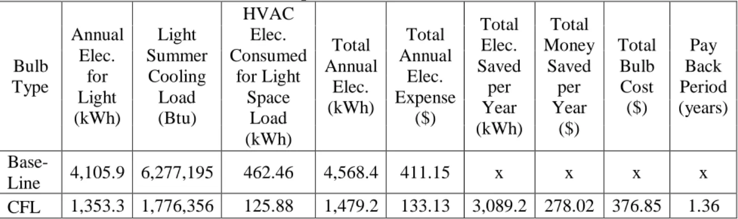
Two companies have brought (or are about to bring) competitive LED lighting technologies into the market place. The Philips EnduraLED™ uses only 12 Watts of power to produce 806 lumens of light. This corresponds to the light production of a typical 60 Watt incandescent bulb but with an efficacy of nearly 67.17 lm/W. These lights are rated to last 25,000 hours but are much more expensive than tradition bulbs. Phillips estimates each bulb will cost about $50.00, and expects them to be commercially available by the end of 2010 (early 2011). Likewise, The Home Depot® has produced its own brand of LED light called the EcoSmart™ LED A19. This bulb uses 8.6 Watts of power to produce 429 lumens of light (comparable to a 40 Watt incandescent bulb). This corresponds to an efficacy of 49.88 lm/W. Despite having less light output (lumens) than a standard 60 Watt incandescent bulb, the EcoSmart™ boasts a 50,000 hour life rating and will only cost $17.97 per bulb at Home Depot stores worldwide.

A comparison of some of the lighting options (Incandescents, Fluorescents, and LEDs) commercially available at local, home improvement stores are shown in Tables 3.1, Table 3.2, and Table 3.3. These tables list the power consumption (wattage), light production (lumens), efficacy (lm/W), life-time rating (hours of operation), and cost of each bulb for various light options that will be important later in this chapter. All of these values (except for the calculated efficacy numbers) were taken directly off the packaging information for each light bulb option.

Table 3.1: Incandescent Light Bulbs Commercially Available

Incandescent Lights Power (W) Light Output (lm) Efficacy (lm/W) Life (hrs) Price ($/bulb)

GE 40 Decorative Pointed Display Bulb 40 455 11.38 1,500 1.37 Sylvania Soft White 60 Standard Bulb 60 850 14.17 1,500 1.91 Sylvania Soft White Double Life 75 75 1085 14.47 1,500 1.91 Sylvania Soft White Double Life 100 100 1590 15.90 1,500 1.91 Sylvania Soft White Double Life 150 150 2740 18.27 750 3.14 Sylvania 15172 BR30 Indoor Flood Light 65 580 8.92 2,000 4.15 Energy Wise 50 Narrow Indoor Flood 50 660 13.20 2,500 6.95 SLI Lighting 150 Outdoor Flood Light 150 1730 11.53 5,000 2.80

GE Halogen Outdoor Flood 90 1310 14.56 6,000 9.87

Table 3.2: Fluorescent Light Bulbs Commercially Available

Fluorescent Lights Power (W) Light Output (lm) Efficacy (lm/W) Life (hrs) Price ($/bulb)

Linear Fluorescent 40W T12 Commercial 40 2000 50.00 20,000 1.30 EcoSmart 7 Decorative Bulb Regular CFL 7 350 50.00 8,000 3.32

EcoSmart 9 Regular CFL 9 470 52.22 8,000 4.99

Bright Effect 11 Regular CFL 11 400 36.36 6,000 4.88 Sylvania Micro-mini 13 Regular CFL 13 820 63.08 12,000 3.49 Bright Effects 13 Regular CFL 13 825 63.46 8,000 2.49 Lumacoil Energy Saving Regular CFL 13 900 69.23 12,000 1.65

EcoSmart 14 Regular CFL 14 465 33.21 8,000 4.99

Phillips Energy Saver 16 Regular CFL 16 630 39.38 8,000 11.98 AM Conservation Group AM20PERM CFL 20 1200 60.00 10,000 2.53 Bright Effects 20 Regular CFL 20 1250 62.50 10,000 2.03 Phillips Marathon Regular CFL 20 930 46.50 8,000 11.99 Sylvania Micro-mini 23 Regular CFL 23 1640 71.30 12,000 3.99 EcoSmart 14 Indoor Flood CFL 14 640 45.71 8,000 4.49 GE Energy Smart Indoor Flood CFL 15 750 50.00 10,000 4.88 GE Energy Smart Indoor Flood CFL 15 720 48.00 6,000 11.00 GE Energy Smart Indoor Flood CFL 23 1185 51.52 10,000 7.16 EcoSmart 23 Indoor Flood CFL 23 1100 47.83 8,000 7.97 GE Energy Smart Outdoor Flood CFL 23 1185 51.52 10,000 8.13 Bright Effects Outdoor Flood CFL 26 1300 50.00 8,000 6.68

Table 3.3: LED Lights Commercially Available

LED Lights Power

(W) Light Output (lm) Efficacy (lm/W) Life (hrs) Price ($/bulb)

Phillips Deco 2.5 Regular LED 2.5 30 12.00 15,000 7.99

Phillips 5 Regular LED 5 240 48.00 25,000 24.97

Feit Electric Regular LED 6.5 340 52.31 30,000 18.98 Sylvania Ultra 8 Dimmable LED 8 430 53.75 50,000 19.98

Phillips 8 Regular LED 8 450 56.25 25,000 21.97

EcoSmart 8 Regular LED 8 450 56.25 50,000 29.97

Home Depot EcoSmart LED A19 8.6 429 49.88 50,000 17.97 Philips EnduraLED 60W Replacement 12 806 67.17 25,000 50.00 Phillips 12.5 Regular LED 12.5 800 64.00 25,000 39.97 Phillips 7 Indoor Flood LED 7 155 22.14 40,000 29.97 Feit Electric 8 Indoor Flood LED 8 350 43.75 30,000 24.97 EcoSmart 8 Indoor Flood LED 8 350 43.75 50,000 24.97 Phillips 11 Indoor Flood LED 11 430 39.09 25,000 49.97 EcoSmart 15 Indoor Flood LED 15 725 48.33 50,000 39.97 Feit Electric 16 Indoor Flood LED 16 728 45.50 30,000 59.98 Phillips 16 Indoor Flood LED 16 600 37.50 25,000 69.97 Sylvania Ultra 18 Indoor Flood LED 18 900 50.00 50,000 44.98 EcoSmart 18 Indoor Flood LED 18 850 47.22 50,000 44.97 Phillips 16 Outdoor Flood LED 16 850 53.13 20,000 64.97