UC Davis
IDAV Publications
Title
Time and Streak Surfaces for Flow Visualization in Large Time-Varying Data Sets
Permalink
https://escholarship.org/uc/item/35j0j63w
Authors
Krishnan, Hari
Garth, Christoph
Joy, Ken
Publication Date
2009
Peer reviewed
eScholarship.org
Powered by the California Digital Library
Time and Streak Surfaces for Flow Visualization
in Large Time-Varying Data Sets
Hari Krishnan, Christoph Garth, and Kenneth I. Joy,Member, IEEE
Abstract—Time and streak surfaces are ideal tools to illustrate time-varying vector fields since they directly appeal to the intuition about coherently moving particles. However, efficient generation of high-quality time and streak surfaces for complex, large and time-varying vector field data has been elusive due to the computational effort involved. In this work, we propose a novel algorithm for computing such surfaces. Our approach is based on a decoupling of surface advection and surface adaptation and yields im-proved efficiency over other surface tracking methods, and allows us to leverage inherent parallelization opportunities in the surface advection, resulting in more rapid parallel computation. Moreover, we obtain as a result of our algorithm the entire evolution of a time or streak surface in a compact representation, allowing for interactive, high-quality rendering, visualization and exploration of the evolving surface. Finally, we discuss a number of ways to improve surface depiction through advanced rendering and texturing, while preserving interactivity, and provide a number of examples for real-world datasets and analyze the behavior of our algorithm on them. Index Terms—3D vector field visualization, flow visualization, time-varying, time and streak surfaces, surface extraction.
1 INTRODUCTION
Integral curves have a long standing tradition in vector field visualiza-tion as a powerful tool for providing insight into complex vector fields. They are built on the intuition of moving particles and the representa-tion of their trajectories. A number of different variants exist; while streamlines and pathlines directly depict single particle trajectories, other curves visualize the evolution of particles that are seeded co-herently in space (time lines) or time (streak lines). These curves have their roots in experimental flow visualization and correspond to smoke or dye released into a flow field. Generalizing on these concepts, inte-gral surfaces extend the depiction by one additional dimension.
Stream and path surfaces aim to show the evolution of a line of particles, seeded simultaneously, over its entire lifetime. These sur-faces have been shown to provide great illustrative capabilities and much improved visualization over simple integral curves, due to im-proved depth perception and lighting, and increase the visual insight into flow structures encountered during their evolution. Time surfaces increase the dimensionality further by showing the evolution of a two-dimensional sheet of particles. Finally, streak surfaces borrow from both path surface and time surfaces by portraying an evolving sheet of particles that grows during the evolution at a seeding curve as new particles are added to the surface. They are analogous to streak lines in that they originate from wind tunnel experiments with line-shaped nozzles, and are therefore in a sense a very natural surface visualiza-tion primitive for time-varying flows.
Application of integral surface visualization to large, complex and time-varying flow is not without complication. Typical algorithms for the approximation of stream and path surfaces make use of a form of discretization to deduce the evolution of the surface from a finite set of particles representing it. The required integral curve computation is costly for large vector fields, and most algorithms make use of adap-tive techniques to keep the number of required particles small, while preserving the geometric quality of the resulting surface discretiza-tion. Such methods typically require pre-computation of the integral surface, which can then be viewed interactively as a triangle mesh. Un-fortunately, such methods do not generalize well to time or streak sur-faces because they cannot provide interaction with the temporal
com-• Hari Krishnan, Christoph Garth and Ken Joy are with the Institute of Data Analysis and Visualization, University of California, Davis, E-mail: {hkrishnan|cgarth|kijoy}@ucdavis.edu.
Manuscript received 31 March 2009; accepted 27 July 2009; posted online 11 October 2009; mailed on 5 October 2009.
For information on obtaining reprints of this article, please send email to: [email protected] .
ponent of the surface evolution. For small to medium-sized rectilinear datasets, GPU-based implementations have shown the tremendous po-tential for insight that can be obtained from interaction with time in time and streak surface visualization.
Here, we contribute a novel method for the computation of time and streak surfaces that captures the temporal evolution of such surfaces for visualization. Our algorithm is based on decoupling the adaptation of the surface representation from the integration of particle ries. As a result, we obtain a set of curves that describe the trajecto-ries of surface vertices, and an incremental description of the surface mesh based on these particles trajectories. This allows us to faithfully recreate a surface in a visualization stage and provide full interactive capabilities in both space and time. Furthermore, by isolating particle advection from surface adaptation, we are able to leverage the full par-allelization potential inherent in the mutually independent trajectories of individual surface particles and significantly speed up the compu-tation in the presence of multiple CPUs or clusters. Moreover, not-ing that for very large datasets interactive seednot-ing of time and streak surfaces remains elusive due to the computational overhead of their approximation, we propose the concept ofgeneralizedstreak surfaces seeded from a moving seed curve. We show that through this, we are able to mitigate some of the difficulties of surface seeding in large vector fields by essentially prescribing an exploratory path for the seed curve prior to computation.
The surfaces we obtain in complex datasets are often highly com-plex, due to their folding and twisting nature, and warrant the use of advanced rendering techniques to increase the visual insight resulting from them. Here, we investigate a number of typical complications, such as self-occlusion, and analyze possibilities on how to mitigate them to achieve maximal visualization value from time and streak sur-faces.
The paper is structured as follows: We start out by discussing pre-vious work that related to the ideas presented here in Section 2. After revisiting the basic surface concepts we make use of in Section 3, we describe our algorithm for the computation of time and streak surfaces in Section 4. We then proceed to describe application examples and investigate the behavior and performance of our method in Section 7. Following, we examine visualization aspects of time and streak sur-faces in Section 6, before we conclude on the presented material in Section 8 and look ahead to future work.
2 PREVIOUSWORK
Among integral surfaces, stream surfaces have been most heavily in-vestigated in the visualization community. The first algorithm for stream surface computation was given by Hultquist [7], who described
an advancing front paradigm that traverses the surface, integrating par-ticle trajectories as needed and triangulating the surface on-the-fly us-ing a greedy approach. In his algorithm, divergence and convergence of particles in the advancing front is treated using a distance crite-rion that inserts and removes particles from the advancing front if they grow too far apart or too close, respectively. The resulting surfaces are of good visual quality. Garth et al. [5] improved upon Hultquist’s work by employing arc-length particle integration and additional curvature-based front refinement, which results in a better surface triangulation if the surface strongly shears, twists, or folds. They also considered vi-sualization options such as color mapping of vector field-related vari-ables going beyond straightforward surface rendering. Texture map-ping on stream surfaces was first proposed by L¨offelmann [10], and several improvements were presented later [9]. A different compu-tational strategy was employed by van Wijk [15], who reformulated stream surfaces as isosurfaces; however, his method requires increased computational effort to advect a boundary-defined scalar field through-out the flow domain. Scheuermann et al. [13] presented a method for tetrahedral meshes that solves the surface integration exactly per tetra-hedron. More recently, Garth et al. [4] replaced the advancing front paradigm by an incremental time line approximation scheme, allow-ing them to keep particle integration localized in time. They applied this algorithm to compute stream surfaces and path surfaces in large and time-varying datasets. Using a GPU-based approach, Schafhitzel et al. [12] presented a point-based algorithm that does not compute an explicit mesh representation but rather uses a very dense set of parti-cles, advected at interactive speeds, in combination with point-based rendering.
The increased complexity of time and streak surface computation over stream and path surfaces can be traced back to two main factors: first, many more particles are required for adequate discretization, and second, instead of an advancing (piecewise linear) front or time line a surface discretization has to be maintained and adapted. In the litera-ture, the first problem is usually addressed by GPU implementations, allowing for fast or even interactive computation of the required parti-cles. Westermann et al. [17] approached the visualization of time sur-faces in stationary flow using a level-set approach, where the surface is described as the level set of a scalar field that is advected at inter-active speeds on a GPU. This allows for interinter-active computation and display, and avoids the explicit surface adaptation. A slightly different approach was presented recently by Funck et al. [16]: they represent time and streak surfaces using a triangle mesh which is propagated along the trajectories of particles at the vertices of the triangulation, integrated on the CPU. Instead of performing surface adaptation, the mesh remains unchanged, and loss of mesh quality is compensated by fading out triangles according to a number of quality criteria, mimick-ing the appearance of smoke. While they achieve aesthetically pleas-ing visualization in combination with interactive framerates and seed-ing, the resulting surfaces are of limited use in complex flows where the initial triangulation quickly degenerates. All methods that make use of GPUs to compute time and streak surfaces possess the common drawback that they are unsuitable for very-large time-varying data, due to the limitation to regularly sampled data, the reduced amount of memory available on GPUs, and the restriction to floating-point precision during the integration phase. In contrast to these approaches for time and streak surfaces, the algorithm we present here is explic-itly aimed at a CPU-based treatment of very large, time-varying vector fields. We maintain an explicit triangulation for the surface and adapt it as the surface is advected through the flow. To increase compu-tational speed, however, we separate this mesh adaptation from the actual particle integration, allowing us to parallelize particle tracing.
The dynamic adaptation of deforming and moving triangle meshes has a long record in the computer graphics community where it is ap-plied among other applications to track and render fluid surfaces and to simulate cloth and elastic objects (cf. [2] and references contained therein). The basic objective of such surface tracking methods is to maintain a well-conditioned triangulation in the face of strong defor-mations of the surface, by using edge split, edge flip and edge collapse operations to return a mesh to good form after an advection step has
been performed. While such tracking algorithms are theoretically a good match to the adaptation of time surfaces, a straightforward appli-cation encounters several problems that stem from the simulated and numerical nature of the datasets under consideration such as noise and limited accuracy of interpolation. Furthermore, these methods require to advect the mesh by very small time steps, such that the deformation incurred during advection is not too great; this represents a serious performance impediment for large datasets, where the use of adaptive numerical integration for particle advection is essential to both per-formance and accuracy. Here, we propose a modified approach that decouples the surface adaptation from the particle advection, thereby avoiding the performance penalty of small adaptation time steps.
3 TIME ANDSTREAKSURFACES
We assume thatvis a three-dimensional vector field, defined over a domainΩ⊂R3and a time interval[Tmin,Tmax]. Anintegral curve Iof
vis the solution to the ordinary differential equation
d dtI(t0,x0)(t) t= τ =v τ,I(t0,x0)(τ) , withI(t0,x0)(t0) =x0. (1)
Simply put, it is a curve that originates at the point(t0,x0)and is
tangent to the vector field at every point over time. The intuitive under-standing associated with such integral curves is that of massless par-ticles that are advected through a domain by a vector fieldv. For the category of Lipschitz-continuous vector fields existence and unique-ness ofIis guaranteed and numerical integration methods can be used to approximate the solution. Note that for the overwhelming majority of application data sets, this condition holds true.
Atime surface Stimeis a two-dimensional family of integral curves that originate from a common seed surface S(u,v)⊂Ω, or
alterna-tively, the surface formed by a dense set of particles that are located onSat timet0and jointly traverse the flow over a time interval[t0,t].
It is mathematically described as
Stime(u,v;t):=I(t0,S(u,v))(t) fort≥t0. (2)
Furthermore, letC(u)be a curve, parameterized overuand con-tained inΩ. Then, astreak surface Sstreakis the union of all particles emanating continuously fromCover a time interval[t0,t]and moving
with the flow from the time of their seedingts. In terms of individual
integral curves, it is described as
Sstreak(u,ts;t):=I(ts,C(u))(t) fort≥ts≥t0. (3)
It is again a two-dimensional surface, but in contrast to time sur-faces, the second parameterts refers to the seeding time. Clearly, a
streak surface consists only of the curveCat timet0and “grows” over
time as more integral curves are seeded fromC; the intuition behind streak surfaces builds upon the notion of dye continuously injected into a flow from a curve-shaped nozzle, described byC. Following Wiebel et al. [18], we extend the above definition of streak surfaces slightly to allowCto vary with time. The above definition is then gen-eralized by replacingC(u)withC(u;ts), and the resulting surfaces are
calledgeneralized streak surfaces.
Note that if the vector field is stationary, i.e. vis constant int, then the path of particle does not depend on the seeding timet0. As
a consequence, streak surfaces are identical to path surfaces (cf. [4]) in such settings. However, this does not hold for generalized streak surfaces. Both surface types are continuous and differentiable almost everywhere over their respecitve parameter domains. However, as is often the case in application vector field data, ifΩis finite or contains holes, the resulting surfaces may not include points for all parameters tuples(u,v;t)and(u,ts;t), respectively.
We proceed to describe an algorithm to construct approximations to bothStimeandSstreakusing a finite number of integral curves and triangulated surface adaptation.
(a) Edge split (b) Edge flip (c) Edge collapse Fig. 1. Three types of surface mesh operations used to adapt the surface resolution during advection.
4 METHOD
In the following, we first give an overview about our algorithm in gen-eral, before we detail integration, adaption, and surface growing.
4.1 Basic Algorithm
In general, we assume that the vector field dataset under consideration is provided in the form of a finite number of time steps correspond-ing to time valuest0, . . . ,tn, and that the seeding curveCor surfaceS
is provided in the form of either a functional description or as a dis-crete representation as polyline or triangulated surface. From this, we construct an initial triangulationT that is successively advected and adapted. Our algorithm thereby makes use of two distinct time step-ping approaches.
Every vertex ofT corresponds to an integral curve, and we advect vertices over an interval[ti, . . . ,ti+1]using adaptive numerical
integra-tion, obtaining a description of the integral curves over the entire in-terval (cf. 4.2). In contrast to thisdataset timestep∆t, we prescribe an
adaptation timestep∆tsub. Beginning atti, the vertices ofTare moved
in∆tsubincrements, and after every step, the adaptation process is
car-ried out. Should the insertion of a new vertex become necessary, the seed point of the corresponding integral point is determined atti, and
the curve is numerically propagated over[ti,ti+1]; this serves to
min-imize the error during the insertion. If the vertices arrive atti+1, the
process is restarted, withT as the new initial surface. Figure 2 pro-vides an overview of this algorithm is pseudocode form.
We observe two basic properties of the above algorithm:
• Most integral curve computations are performed at the beginning of a new time interval[ti,ti+1]. Hence, these mutually
indepen-dent computations are trivially parallel and can be carried out in a distributed fashion using multiple CPUs or cluster nodes.
• The surface approximation is sequential in time, and thus succes-sive pairs of timesteps can be treated in a streaming fashion. This enables the treatment of very large datasets on smaller hardware, subject only to the constraints that two timesteps fit into main memory simultaneously.
We will first describe the numerical implementation we use to approx-imate integral curves.
4.2 Integral Curve Computation
In large vector fields with complex structures, high-order adaptive nu-merical integration is the key to efficient approximation of integral curves. In our surface approximation, we make use of the DOPRI5 scheme, an adaptive Runge-Kutta scheme of fifth order [6, 11]. This scheme was first used for visualization purposes by Stalling [14], and its appeal for our application is founded on its ability to provide dense output, i.e. to represent the numerically approximated particle tra-jectory as a sequence of fourth-order polynomials that form aC 1-continuous curve. From this curve, any point in the interim evolution of the integral curve is readily computed, and the numerical scheme can perform its task with optimal adaptive stepsize control and is un-constrained by a limit on the maximal distance between two consec-utive points on the integral curve (as is the case with other adaptive schemes).
After the integral for all vertices ofT have been computed over
[ti,ti+1],Tis advanced towardsti+1using the much smaller step∆tsub.
The new vertex positions are interpolated from the piecewise polyno-mial representations of the corresponding integral curves. We next de-scribe the surface adaptation that is applied after every such advance-ment.
4.3 Surface Adaptation
During the adaptation phase, the three basic operations edge split, edge flip, and edge collapse (see Figure 1) are applied to the triangulation
Tto improve the quality of the tracked surface. We next describe each of these in more detail.
4.3.1 Edge Split
Since the approximation quality of a triangle mesh is, among other factors, a function of the maximal edge length, we split all triangle edges that are longer than a prescribed thresholddmax. Here, a new
vertex is inserted at the center of the edge together with a new integral curve seeded at the center of the edge corresponding to the beginning of the dataset timestep,ti. The integral curve is then propagated toti+1,
and the position of the inserted vertex determined from the integral curve at the current adaptation time. The resulting mesh depends on the order of splits, and we split the longest edge first to keep the mesh well conditioned (refer also to Jiao et al. [8]). Splits of boundary edges require no special treatment and are performed analogously to interior edges.
Two exceptional situations can occur during a split operation. First, the new integral curve may not reach the current adaptation time be-cause it intersected a boundary or numerical integration failed. Sec-ond, the modified triangulation can contain triangles with inverted nor-mals, since an inserted vertex moved outside the area covered by the original triangles neighboring the edge. In both cases, we insert the vertex at the geometric midpoint of the edge at the current time, and
advance_surface( T, t_start, t_end ) {
t_stop = load_first_timestep( t_start ); t_current = t_start;
do {
integrate_curves( T, t_stop );
do {
delta_t = estimate_timestep();
t_current = min( t_current + delta_t, t_stop );
update_vertices( T, t_current ); add_streak_part( T, t_current );
split_pass( T ); flip_pass( T ); }
while( t_current < t_stop );
collapse_pass( T );
t_stop = min( t_end, load_next_timestep( t_current ) ); }
while( t_stop > t_current );
}
(a) Inverted triangles (b) Degenerate triangles (c) Volume change Fig. 3. Degenerate cases to be avoided when flipping an edge.
seed a new integral curve from this point at the current time. If, again, the current point is not contained within the flow domain, we consider the insertion attempt as failed and remove the edge-adjacent triangles from the triangulation. While we could simply keep these triangles in place and not perform the split, we have found this to quickly produce degenerate triangulations. Furthermore, the accuracy of the surface in such a region is questionable, since the necessary refinement could not take place.
To make the adaptation more robust with respect to erratic numer-ical integration that is often encountered in simulation datasets (cf. Section 7), we place a very small lower boundAmin on the area of
triangles that result from the edge split and do not carry it out if this bound is not fulfilled to prevent infinite refinement.
In addition to linear edge midpoint insertion, there are other schemes to determine the placement of newly inserted edge midpoints, such as the quadratic error minimizing insertion scheme [3] and the general subdivision schemes such as Butterfly- or√3-subdivision. We have found however that these methods do not perform very well in our algorithm since they tend to emphasize small scale oscillations, which then quickly lead to large approximation errors.
4.3.2 Edge Flip
Edge flipping is commonly used in meshing algorithms such as e.g. Delaunay triangulation. Here, it serves the purpose of improving the local quality of the mesh by maximizing the minimum angle, increas-ing the approximation quality of the surface triangulation and makincreas-ing it geometrically more well-conditioned. An edge is considered flip-pableif its potential length after a flip decreases by at least a fixed ratio, which we generally chose as 0.9 to balance excessive flipping with mesh improvement. Again, to avoid degeneracies such as very small or inverted triangles (cf. Figure 3), we compute the triangle area and normals of the edge-adjacent triangles, and do not proceed with the flip operation if the normals are inverted or the resulting triangles do not surpass the small area bound. To prevent flipping of edges that are located on relatively sharp ridges of the surface, we compute the volume of the tetrahedron spanned by the edge vertices and the two opposing vertices; this models the local change of volume enclosed by the surface incurred by flipping. If this volume exceeds a thresh-oldVmax, the edge is consideredunflippable. We have observed this
additional criterion to markedly increase the representation of ridges where the surface folds strongly. While other criteria such as e.g. the dihedral angle can be used to identify such creases, we prefer volume change as a more robust criterion since it is scale-dependent and avoids over-refinement in the presence of small-scale noise.
Applying the above criteria, we traverse all edges of the triangula-tion (except the boundary edges) and flip any edge that is considered flippable. As in some regions, several flip operations can be required to achieve optimal quality, we repeat this flipping traversal a small number of times.
4.3.3 Edge Collapse
In the case of strong convergence of integral curves, the triangulation will come to contain very small triangles, and the number of vertices in such regions becomes excessive. To improve the surface triangulation and reduce the number of integral curves to be propagated in further time steps, we perform edge collapse operations. As opposed to splits and flips, we perform this operation only at the end of the current data timestepti+1such that we do not lose approximation accuracy when it
is required to perform a split and consequently insertion atti.
We consider edges whose length is below a prescribed minimum edge lengthdminas eligible for collapse. For each such edge, we
de-termine the vertex to be deleted from the triangulation by determining the volume change incurred by the removal of either vertex, and re-moving the vertex that represents the smaller volume change. This pe-nalizes the removal of edges that are located along ridge-like regions of the surface and improves the approximation of strongly folding sur-faces. If the volume change exceedsVmax, the collapse is aborted. In
similarity to the split operation, we collapse eligible edges in order of ascending edge length. We have again found that replacing an edge by a new midpoint as chosen from quadratic error minimization or sub-division does not yield good results, especially in regions where the surface is ridge-shaped or otherwise non-smooth.
4.3.4 Parameters
The adaptation phase detailed above makes use of a variety of param-eters that have to be carefully chosen to balance triangle mesh refine-ment, coarsening, and approximation quality. We reduce the number of parameters that have to be chosen by coupling them todmax, using
dmin=0.1dmax,Amin=0.1dmin2 , andVmax=d 3
min. We have applied
this heuristic in all of our experiments and have observed the result-ing surfaces to be of good quality, as demonstrated in Figure 4 and Section 7. Hence, the remaining parameterdmaxtakes the form of a
scaling parameter that must be chosen to roughly reflect the scale of the smallest structures that the surface must resolve correctly.
4.3.5 Step Size Estimation
In order to guarantee that the surface can be adapted correctly, the adaptation timestep∆tsubmust be chosen such that the triangulation
does not undergo irreparable changes in between adaptations. Typi-cally, such a timestep is chosen much smaller than the dataset timestep
∆t. To avoid burdening the user with the choice of this timestep, we select it automatically by requiring that no vertex of the triangulation moves further thandmaxfrom its current position. As a consequence,
no edge can grow to more than twicedmaxin length, and has to be split
no more than once per adaptation step.
Using the piecewise polynomial integral curve representation de-scribed above, this criterion is easily approximated by evaluating the current speed of any vertex in the triangulation by evaluating the derivative magnitude of the integral curves through interpolation. This avoids the overhead of additional costly vector field evaluations at ev-ery vertex position. Then, if the maximal determined vertex velocity is denoted byvmax, we select the next adaptation time step as
∆tsub:=dmax/vmax.
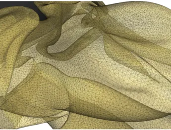
Fig. 4. Time surface mesh in the Ellipsoid dataset. Although the surface has undergone strong deformation, the mesh remains in good condition.
4.4 Streak Surface Growing
So far, we have discussed an algorithm that is able to propagate and adapt a time surface as it is advected by a given vector field. To ap-ply the same algorithm to streak surfaces and generalized streak sur-faces, the surface must be extended to reflect the new particles seeded continuously at the (moving) seeding curve. To guarantee adequate discretization of this small part of the surface, we apply the following scheme.
At the initial time, a number of vertices and edges connecting them into a polyline are placed on the seeding curveCsuch that they fulfill the maximum edge length criterion. Then, the vertex positions and the seeding curveCare advanced in time, and the resolution is maintained using edge splitting. If any surface vertex moves more thandmaxaway
from the seeding curve, two triangles connecting the surface edge to the seeding curve are generated by placing two new vertices on the seeding curveC. This straightforward scheme works well even in the presence of a rapidly moving seeding curve.
4.5 Output
After a time or streak surface has been approximated, the evolution of the surface can be completely recreated from the initial mesh using the following observations:
• The position of any vertex with respect to time can be interpo-lated from the piecewise representation of its corresponding in-tegral curve.
• The evolution of the topology of the triangle mesh describing the surface can be recreated at any given point in time by sequen-tially applying all edge operations (splits, flips, and collapses) that were applied during surface adaptation up to the desired time.
Consequently, we record the topological changes to the mesh together with the time at which they were performed in a list. Both the list and all integral curve representations are saved during and after the surface computation. With this representation, we do not require to store a triangle mesh for every step at which the surface changes; this would be prohibitively expensive as the number of changes to the mesh can be very large for complex surfaces. Hence we obtain a very compact representation of the full surface evolution which serves as input to our surface visualization, as described in the Section 6.
5 PRACTICALCONSIDERATIONS
We now detail some aspects of the behavior of our algorithm when applied to extract integral surfaces from large, complex simulation datasets.
5.1 Numerical Aspects
In general, there are two sources of error in the surface approxima-tion: first, approximation error is incurred by the discrete nature of the surface. Here, the approximation accuracy crucially depends on the maximal length of the surface mesh edges, as well as on the shape of the triangles, where skinny triangles must be avoided to achieve good approximation. A secondary source of error is the insertion of new vertices into the surface triangulation. Since edge midpoints do not exactly represent the curvature of the surface, the inserted vertex is not exactly located on the surface, and in a worst case scenario, small er-rors introduced by this may be exponentially magnified by the integral nature of the surface. However, both errors tend to zero as the max-imum edge length is decreased. This fact is leveraged by the longest edge bisection criterion, as is customary in surface refinement. To in-vestigate the correctness and accuracy of our adaptive algorithm, we have compared select surfaces against non-adaptive, high-resolution surfaces propagated from the same seed surface or curve and verified that the error is reduced with decreasing maximum edge length.
A different source of errors stems from the use of numerical inte-gration. In significantly complex simulation data, such interpolation can be unreliable; this problem is encountered especially in the close
vicinity of domain boundaries. As described above, we have added a number of criteria to our algorithm to make it more robust in the face of such difficulties. In the worst cases, instead of continuing with a possibly incorrect surface, we opt to rather remove the corresponding vertices or edges from the triangulation. Fortunately, such missing tri-angles are relatively rare and do not have a significant impact on the resulting surface visualizations.
5.2 Performance
The performance of our algorithm depends strongly on the number of vertices in the surface triangulation and, correspondingly, on the number of integral curves that must be computed for any given sur-face. Performing such computations in highly resolved complex data is an expensive task. Especially the unstructured datasets consisting of mixed element types that we have used to evaluate our method (Sec-tion 7) requires careful cell loca(Sec-tion and interpola(Sec-tion. This is reflected in substantial running times of our algorithm. While significantly bet-ter performance could be easily achieved for rectilinear datasets, such as those produced by DNS simulations, our goal is to document the performance of our algorithm on the finite-element meshes that are ubiquitous in CFD practice.
Table 1 provides the performance figures corresponding to the sur-faces shown in Figures 4-9. We observe that in all cases, more than 90% of computation time is spent in integration. However, this com-putational effort is rewarded with a surface that accurately reflects the vector field under consideration. Furthermore, we maximize the vi-sualization result by not only providing a final surface, but also mak-ing accessible to visualization the entire surface evolution in compact form. Finally, the ability of our algorithm to compute generalized streak surfaces alleviates the problem of iterative seeding refinement. By letting a streak surface seed curve traverse a region of interest, an entire volume of flow can be investigated in one computational pass. Furthermore, the observed scaling factors on an 8-way SMP system in-dicates that we have managed to leverage the inherently parallel nature of massive integral curve computation in the parallel implementation of our algorithm.
6 VISUALIZATION
The computation times incurred by our algorithm are significant if complex surfaces are to be accurately approximated. Presenting the user with a final mesh is unsuitable, since the ability to depict the evo-lution of the surface is crucial to comprehend the behavior of the flow it depicts. Providing the ability to navigate freely in time when visu-alizing the surface is helpful in understanding how certain parts of a surface evolve. Our approximation algorithm is ideally suited to this purpose since we can trivially and efficiently recreate the surface at any given point during its advection.
High-quality rendering is a crucial aspect of graphically depicting highly complex time and streak surfaces. This has recently been doc-umented independently by Garth et al. [4] and von Funck et al. [16]. Correct surface lighting and shading provide important depth cues to the viewer, and we have found that multiple light sources can further enhance the spatial perception of the surfaces we visualize. Since the surfaces we compute and visualize are often self-occluding, correct
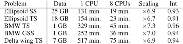
Problem Data 1 CPU 8 CPUs Scaling Int Ellipsoid SS 25 GB 131 min. 19 min. ×6.9 0.93 Ellipsoid TS 18 GB 154 min. 23 min. ×6.7 0.91 BMW TS 1 GB 329 min. 45 min. ×7.3 0.96 BMW GSS 1 GB 252 min. 36 min. ×7.0 0.94 Delta wing TS 7 GB 517 min. 75 min. ×6.9 0.94
Table 1. Performance measurements for the five test problems de-scribed in Section 7 (TS = time surface, (G)SS = (generalized) streak surface). All measurements were performed on a quad-core AMD Opteron 2.4GHz with 8GB RAM. “Data” refers to the amout of data streamed during the computation. “Int” denotes the fraction of com-putation time spent on integral curve comcom-putation.
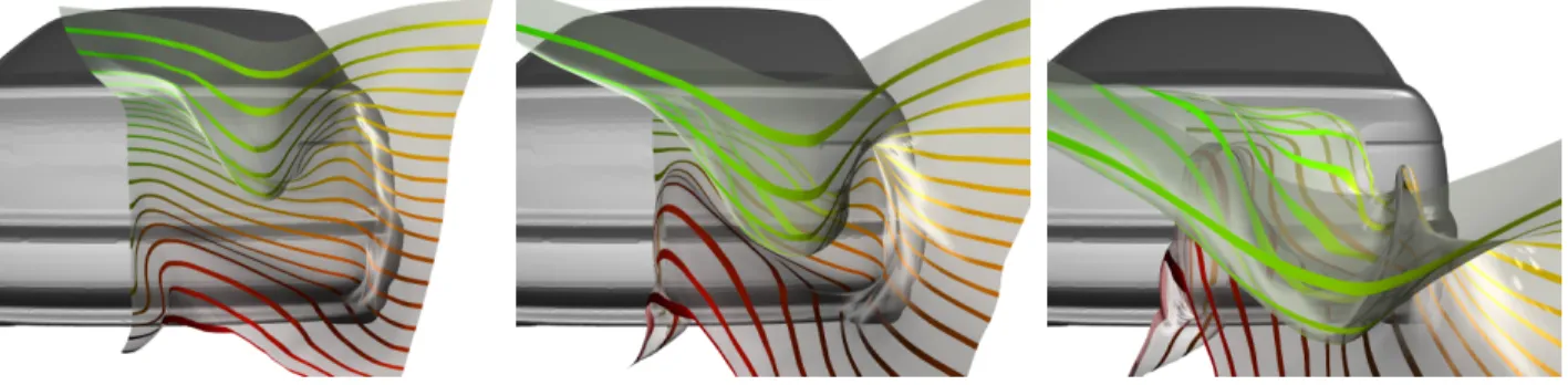
Fig. 5. Three frames from an animation showing the evolution of a time surface in the BMW dataset. The surfaces is seeded on a square at the rear end of the car and illustrates the recirculation of air in this region of the flow. A streak ribbon texture provides additional depth cues.
handling of transparency is important. Furthermore, texturing of the surface can further help to orient a viewer looking at such a surface. As is apparent from Equations 2 and 3 above, both types of surfaces offer natural texture coordinates from their two-dimensional parameteriza-tion. While for time surfaces the parameters do not possess special meaning, streak surfaces allow texture mapping to depict both time lines (lines of constantt0) and streak ribbons (lines of constantu), as
depicted in Figure 7. We make use of these mappings to depict the surfaces using stripes of relatively high opacity interleaved by areas of low opacity that provide surface context. In cases where the stripes do not work well, such as when many surface layers are nested very closely, we still apply a simple two-dimensional color map to the sur-face; this helps in distinguishing different surface parts visually (see e.g. Figure 8).
To allow for interactive visualization under these constraints, we have implemented a visualization tool that incorporates all the dis-cussed options. Good performance in the presence of transparency and high depth complexity is achieved by using the dual depth peeling technique described by Bavoli and Myers [1], and high-quality light-ing and texture mapplight-ing is achieved through the use of pixel shaders. Reconstructing the surface at a given point in time is performed on the CPU; our implementation is fast enough to handle quick and interac-tive temporal navigation even for large surfaces. The surfaces shown in Figures 4–9 are rendered and animated at interactive speeds of 20– 60 fps on commodity hardware.
7 EXAMPLES
To demonstrate our method, we have applied it to compute various surfaces in three different application datasets. Here we show the re-sulting surfaces as rendered by our visualization tool.
Ellipsoid The Ellipsoid dataset results from an unsteady
simula-tion of the flow around an ellipsoid, where the angle of the surrounding flow changes over time. Vortex formation near the downstream bound-ary of the embedded ellipsoid can be observed. The data consists of am unstructured mesh of 2.6 million hexahedral cells, over which the flow field is given in 600 time steps. This dataset is very well resolved and represents a relatively well behaved and smooth case with very good temporal resolution.
Figure 7 depicts a single streak surface seeded and computed over ca. 70% of the temporal extent of the dataset. Seeding was initialized at the initial timestep on the upstream side of the ellipsoid, and the streak surface nicely captures the transitionary stage during the vortex formation that forms a bubble shaped structure. In the upper image of Figure 7, time line texturing has been applied, and it is straightfor-ward to distinguish parts of the surface that were seeded later (greener stripes) from those that were seeded earlier (redder stripes), allowing good temporal orientation. In the lower left image, streak line textur-ing has been applied to illustrate the paths of different streaks. Again, a variation in the color of the stripes provides both spatial and tempo-ral context. For comparison, the lower right image does not make use of texturing; there, no correlation between surface points and seeding time or origin can be made. To integrate the surface, 30,028 integral
curves were traced and 268,171 mesh adaptation operations were per-formed.
A time surface in the same dataset seeded on a rectangle just down-stream of the ellipsoid in the initial timestep and traced over ca. 50% of the dataset extent in time is shown in Figure 8. The surface con-sists of 102,764 pathlines and required 691,916 adaptation operations. In this figure, we have opted for a simple two-dimensional color map since there is no natural texturing for time surfaces. During the evolu-tion of the surface, it wraps around the nascent, forming vortex system, and encounters strong deformation when it is laterally drawn into the forming vortices. The resulting final surface mesh is illustrated in Fig-ure 4. Both surfaces demonstrate the ability of our algorithm to deal with data set sizes strongly exceeding available main memory.
Car This steady simulation models the flow of air around a car. Vortex shedding can be observed on various parts of the car. The flow vector field is represented on an unstructured mesh with 15 million elements of mixed type. Since the flow is assumed symmetric with re-spect to the symmetry axis of the car, the computational domain con-tains only the right side of the car. Figure 5 illustrates a time surface seeded just downstream of the rear end. The upper part of the surface moves away from the car quickly, but the lower part is drawn into a large vortex emanating from the edge of the rear bumper. A striped texture has been applied to the surface to provide better spatial orien-tation.
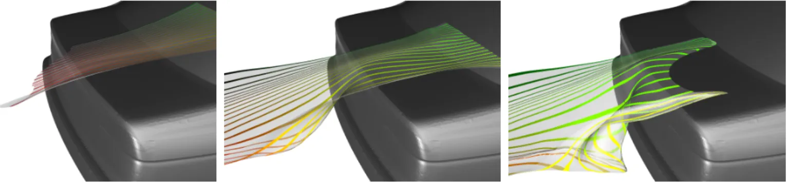
Since this dataset is stationary, streak surfaces with a fixed (constant in time) seeding curve are identical to stream surfaces, and thus our method is computationally more exhaustive than a dedicated stream surface algorithm (e.g. [5]). However, we demonstrate a general-ized streak surface in Figure 6, where the seeding curve is moving downwards parallel to the rear window. Since the complexity of this dataset requires long computation times, such a moving seeding curve possesses exploratory character without involving interactive seeding; here, the region behind the rear window is explored. The surface is textured with a streak stripe pattern. Again, as the streak reaches the lower part of the window, the surface is drawn into the vortex behind the car. While seeding is terminated as the seed curve reaches the lower end of the window, the surface advection is continued, and this illustrates an interesting velocity profile just above the surface of the trunk, and a zone near the window center where the flow moves much slower than further out.
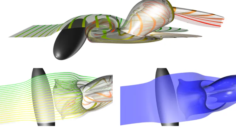
Delta Wing In order to study the effects of vortex breakdown in
aviation, an unsteady simulation of a delta wing configuration exhibit-ing vortex breakdown was performed. We have selected this dataset since it has proven difficult from a numerical perspective in previous work. It represents an ideal numerical test case for the robustness of our method. The dataset consists of several hundred time steps over a grid with 19 million tetrahedral elements. A time surface was seeded above the wing, and parallel to it, near the wing tip. The flow is violent in this area as surrounding air is forced around the wing and twisted into several vortices above the wing. This region of the dataset is very highly resolved; to obtain an accurate surface, 187,645 integral curves had to be traced. Here, the integration time is rather short, but the nu-merical integration scheme has to take very small steps to compute the
Fig. 6. Three frames from an animation showing the evolution of a generalized streak surface in the Car dataset. The surfaces is seeded on a curve moving parallel to the rear window. After seeding is terminated, some parts of the surface remain attached to the rear window. The surface is depicted using a streak ribbon texture.
integral curves. Figure 9 shows the evolution of the surface at early and late stages of evolution. The surface is well resolved, and the right image illustrates the mesh obtained from our algorithm. To provide spatial context, we have applied a striped texture to this time surface, where the stripes indicate radial distance on the seed surface to the wing tip. The surface demonstrates how several vortices are formed and interact near the wing’s leading edge.
8 CONCLUSION
In this work, we have made the following contributions:
• We have presented a novel approach for the computation of time and streak surfaces in large and time-varying datasets. Our ap-proach decouples mesh advection and adaptation from integral curve computation, allowing to achieve optimal precision and performance in the computation of the latter and exploit inherent parallelism.
• To maximize the visualization gain from time and streak surface computation, we make use of a compact representation of the surface evolution that allows full real-time interaction with the temporal component of the surface for visualization.
• We have described several aspects of graphical representation such as transparency and texturing of time and streak surfaces that benefit their visualization, and the visualization of flows us-ing them.
• Furthermore, we have demonstrated and discussed the behavior of our algorithms with respect to robustness, accuracy, and per-formance, and shown it able to approximate very complex sur-faces in large time-varying vector fields.
For future research, we plan to address a number of limitations of our method. In order to enable more interactive seeding, we envision com-puting time and streak surface in an incremental, progressive manner, that quickly generates low quality results from downsampled vector field data; once an interesting surface is found, it may then be com-puted in high quality. To further reduce computation times and gain the ability to treat largest-scale datasets, we plan on exploiting addi-tional parallelization options. Concerning visualization, further ren-dering and texturing options should be explored to give the surfaces even more of an illustrative character.
ACKNOWLEDGMENTS
The authors wish to thank Markus R¨utten from DLR G¨ottingen for supplying some of the data sets treated here and insightful discussion. We are also very much indebted to our colleagues at the Institute for Data Analysis and Visualization and to Xavier Tricoche at Purdue Uni-versity for discussion and feedback. This work was supported by the Director, Office of Advanced Scientific Computing Research, Office of Science, of the U.S. Department of Energy under Contract No. DE-FC02-06ER25780 through the Scientific Discovery through Advanced Computing (SciDAC) program’s Visualization and Analytics Center for Enabling Technologies (VACET).
REFERENCES
[1] L. Bavoli and K. Myers. Order-independent transparency with dual depth peeling.NVIDIA Developer SDK 10, February 2008.
[2] R. E. Bridson.Computational Aspects of Dynamic Surfaces. PhD thesis, Stanford, CA, USA, 2003.
[3] M. Garland and P. S. Heckbert. Surface simplification using quadric error metrics. InProc. ACM SIGGRAPH, pages 209–216, 1997.
[4] C. Garth, H. Krishnan, X. Tricoche, T. Tricoche, and K. I. Joy. Genera-tion of accurate integral surfaces in time-dependent vector fields. IEEE Transactions on Visualization and Computer Graphics, 14(6):1404– 1411, 2008.
[5] C. Garth, X. Tricoche, T. Salzbrunn, and G. Scheuermann. Surface tech-niques for vortex visualization. InProc. VisSym, Symposium on Visual-ization, pages 155–164, May 2004.
[6] E. Hairer, S. P. Nørsett, and G. Wanner. Solving Ordinary Differential Equations I, second edition, volume 8 ofSpringer Series in Computa-tional Mathematics. Springer-Verlag, 1993.
[7] J. P. M. Hultquist. Constructing stream surfaces in steady 3D vector fields. In A. E. Kaufman and G. M. Nielson, editors,Proc. IEEE Vi-sualization 1992, pages 171 – 178, Boston, MA, 1992.
[8] X. Jiao, A. Colombi, X. Ni, and J. Hart. Anisotropic mesh adaptation for evolving triangulated surfaces. InProc. 15th International Meshing Roundtable, pages 173–190. Springer, 2006.
[9] R. S. Laramee, C. Garth, J. Schneider, and H. Hauser. Texture advec-tion on stream surfaces: A novel hybrid visualizaadvec-tion applied to CFD simulation results. InProc. Eurovis 2006 (Eurographics / IEEE VGTC Symposium on Visualization), pages 155–162, 2006.
[10] H. L¨offelmann, L. Mroz, E. Gr¨oller, and W. Purgathofer. Stream arrows: enhancing the use of stream surfaces for the visualization of dynamical systems.The Visual Computer, 13(8):359 – 369, 1997.
[11] P. J. Prince and J. R. Dormand. High order embedded Runge-Kutta for-mulae.Journal of Computational and Applied Mathematics, 7(1), 1981. [12] T. Schafhitzel, E. Tejada, D. Weiskopf, and T. Ertl. Point-based stream
surfaces and path surfaces. InProc. Graphics Interface 2007, pages 289– 296, 2007.
[13] G. Scheuermann, T. Bobach, H. Hagen, K. Mahrous, B. Hamann, K. Joy, and W. Kollmann. A tetrahedra-based stream surface algorithm. InProc. IEEE Visualization 2001, pages 151–158, 2001.
[14] D. Stalling.Fast Texture-Based Algorithms for Vector Field Visualization. PhD thesis, Freie Universit¨at Berlin, 1998.
[15] J. van Wijk. Implicit stream surfaces. InProc. IEEE Visualization 1993, pages 245–252, 1993.
[16] W. von Funck, T. Weinkauf, H. Theisel, and H.-P. Seidel. Smoke sur-faces: An interactive flow visualization technique inspired by real-world flow experiments. IEEE Transactions on Visualization and Computer Graphics, 14(6):1396–1403, 2008.
[17] R. Westermann, C. Johnson, and T. Ertl. A level-set method for flow visualization. InProc. IEEE Visualization 2000, pages 147–154, 2000. [18] A. Wiebel, X. Tricoche, D. Schneider, H. J¨anicke, and G. Scheuermann.
Generalized streak lines: Analysis and visualization of boundary induced vortices. IEEE Transactions on Visualization and Computer Graphics, 13(6):1735–1742, 2007.
Fig. 7. A streak surface in the Ellipsoid dataset as depicted in our interactive visualization tool. The surfaces is seeded upstream of the ellipsoid in the initial timestep and shows a prominent bubble that precedes the vortex formation. Top: Overview; a time line texture provides temporal orientation. Bottom left: Surface textured with streak ribbons. Bottom right: Without texturing, spatial and temporal orientation on the surface is lost.
Fig. 8. Evolution of a time surface in the Ellipsoid dataset. The surface is seeded on rectangle located immediately downstream from the ellipsoid near the temporal beginning of the dataset and illustrates parts of the flow that remain close to the ellipsoid and twist to envelop the nascent vortex system as it forms. A two-dimensional color map helps identify distinct parts of the surface despite heavy overlap.
Fig. 9.Left images:Evolution of a time surface in the delta wing dataset, seeded parallel to the wing tip. The texture provides radial distance stripes to the wing tip for spatial orientation.Right image:Despite numerical difficulties, the surface mesh remains well-conditioned.