MPRA
Munich Personal RePEc Archive
Competitive nonlinear pricing and
bundling
Mark Armstrong and John Vickers
September 2006
Online at
https://mpra.ub.uni-muenchen.de/70/
MPRA Paper No. 70, posted 4 October 2006
Competitive Nonlinear Pricing and Bundling
∗
Mark Armstrong
Department of Economics
University College London
John Vickers
Department of Economics
University of Oxford
September 2006
Abstract
We examine the impact of multiproduct nonlinear pricing on profit, consumer sur-plus and welfare in a duopoly. When consumers buy all their products from one firm (the one-stop shopping model), nonlinear pricing leads to higher profit and welfare, but often lower consumer surplus, than linear pricing. By contrast, in a unit-demand model where consumers may buy one product from onefirm and another product from another firm, bundling generally acts to reduce profit and welfare and to boost con-sumer surplus. In a more general model where concon-sumers may buy from more than onefirm and where consumers have elastic demands for each product, nonlinear pricing has ambiguous effects. Compared with linear pricing, nonlinear pricing tends to raise profit but harm consumer surplus when: (i) demand is elastic, (ii) there is substantial product differentiation, (iii) there is substantial heterogeneity in consumer demand, (iv) consumers face substantial shopping costs when visiting more than onefirm, and (v) a consumer’s brand preference for one product is strongly correlated with her brand preference for another product. Nonlinear pricing is more likely to lead to welfare gains when (i), (ii), (iv) and (v) hold, but (iii) does not.
1
Introduction
Most economic analysis of imperfect competition is based on the assumption of linear pricing, where the price of a combination of purchases from afirm, whether of one or more products, is equal to the sum of the prices of the component parts. While many markets operate on that basis, an increasing number feature nonlinear pricing–for example, discounts for purchases of larger volumes or of more products. In the absence of easy arbitrage, which
∗The support of the Economic and Social Research Council (UK) is gratefully acknowledged. We are
would undermine it, such pricing can be observed in more or less competitive markets as well as in some with market power.
Examples include energy markets, which traditionally were monopolies but are now open to varying degrees of competition. Consumers are often able to buy their gas and electricity from a single supplier or from two suppliers. In each case, consumers typically face nonlinear tariffs, and they will often enjoy an additional discount if they purchase both services from a single supplier. Similarly, consumers nowadays can often source telecommunications, cable television and internet services from a single supplier or from several, and nonlinear pricing and bundling are commonplace. Nonlinear pricing is also to be seen in areas such as air travel (both individual and corporate) and supermarkets, where loyalty schemes have become more prevalent with the advent of electronic point-of-sale information. The economic importance of nonlinear pricing goes wider still. Thus labour contracts may include extra pay for longer tenure, so that a two-period worker gets a better deal than two one-period workers.1 While
the provision of incentives is doubtless a prime reason for such nonlinear wages, the nature of multi-period competition by firms for labour may also be of relevance, and there may be parallels with multi-product competition among firms for consumers.
The aim of this paper is to compare linear and nonlinear pricing in various settings with imperfect (duopoly) competition. We explain why equilibrium nonlinear pricing is better for profit and welfare and worse for consumers than equilibrium linear pricing in some settings, and why the opposite is true in other settings.
There is an extensive literature on nonlinear pricing and bundling.2 In the context of monopoly supply, analyses include Adams and Yellen (1976), McAfee, McMillan, and Whinston (1989), Armstrong (1996), and Rochet and Choné (1998). In particular, the latter two papers demonstrate the complexity of multiproduct nonlinear pricing for a monopolist, and the profit-maximizing tariff can be derived only in a few isolated examples. Whinston (1990) and Nalebuff(2004) have explored aspects of the relationship between (pure) bundling and entry deterrence by an incumbent monopolist. There is also a growing literature on (more or less) competitive nonlinear pricing and bundling by symmetrically-placed firms. For example Spulber (1979), Stole (1995), Armstrong and Vickers (2001) and Rochet and Stole (2002) examine competitive nonlinear pricing in situations in which consumers purchase all products from a single supplier. The latter two papers suggest that marginal-cost pricing often emerges as a nonlinear pricing equilibrium, in which case welfare is boosted whenfirms offer such tariffs compared with linear pricing.3 More generally, a theme in Armstrong and
Vickers (2001) is that when consumers are one-stop shoppers,firms choose socially desirable tariffs if given freedom to do so.
But how reasonable is the assumption that consumers buy all relevant products from
1See, for example, Stevens (2004).
2Armstrong (2006) and Stole (2006) are recent surveys.
3There is no systematic comparison between nonlinear and linear pricing in terms of profit and consumer
surplus in those papers, although Armstrong and Vickers (2001) show when consumers have homogeneous demands that profit rises and consumer surplus falls when two-part tariffs are employed.
a single supplier? The competitive bundling literature, including the contributions by Matutes and Regibeau (1992), Anderson and Leruth (1993), Reisinger (2006) and Thanas-soulis (2006), investigates nonlinear pricing when some consumers wish to buy products from more than one supplier. This line of analysis suggests that bundling tends to harm profit and welfare but to be pro-consumer. It tends to proceed by way of worked examples and assumes that consumers wish to buy only one unit of a product. Moreover, the models make the polar opposite assumption from the one-stop shopping models that consumers face no intrinsic extra “shopping cost” if they buy from more than onefirm. Thus, the literature on competitive nonlinear pricing and bundling has yielded starkly conflicting results about the pros and cons of nonlinear pricing, which our analysis seeks to reconcile.
The rest of the paper, and the main results, can be summarized as follows. Our point of departure in section 2 is a Hotelling model of product differentiation with one-stop shopping and consumers with heterogeneous demands.4 We show that with nonlinear pricing and
all consumers served, the unique symmetric equilibrium of the model has, in effect, two-part tariffs with marginal prices equal to marginal costs. Welfare is maximized with such nonlinear pricing, whereas with linear pricing there is the problem of excessive marginal
prices. Profit is also higher than with linear pricing for two reinforcing reasons that relate to
elasticity of demand and the extent of consumer heterogeneity. Consumer surplus is however typically lower than with linear pricing.
A limitation of this model is the assumption that each consumer patronizes just one
firm. Section 3 examines the possibility of two-stop shopping–where consumers choose on the basis of prices and brand preferences whether to buy from both firms or just one–in a two-dimensional model of product differentiation with inelastic demand.5 Discounts for
joint purchase–mixed bundling–are a general feature of the nonlinear pricing equilibrium, and have a simple characterization. These discounts, however, give rise to the problem of
excessive loyalty, in that there is too much one-stop shopping. Therefore, in contrast to
the one-stop shopping model, welfare is lower when nonlinear pricing is used. Remarkably, the profit and consumer surplus comparisons between linear and nonlinear pricing are also exactly the opposite of those from the one-stop shopping model.
A unifying model, which allows for consumers to have elastic and heterogeneous demands, is analyzed in section 4. With nonlinear pricing permitted and all consumers buying some of both products, there is an equilibrium with efficient two-part tariffs–i.e., with marginal prices equal to marginal costs. Moreover, the fixed elements of the tariffs are precisely the same equilibrium prices, with the same discount for one-stop shopping, as in the model of section 3 with inelastic demand. Therefore, the nonlinear pricing equilibrium, unlike that with linear pricing, is free from the excessive marginal price problem, but it does suffer from the excessive loyalty problem. The models in sections 2 and 3 each had just one of these effects; hence their contrasting results. Perhaps surprisingly, the analysis of competitive
4This develops the models of Armstrong and Vickers (2001, section 4) and Rochet and Stole (2002). 5This develops the model of Matutes and Regibeau (1992).
linear pricing sometimes turns out to be simpler than either (a) monopoly nonlinear pricing or (b) competitive linear pricing.
Section 5 pursues the comparison between linear and nonlinear pricing in terms of five underlying economic influences: (i) demand elasticity, (ii) product differentiation, (iii) con-sumer heterogeneity, (iv) costs of going to more than one supplier, and (v) correlation in brand preferences. Table 1 indicates whether an increase in each of these influences tends to add to or subtract from the merits of nonlinear pricing relative to linear pricing for welfare, profit and consumer surplus.
Welfare Profit Consumers (i) demand elasticity + + — (ii) product differentiation + + — (iii) consumer heterogeneity — + — (iv) shopping costs + + — (v) brand preference correlation + + —
Table 1: Effects on the relative merits of nonlinear pricing
The excessive marginal prices effect becomes more important relative to the excessive loyalty effect–which favours nonlinear pricing in welfare terms–as demand elasticity, prod-uct differentiation, consumer homogeneity, shopping costs and brand preference correlation increase. For example, the excessive marginal prices effect and the excessive loyalty effect respectively increase in importance with more elastic demand (because deadweight welfare loss ‘triangles’ open up) and as shopping costs fall (because more consumers two-stop shop). The direction of effects on profit tends to be the opposite of that on consumer surplus. In respect of (i), (ii), (iv) and (v), the profit effect has the same sign as the welfare effect. But with greater consumer heterogeneity, the relative merits of nonlinear pricing for welfare and consumers tend to be lower. That is because heterogeneity sharpens linear price competition, which is good for consumers and welfare (as the excessive marginal price effect diminishes) but is bad for profit.
Section 6 concludes by suggesting directions for future research on this topic.
2
Nonlinear Pricing and One-Stop Shopping
Suppose there are n ≥ 1 products, each supplied by two firms, denoted A and B. For exogenous reasons, suppose consumers buy all their suppliers from one firm or the other, i.e., consumers are one-stop shoppers. Consumers differ in their brand preference for the two
firms, x, and their preference for the products,θ. The parameter xis uniformly distributed between 0 (where firm A is located) and 1 (where B is located), while θ is independently
distributed according to some distribution functionF(θ).6 Gross utility (excluding transport
costs) is u(θ, q) if a type-θ consumer buys quantities q. Lump-sum transport cost is t per unit of distance. In sum, a type-(x, θ) consumer’s net utility if she buys quantities qA from
firmA in return for payment TA is
u(θ, qA)−tx−TA ,
and if she buys quantities qB from B with payment TB her utility is
u(θ, qB)−t(1−x)−TB .
In the following analysis, we make the important assumption, which is satisfied subject to conditions on willingness-to-pay relative to costs, that all consumers choose to participate in the market with the relevant range of tariffs. Finally, suppose eachfirm has constant unit costci for supplying producti.
Our first result derives the equilibrium nonlinear tariff, which we will use to compare with linear pricing.7,8
Proposition 1 Suppose that over the relevant range of nonlinear tariffs all consumers are served. Then the unique symmetric equilibrium outcome with nonlinear pricing involves
efficient consumption, and a consumer who buys quantities q makes payment
T(q) =t+P
i
ciqi . (1)
Equilibrium industry profit isπN L =t.
Proof. That the cost-based two-part tariffin (1) is an equilibrium was established in Arm-strong and Vickers (2001, Proposition 5). That this tariff induces the unique symmetric equilibrium outcome can be argued by contradiction. Suppose that in an alternative sym-metric equilibrium, industry profit is Π. Suppose further that the equilibrium tariff T(·) does not satisfy ∂
∂qiT(·)≡ ci. Suppose firm A deviates from the candidate equilibrium, and
instead sets the tariffTˆ(q) =Π+Piciqi. A consumer located atx will buy fromfirm A if
v∗(θ)−Π−tx≥v(θ)−t(1−x), where v∗(θ) = max q :u(θ, q)− P i ciqi
6The assumption thatxis uniform is made purely for expositional convenience, and none of the following
results depend on this assumption. Ifxwere instead distributed on[0,1]with densityf(x)which is symmetric aboutx= 12, then subject to regularity conditions onf(·)the following results remain valid if ‘t’ is replaced by ‘t/f(12)’.
7Note that this result need not hold if (i)θ andxare correlated, (ii)firms have different costs, or (iii) if
some consumers do not buy from eitherfirm. See Rochet and Stole (2002) for further details.
8We do not claim that the tariff in (1) is the unique symmetric tariff. For instance, if all consumers
purchased quantities above some positive lower bound, how the tariff is defined for quantities below this lower bound cannot be uniquely determined.
and v(θ) = max q :u(θ, q)−T(q). Let x(θ) = 1 2 + v∗(θ)−Π−v(θ) 2t
be the marginalxconsumer in theθ-segment. ThenA’s deviation profit isEθ[x(θ)]×Π, and
so the deviation is profitable if Eθ[x(θ)]> 12, i.e., if
Eθ[v∗(θ)]>Π+Eθ[v(θ)] .
(Here and elsewhere,Eθ[·]refers to taking expectations with respect toθ using F(θ).)
How-ever, the left-hand side of the above is total surplus with marginal cost pricing, and the right-hand side is total surplus with candidate tariff (which does not always involve mar-ginal cost pricing). Therefore, this inequality is indeed satisfied, and the unique symmetric equilibrium outcome involves marginal-cost pricing.
Consider next the outcome when linear prices are used. Suppose that the type-θconsumer has demand functions qi(θ, p), where p is the vector of linear pricesp = (p1, ..., pn). (These
demands are the quantities q which maximize u(θ, q)−Pni=1piqi.) Let
v(θ, p) = max
q :u(θ, q)−pq
be type-θ consumer surplus with prices p. Let π(θ, p) be type-θ profit, i.e., π(θ, p) ≡
Pn
i=1qi(θ, p)(pi −ci). It is convenient to introduce one further piece of notation: for a
candidate symmetric equilibrium price vectorp, define
s(θ, r)≡v(θ, c+r(p−c)),
where r is a scalar. This allows us to conduct the analysis in terms of the scalar r rather than the vector p. Then s(θ,0) = v(θ, c) and s(θ,1) = v(θ, p). Since v is convex in p, s is convex inr and so srr(θ, r)≥0. Note that
π(θ, c+r(p−c)) = −rsr(θ, r).
In particular π(θ, p) = −sr(θ,1). For p to be a symmetric equilibrium price vector, it is
necessary that r= 1 maximizes a firm’s profit
Eθ ·µ 1 2 + s(θ, r)−s(θ,1) 2t ¶ (−rsr(θ, r)) ¸ .
This has the first-order condition9
πL=Eθ[−sr(θ,1)] =Eθ · srr(θ,1) + (sr(θ,1))2 t ¸ , (2)
9The second-order condition on r is satisfied provided E
θ[srrr(θ,1)] is not strongly negative, which we
where πL is the equilibrium industry profit with linear prices.
Expression (2) implies that
πL=Eθ · srr(θ,1) + (sr(θ,1))2 t ¸ ≥ 1tEθ £ (sr(θ,1))2 ¤ ≥ 1t(Eθ[sr(θ,1])2 = 1 tπ 2 L . (3)
The first inequality follows since srr ≥ 0, and the inequality is strict if consumer demand
is elastic. We can refer to this as the “elasticity” effect. The second inequality follows from Jensen’s inequality. It is strict if there is some consumer heterogeneity (i.e., if the variance of sr(θ,1)is positive); this is the “heterogeneity” effect. Expression (3) shows that
πL≤t =πN L. Hence profits are lower when linear pricing is employed than with nonlinear
pricing.10 The reason for this is a combination of the elasticity and heterogeneity effects,
both of which act in the same direction. (These two effects are discussed in more detail in sections 5.1 and 5.3.)
Clearly, the marginal-cost pricing that is implemented by nonlinear pricing is unambigu-ously beneficial for welfare (as well as for profits, as we have seen). A more subtle issue is the impact of nonlinear pricing on consumer surplus. For a type-θ consumer, the welfare loss of using linear prices relative to nonlinear prices, which we know involves prices equal to marginal costs, is
v(θ, c)−[v(θ, p) +π(θ, p)] =s(θ,0)−s(θ,1) +sr(θ,1).
If consumers have linear demands (or generally when t is small) this welfare loss is 1
2srr(θ,1).
(The reason for this is that with linear demands s(θ, r) is quadratic in r, and so a second-order Taylor expansion about r= 1 is exactly accurate.) In this case, the aggregate welfare gain when firms employ nonlinear pricing is ∆W = 1
2Eθ[srr(θ,1)]. From (3) we see 2∆W =πL− 1 tEθ £ (sr(θ,1))2 ¤ ≤πL− 1 t(Eθ[sr(θ,1)]) 2 =π L− 1 tπ 2 L , i.e., ∆W ≤ 1 2 πL t (t−πL)≤ 1 2(t−πL),
where the second inequality follows from our previous result that πL ≤ t. Therefore, with
linear demands the welfare gain is less than half the gain in industry profit, and so consumers in aggregate are worse offwhen nonlinear tariffs are used.11
We can summarise our analysis of the one-stop shopping model as:
10Note that this profit comparison seems to be valid in an alternative framework in which consumers
incur transport costs on a per-unit rather than a lump-sum basis (at least when transport costs are small), although the analysis is considerably more complicated. For instance, see Proposition 5 in Yin (2004) for analysis with linear demand.
11The result that consumers are worse offwith nonlinear pricing can be established under weaker
assump-tions than linear demand. For example, letζ(θ)be the elasticity for a type-θconsumer of welfare loss relative to the first best with respect to r, evaluated at r = 1. If ζ(θ)>1 for all θ, then the result holds. (With linear demandsζ= 2.)
Proposition 2 Suppose that over the relevant range of tariffs all consumers are served.
Then compared to the outcome with linear pricing, industry profit and total welfare are higher
with nonlinear pricing. In addition, if each consumer’s demand is linear in prices (or if t is
small), consumer surplus is lower with nonlinear pricing.
In the unique symmetric equilibrium with nonlinear pricing, firms use cost-reflective (so efficient) two-part tariffs. The optimal fixed fee (t) in such a tariff balances (i) the firm’s loss of profit on existing consumers against (ii) its gain in profitable consumers from the other firm. Demand per consumer does not change: it is as if consumers had identical inelastic demands. By contrast, if firms are restricted to linear prices, a firm choosing its price(s) will balance (i) against not only (ii) but also (iii) its gain in profit per consumer. Profit per consumer can change for two reasons. First, with elastic demands, lower prices expand demand from each type of consumer. Second, and less obviously, if consumers are heterogeneous, lowering prices can alter the mix of consumer types coming to a firm–in particular by winning proportionately more high demand (hence high profit) consumers than low demand consumers from the other firm. This second reason why average profi t-per-consumer may rise as linear prices are reduced occurs even if consumers have inelastic demands. These two reasons are reflected in the two inequalities in equation (3). They are both reasons why there is more incentive to lower prices–hence why consumers do better– with linear pricing. Yet welfare is higher with nonlinear pricing because there is no marginal price inefficiency. It follows that profits must be higher then too.
3
Bundling and Two-Stop Shopping
In this section we analyze a model of multi-product competition where consumers can “mix-and-match” products from two firms. We assume here that consumers have unit demands. This case is of interest in its own right; it will also provide the key to the more general elastic demand analysis in sections 4 and 5.
3.1
The Framework
Consider a two-dimensional Hotelling model. Two firms, A and B, each offer their own brand of two products, 1 and 2. The location (or brand preference) of a consumer is denoted (x1, x2) ∈ [0,1]2. Let x1 represent a consumer’s distance from firm A’s brand of product 1
andx2 represent a consumer’s distance from the samefirm’s brand of product 2. The density
of (x1, x2) isf(x1, x2)andfirms are symmetrically placed in terms of consumers:
f(x1, x2)≡f(1−x1,1−x2). (4)
The transport cost (or brand preference) parameter is t1 for product 1 and t2 for product
when they source supplies from two firms. This shopping cost might represent the time or cost involved in visiting two shops rather than one, or it might measure a consumer’s perceived cost of dealing with two firms (paying two bills rather than one, for instance). In order to have some two-stop shoppers in equilibrium, it is necessary to constrain the shopping cost not to be too large, and we assume that
z <min{t1, t2} .
If this inequality does not hold, all consumers will choose to buy both items from one firm or the other, and the distinction between bundling and linear pricing vanishes.
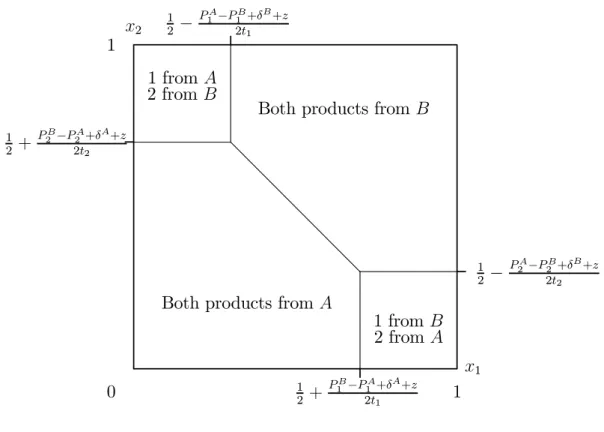
0 1 x1 x2 1 1 2 + PB 2 −P2A+δA+z 2t2 1 2 − PA 1 −P1B+δB+z 2t1 1 2 − PA 2 −P2B+δ B+z 2t2 1 2 + PB 1 −P1A+δ A+z 2t1
Both products fromA
1 fromA
2 from B
1 fromB
2 fromA
Both products fromB
...... ...... ...... ...... ...... ...... ...... ...... ...... ...... ... ... ... ... ... ... ... ... ... ... ... ... ... ... ... ... ... ... ... ... ... ... ... ... ... ... ... ... ... ...
Figure 1: The Pattern of Consumer Demand
Since consumers have unit demand for each product, afirm’s tariffconsists of three prices. LetPi
1 denote firm i’s stand-alone price for its product 1, let P2i be its stand-alone price for
its product 2, and letδi be its discount if a consumer buys both products, so the total charge for buying both products fromfirmiisPi
1+P2i−δ
i. For simplicity, suppose that conditions
in the market are such that all consumers buy both products. The type-(x1, x2) consumer’s
total outlay if she buys both products fromfirmA is P1A+P2A−δ A
+t1x1+t2x2, her total
outlay if she buys both products fromBisPB
1 +P2B−δ
B+t
1(1−x1)+t2(1−x2), and her total
outlay if she buys productifromAand productj 6=ifromB isPA
The consumer located at (x1, x2) will choose the option from among the four possibilities
which involves the smallest outlay. The pattern of demand is as shown in Figure 1.
For simplicity of notation, suppose that production is costless. (This is without loss of generality if marginal costs are constant, and the pricesPiderived below can be considered to
be prices net of marginal costs.) In this case, whenfirms offer the same tariffwith stand-alone prices P1 andP2 and discount (if applicable) δ, industry profit is
(P1+P2)−δ× {proportion of one-stop shoppers} . (5)
In the following analysis, it is useful to introduce some further notation.
0 1 x1 x2 1 1 2 + δ+z 2t2 1 2 − δ+z 2t1 1 2 − δ+z 2t2 1 2 + δ+z 2t1 1 fromA 2 fromB Φ(δ) 1 fromB 2 fromA
Both products from A
Both products from B
Φ(δ) α2 α2 α1 α1 β1, β2 ...... ...... ...... ...... ...... ...... ...... ...... ...... ...... ... ... ... ... ... ... ... ... ... ... ... ... ... ... ... ... ... ... ... ... ... ... ... ... ... ... ... ... ... ...
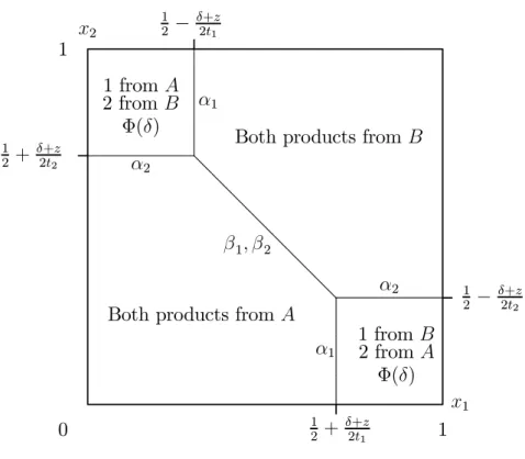
Figure 2: Notation Used in the Analysis Define the (decreasing) function
Φ(δ)≡2 Z 1 2− δ+z 2t1 0 Z 1 1 2+ δ+z 2t2 f(x1, x2) dx2dx1
to be the proportion of consumers who are two-stop shoppers when the firms set the same tariffwhich involves the discount δ. The function Φ summarizes many of the economically-relavant features of this market, and it is depicted on Figure 2. (The symmetry assumption (4) implies that the two rectangles of two-stop shoppers each contain the same proportion of consumers.)
It will be useful to know the derivative of Φ. Write α1(δ) = Z 1 1 2+ δ+z 2t2 f(12 − δ+z 2t1 , x2)dx2 ; α2(δ) = Z 1 2− δ+z 2t1 0 f(x1,12 + δ+z 2t2 ) dx1 (6)
for the line integrals depicted on Figure 2. (From (4), the two integrals markedα1 have the
same value, as do those markedα2.) Then
Φ0(δ) =− µ α1(δ) t1 + α2(δ) t2 ¶ . (7) Finally, write β1(δ) = Z 1 2+ δ 2t2 1 2− δ 2t2 f(12 +t2 t1 (12 −x2), x2) dx2 ; β2(δ) = Z 1 2+ δ 2t1 1 2− δ 2t1 f(x1,12 + t1 t2 (12 −x1)) dx1 (8)
for the line integrals along the diagonal segment depicted on Figure 2. Here, β1 is the
integral in the vertical direction, andβ2 is the integral in the horizontal direction, and they are related byt2β1 =t1β2.
3.2
Linear Pricing
Considerfirst the case wherefirms compete with linear prices–that is to say with no bundling discounts in the present context–so δA = δB = 0. For simplicity, write α0
i = αi(0) and
β0i = βi(0). Suppose the two firms initially set the same pair of linear prices P1 and P2.
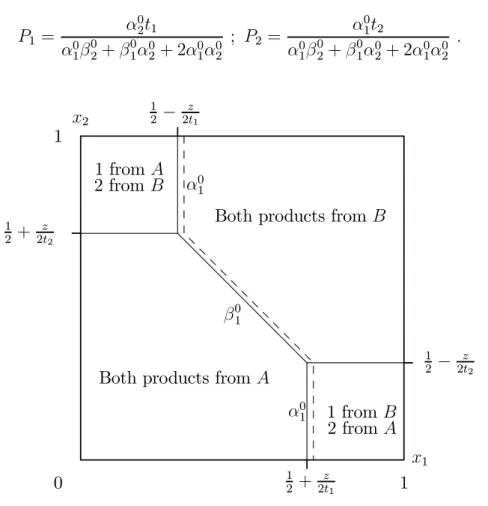
Consider firm A’s incentive to reduce its price P1 by ε, keeping its price for product 2
unchanged at P2. At a symmetric equilibrium, half the consumers buy product 1 from firm
A, and the firm loses revenue ε from each of these infra-marginal consumers. The price reduction shifts the boundary of the set of consumers who buy product 1 from the firm uniformly to the right byε/(2t1), as depicted on Figure 3.
The profit from these marginal consumers is not constant along this boundary. Those consumers on the two vertical boundaries α0
1 on the figure generate profit P1 to the firm,
while those on the diagonal boundaryβ01 generate “double” profit(P1+P2). The total profit
of these marginal consumers is therefore
ε 2t1 × © 2α01P1+β01(P1+P2) ª .
Since the profit gained from the marginal consumers must equal the profit lost from the infra-marginal consumers, it follows that in equilibrium
Similarly, thefirst-order condition for the stand-alone price P2 is
2α02P2+β02(P1+P2) =t2 . (10)
Solving these linear simultaneous equations in(P1, P2)yields explicit formulae for the (unique)
equilibrium prices: P1 = α0 2t1 α0 1β 0 2+β 0 1α02+ 2α01α02 ; P2 = α0 1t2 α0 1β 0 2+β 0 1α02+ 2α01α02 . (11) 0 1 x1 x2 1 1 2 + z 2t2 1 2 − z 2t1 1 2 − z 2t2 1 2 + z 2t1 1 fromA 2 fromB 1 fromB 2 fromA
Both products from A
Both products from B α0 1 β01 α0 1 ...... ...... ...... ...... ...... ...... ...... ...... ...... ...... ... ... ... ... ... ... ... ... ... ... ... ... ... ... ... ... ... ... ... ... ... ... ... ... ... ... ... ... ... ... ... .. ... .. ... .. ... .. ... .. ... .. ... .. ... ... ... ... ... ... ... ... ... ... ... ... ... .. ... .. ... .. ... .. ... .. ... .. ...
Figure 3: Incentive to Reduce Linear Price for Product 1
In most cases, prices and profit falls as the shopping cost z becomes more significant.12
The reason is that, when z is large, the number of consumers (measured by β0i) who are indifferent between buying both products fromAand buying both products fromB increases. These marginal consumers are “doubly profitable” with their two-unit demands. So firms compete hard to attract these consumers, with the result that prices decrease with z.
12For instance, when product preferences x
1 and x2 are independently distributed, the method of proof
for Proposition 6 can show that the sum of the linear prices decreases with z (subject to mild regularity conditions).
It is useful to illustrate these, and subsequent, results by means of a simple example.13
Uniform Example: t1 =t2 =t andf(x1, x2)≡1.
Here,α0 1 =α02 = 12− z 2t andβ 0 1 =β 0
2 = zt. From (11) the equilibrium linear price for each
product is
P1 =P2 =
t2
t+z , (12)
which is decreasing in z. Therefore, with linear pricing the shopping cost makes the market more competitive, in much the same way as firms selling their products with a bundling discount does so.
3.3
Bundling
Suppose next that firms can offer discounts for joint consumption. It turns out that a firm always has a unilateral incentive to do so.
Proposition 3 Suppose the twofirms initially offer the equilibrium linear prices (11). Then
afirm’s profit increases if it unilaterally introduces a small discount δ >0for joint purchase.
Proof. Suppose bothfirms initially offer the linear prices in (11), and consider the effect on
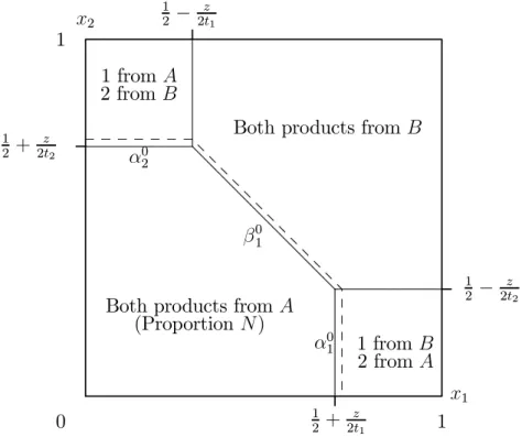
firmA’s profit when it introduces a small joint-purchase discount δ > 0. LetN < 1
2 denote
the proportion of consumers who choose to buy both items from firm A when symmetric linear prices are offered. Here, thefirm loses revenueδfrom theN consumers who previously purchased both products from it in any case, but the discount induces some two-stop shoppers to buy both products from A. See Figure 4.
Specifically, from Figure 4 one sees thatδα01/(2t1)consumers switch from buying product
1 fromB and product2 fromAto buying both from A, and each of these consumers brings in additional profit P1 −δ. Similarly, δα02/(2t2) consumers switch from buying product 1
from A and product 2 from B to buying both from A, and each of these consumers brings additional profit P2−δ. Finally, δβ01/(2t1) consumers switch from buying both items from
B to buying both fromA, and these “doubly profitable” consumers bring profitP1+P2−δ.
In sum, ignoring terms in δ2, the effect on firmA’s profit of introducing the small discount
δ is approximately δα01 2t1 P1+ δα02 2t2 P2+ δβ01 2t1 (P1+P2)−δN =δ(12 −N)>0 .
13This example (withz = 0) wasfirst analyzed by Matutes and Regibeau (1992), and extended in
Arm-strong (2006, section 4.2) to situations where the products were not symmetric in the sense that t1 6= t2.
These earlier analyses took a “brute force” approach by simply calculating the areas of the various regions in Figure 1. This method is only practical when the distribution of (x1, x2) is uniform, and it cannot be
Here, the equality follows from expressions (9)—(10), which proves the result.
This argument is in the same spirit as that used in the monopoly context by McAfee, McMillan, and Whinston (1989).14 However, in our oligopoly framework a firm always has
an incentive to introduce a positive discount, whereas in the monopoly context it was not always the case that a discount was profitable.
0 1 x1 x2 1 1 2 + z 2t2 1 2 − z 2t1 1 2 − z 2t2 1 2 + z 2t1 1 fromA 2 fromB 1 fromB 2 fromA
Both products from A
(ProportionN)
Both products from B
β01 α0 1 α0 2 ...... ...... ...... ...... ...... ...... ...... ...... ...... ...... ... ... ... ... ... ... ... ... ... ... ... ... ... ... ... ... ... ... ... ... ... ... ... ... ... ... ... ... ... ... ... ... ... ... ... ... ... ... ... ... ... ... ... ... ... ... ... ... ... ... ... .. ... .. ... .. ... .. ... .. ... ..
Figure 4: Incentive to Introduce Bundling Discount
An intuition for this result goes as follows. Starting from symmetric equilibrium with linear pricing, there would be nofirst-order effect on the profits of afirm that reduced each of its standalone prices by 12δ for smallδ because those prices are optimal for thefirm (i.e., the envelope theorem applies). Suppose instead that the firm does not change its stand-alone prices but introduces a discountδ for joint purchase. From (4), this brings the same gain in custom for each of the two products as the stand-alone price cuts. But it involves strictly less foregone profit on intra-marginal custom because the discount is restricted to one-stop shoppers rather than all the firm’s consumers. The firm, having been roughly indifferent about the stand-alone price cuts, will therefore strictly gain from the bundling discount. In sum, offer a bundling discount is a more cost-effective way to boost market share than cuts in linear prices.
Notice, however, that if both firms offer the same (small) joint purchase discountδ, each
firm’s profit falls (by approximatelyN δ) compared to the profit generated with linear pricing. This illustrates the prisoner’s dilemma nature of competitive bundling.
0 1 x1 x2 1 1 2 + δ+z 2t2 1 2 − δ+z 2t1 1 2 − δ+z 2t2 1 2 + δ+z 2t1 1 fromA 2 fromB Φ(δ) 1 fromB 2 fromA
Both products from A
Both products from B
Φ(δ) α2 α2 α1 α1 ...... ...... ...... ...... ...... ...... ...... ...... ...... ...... ... ... ... ... ... ... ... ... ... ... ... ... ... ... ... ... ... ... ... ... ... ... ... ... ... ... ... ... ... ... ... ... ... ... ... ... ... ... ... . ... ... . ... ... . ... ... . ... ... . .... ... ... . ... ... . ... ... . ... ... . ... ... . ... ... . ... ... ... ... ... ... ....
Figure 5: Effect of Changing the Bundle Discount
Having established that linear pricing cannot be an equilibrium when firms can offer bundling discounts, we turn next to analysis of the equilibrium nonlinear tariffs. It turns out that there is a simple and general formula for the equilibrium discount δ:
Proposition 4 In a symmetric equilibrium the discount δ satisfies
Φ(δ) + 12Φ0(δ)δ= 0 . (13)
Proof. Suppose that the symmetric equilibrium nonlinear tariff involves the stand-alone price P1 for product 1, the stand-alone price P2 for product 2, and the bundling discount
δ. Consider the effect on firm A’s profit if it increases its discount by a small amount 2ε
and simultaneously increases each of its stand-alone prices byε. The result is that its total charge to one-stop shoppers is unchanged, but the total charge for each two-stop shopping option rises byε. The net effect on thefirm’s profit is depicted in Figure 5, where the two-stop shopping regions shrink to the dashed regions: the deviation moves the upper boundary marked α1 to the left by ε/(2t1) and lower boundary α1 to the right by the same amount;
the upper boundaryα2 is moved up byε/(2t2)and the lower boundaryα2 down by the same
amount. The net effect on firmA’s profit is then approximately (εΦ(δ)) + ε 2t1 α1(P1−δ)− ε 2t1 α1P1+ ε 2t2 α2(P2−δ)− ε 2t2 α2P2 =ε ¡ Φ(δ) +12Φ0(δ)δ¢ ,
where the equality follows from (7). For this deviation to be unprofitable, expression (13) must hold in equilibrium.
A simple corollary of this result is thatδ tends to zero as the shopping costz approaches min{t1, t2}. That is to say, as almost all consumers are anyway one-stop shoppers, there
is little benefit to firms in inducing still more consumers to become one-stop shoppers by means of a bundle discount. In this sense, the shopping cost reduces the incentive to bundle. For instance, in the Uniform Example we have Φ(δ) = 2(12 − δ+2tz)2, and so expression (13)
implies that δ= 12(t−z).
A crucial point is that welfare is reduced when firms offer discounts for joint purchase: there is excessive loyalty, as more consumers than is efficient buy both products from the same firm. The efficient pattern of consumption requires there to be no bundling discount, so that the pattern of demand is as depicted in Figure 3.
By examining Figure 5, one sees that when the discount δ is increased by ε, the extra consumers who buy product 1 from the less preferred firm is equal to α1t1ε, and each of these consumers incurs the extra travel cost(δ+z)compared to buying the product from the closer
firm, although these consumers also save the shopping costz. Thus, their net disutility is δ. Similarly, α2t2ε extra consumers buy product 2 from the less preferred firm, and these each incur a net disutility δ.
In sum, the extra welfare loss caused by increasing δ by ε is
εδ× µ α1 t1 +α2 t2 ¶ =εδ×(−Φ0(δ)).
Denote byw(δ)the level of welfare corresponding to the bundling discountδ relative to the
first-best welfare level (i.e., the welfare level corresponding to the case of linear pricing when
δ= 0). Thus −w(δ) is welfare loss relative to thefirst best. It follows that
w0(δ) =δΦ0(δ) . (14) This condition and w(0) = 0 yield w(δ). For instance, in the Uniform Example we have
Φ(δ) = 2(12−δ+2tz)2 andδ= 12(t−z), in which case (14) implies that the equilibrium welfare loss relative to the case of linear pricing is
(t−z)3
12t2 . (15)
As expected, as the shopping cost becomes large, this welfare loss falls to zero since the bundling discount also falls to zero.
Having derived the equilibrium discount δ as in (13), we can now derive the equilibrium stand-alone prices P1 and P2 in the same way in which the linear prices were derived in
section 3.2. For simplicity, given the equilibrium δ, write αi = αi(δ) and βi = βi(δ). The
pattern of demand is as shown on Figure 6.
0 1 x1 x2 1 1 2 + δ+z 2t2 1 2 − δ+z 2t1 1 2 − δ+z 2t2 1 2 + δ+z 2t1 1 fromA 2 fromB 1 fromB 2 fromA
Both products from A
Both products from B α1 β1 α1 ...... ...... ...... ...... ...... ...... ...... ...... ...... ...... ... ... ... ... ... ... ... ... ... ... ... ... ... ... ... ... ... ... ... ... ... ... ... ... ... ... ... ... ... ... ... .. ... .. ... .. ... .. ... .. ... .. ... .. ... ... ... ... ... ... ... ... ... ... ... ... ... .. ... .. ... .. ... .. ... .. ... .. ...
Figure 6: Incentive to Reduce Stand-Alone Price for Product 1
Consider firmA’s incentive to reduce its stand-alone price P1 byε, keeping its discount
unchanged at δ and its stand-alone price for product 2 unchanged at P2. At a symmetric
equilibrium, half the consumers buy product 1 from firm A, and the firm loses revenue ε
from each of these infra-marginal consumers. The price reduction shifts the boundary of the set of consumers who buy product 1 from the firm uniformly to the right by ε/(2t1). Those
consumers on the upper boundaryα1 on the figure generate profit P1 to the firm, those on
the diagonal boundaryβ1 generate profit(P1+P2−δ), and those on the lower boundaryα1
generate incremental profit (P1−δ).
Since the profit gained from the marginal consumers must equal the profit lost from the infra-marginal consumers, it follows that in equilibrium
α1P1+β1(P1+P2−δ) +α1(P1 −δ) =t1 .
Similarly, thefirst-order condition for the stand-alone price P2 is
Solving these linear simultaneous equations in(P1, P2)yields explicit formulae for the
stand-alone prices, as reported in the next result.
Proposition 5 At a symmetric equilibrium, the discountδ satisfies (13) and the stand-alone prices are P1 = δ 2+ α2t1 α1β2+β1α2+ 2α1α2 ; P2 = δ 2 + α1t2 α1β2+β1α2+ 2α1α2 . (16)
Notice that the stand-alone prices in (16) are uniquely determined given the discount
δ. Then, provided there is a unique solution to the first-order condition for the discount in (13), which can be ensured by assuming regularity conditions on the shape of Φ, there is then only one possible nonlinear pricing equilibrium with some two-stop shoppers.15,16
In the Uniform Example, with the equilibrium discount δ = 12(t − z) it follows that
α1 =α2 = 14 − 4zt andβ1 =β2 = 1
2 +
z
2t. From (16) the equilibrium tariffis then
17 P1 =P2 = 14(t−z) + 2t2 3t+z ; δ= 1 2(t−z) . (17)
Therefore, as in the linear pricing regime, the shopping cost z acts to lower all prices. The reason is the same: the shopping cost expands the margin of “doubly profitable” consumers, which intensifies competition.
3.4
Comparing the Regimes
The regimes of linear pricing and bundling are easily compared in the Uniform Example.
First, notice that as z tends to t, so that the proportion of two-stop shoppers vanishes, the tariffs associated with linear pricing (12) and with bundling (17) converge. That implies that profit, consumer surplus and welfare also converge for large z.
Figure 7 depicts relative profit, welfare and consumer surplus for allz ≤t. The analytic expression for industry profit with bundling is not illuminating, but can be calculated using
15We have not investigated second-order conditions in general for the tariff in Proposition 5, so cannot
be sure that any (pure strategy) equilibria exists. However, we have examined the case of the uniform distribution for(x1, x2), and verified that this tariffis a global best response for onefirm if the rival offers
the same tariff.
16There is always another, less interesting, pure bundling equilibrium. Suppose one firm offers a tariff
involving extremely high stand-alone prices. Then no consumer will ever be a two-stop shopper, and so the rival might as well offer a similar tariff. In the case wheret1=t2=tand(x1, x2)uniformly distributed, one
can show that this pure bundling equilibrium involves setting a price for the bundle equal to t(and setting the stand-alone prices prohibitively high). However, there are good reasons to believe that this second equilibrium is non-robust. For instance, it involves firms playing weakly dominated strategies. Moreover, Thanassoulis (2006) shows that when there are some consumers who wish to buy just one item, this ceases to be an equilibrium.
17The model of Matutes and Regibeau (1992) corresponds to the casez= 0, whenP
expression (5). We depict the bundling profit relative to that with linear pricing (divided by
t) as the thin line in thefigure. Here,z ranges from zero, where the profit loss with bundling relative to linear pricing is about 30%, to t, where profit is the same in the two regimes. In particular, bundling acts to destroy profit relative to linear pricing. The thick line depicts the difference in aggregate consumer surplus (divided byt) in the two regimes, which is positive but decreases to zero as z approachest.18 In particular, consumers in aggregate are always better offin the bundling regime. Finally, the dotted line depicts welfare with bundling (15) relative to linear pricing (divided byt). Of course, welfare falls when bundling is used. For instance, when z = 0 only an eighth of consumers are two-stop shoppers with bundling, whereas maximal efficiency requires that half the consumers should use two suppliers (as occurs with linear pricing).
1 0.75 0.5 0.25 0 0.5 0.25 0 -0.25 -0.5 z/t z/t
Figure 7: The Effect ofz on Profit, Consumer Surplus and Welfare
In this example, the stand-alone price with bundling in (17) is lower than the corresponding linear price in expression (12) wheneverz is sufficiently small.19 In such cases, all prices fall
when bundling is used, and so all consumers benefit. For larger z, the two-stop shoppers are worse offin the bundling regime, although (as shown on thefigure) overall consumer surplus is always higher with bundling.
18Thanassoulis (2006) examines effects of mixed bundling on consumer welfare in a version of this
frame-work where there are some “small” consumers who just want one product. He toofinds that with no extra costs of two-stop shopping mixed bundling is better for consumers and worse forfirms than stand-alone pric-ing, but with (prohibitive) shopping costs the opposite can occur as competition for two-product consumers protects one-product consumers if mixed bundling is disallowed.
Moving beyond this example, it appears to be widely true that aggregate consumer surplus rises, and profit (and of course welfare) falls, when bundling is used. The next result establishes this in the context of independently distributed product preferences, while a simple form of correlated brand preferences is analyzed subsequently.
Proposition 6 Suppose thatx1 andx2 are independently distributed, with respective density
functionsf1(x1)andf2(x2)and respective distribution functionsF1(x1)andF2(x2). Suppose
the distributions satisfy the hazard rate conditions
d dx F1(x) f1(x) ≥ 1 4 ; d dx F2(x) f2(x) ≥ 1 4 (18)
(for x≤ 12). Then compared to the outcome with linear pricing, industry profit and welfare
fall and aggregate consumer surplus rises when bundling is used.
Proof. See appendix.
Before discussing this result in more detail, it is worth checking its robustness to the presence of correlation in brand preferences. In many situations, it is plausible that if a consumer prefersfirmA’s product 1 then she is more likely to prefer the samefirm’s product 2, so that x1 and x2 are correlated. That is to say, firm-level brand preference may be
an important factor in a consumer’s brand preferences over individual products. As is the case with substantial shopping costs, this situation implies that the proportion of two-stop shoppers is smaller than in the uncorrelated case. How does this impact on the incentive to engage in bundling?
In general, the impact of correlation on the bundling discount is not obvious. In rough terms, an increase in correlation will cause there to be fewer consumers in the “north-west” and “south-east” portions of the square, i.e., for the functionΦ(·)to be shifted downwards. However, without further information expression (13) does not indicate what happens to equilibriumδ when Φ is shifted downwards.
For instance, consider the following variant of the Uniform Example.20 For simplicity,
suppose products are symmetric (t1 = t2 = t). Suppose that a fraction ρ of consumers
have perfectly correlated preferences, so thatx1 =x2, and this common brand preference is
uniform on[0,1]. The remaining1−ρconsumers have locations(x1, x2)uniformly distributed
on the unit square. In this example,α0 1 =α02 = (1−ρ)(12− z 2t)andβ 0 1 =β 0 2 = 12−(1−ρ)( 1 2− z t). 21 Therefore,
20A similar framework is used in Nalebuff(2004, section III.C). See Reisinger (2006) for further analysis
of the effect of correlation in a related framework.
21Strictly speaking,β
i(δ)in (8) is not defined in this example, since there is no (two-dimensional) “density”
on the linex2=x1. However, by examining small changes inPias depicted on Figure 3, one can verify that
from (11), the equilibrium linear price for each product is
P1 =P2 =
t2
t+ (1−ρ)z .
Thus, positive correlation acts to relax competition (unless there are no shopping costs, in which case correlation has no impact on linear prices).
1 0.75 0.5 0.25 0 0.5 0.25 0 -0.25 -0.5 correlation correlation
Figure 8: The Effect ofρ on Profit, Consumer Surplus and Welfare
Turning to the case where bundling is employed, Φ(δ)is here equal to2(1−ρ)(12−δ+2tz)2,
and so expression (13) shows that the equilibrium discount does not depend onρand equals
δ = 12(t−z). From (14), the welfare cost of bundling with this discount is just scaled down by the factor (1−ρ), and so from (15) this welfare cost is (1−ρ)(t12−zt2)3. With the discount
δ = 12(t−z), we have α1 =α2 = 41(1−ρ)(1− zt) and β1 =β2 = 1 2 + 1 2(1−ρ) z t. Expression
(16) then shows that the equilibrium bundling tariffis
P1 =P2 = 1 4(t−z) + 2t2 2t+ (1−ρ)(t+z) ; δ = 1 2(t−z) . (19) Thus, like the linear prices, the equilibrium bundling prices are increasing with correlation. The stand-alone prices with bundling are higher than the equilibrium linear prices whenever correlation is sufficiently strong (e.g., when z = 0, stand-alone prices rise with bundling whenever ρ > 13). When there is perfect correlation (or if z = t), there are no two-stop shoppers in equilibrium, and the outcomes with and without bundling coincide.
Figure 8 represents the relative profit (thin line), welfare (dotted line) and consumer surplus (thick line) associated with bundling versus linear pricing (all divided by t), as correlationρvaries. (The shopping costz is set equal to zero in thefigure.) Thus, the profi t-destroying effect of bundling is mitigated, though not overturned, when there is positive correlation. By comparing Figures 7 and 8 we see that effects of increased correlation in product brand preferences is qualitively similar to the effects of increasing the shopping cost. In this model why dofirms do worse, and consumers do better, with nonlinear pricing than with linear pricing? With nonlinear pricing, Propositions 3 and 4 establish that firms will choose to offer discounts to one-stop shoppers. Such discounts can intensify price competition generally so that stand-alone purchases might become cheaper too (or at least they do not rise by enough to overturn the consumer benefits of the discount). When there are discounts for joint purchase, a wider margin of competition for one-stop shoppers opens up–i.e., consumers for whom the operative choice is to buy both products from firm A or both from B. Such consumers are “doubly profitable”; they bring two profit margins (less the discount for joint purchase) so their existence often intensifies price competition generally. Thus larger bundling discounts discounts, by creating more doubly profitable consumers, may strengthen incentives to reduce stand-alone prices as well. (The effect is similar to the impact of the shopping cost z.) Bundling discounts do not necessarily do so, because the discount itself reduces the profit obtained from the doubly profitable consumers. Nonetheless, even when bundling raises the stand-alone prices, the price rise is not (under the conditions of Proposition 6) sufficient the outweigh the consumer benefits of the discount.
Therefore consumers usually do better with nonlinear pricing than with linear pricing, when these effects are lessened. Yet discounts induce the excessive loyalty inefficiency, so depress welfare. It follows that profit is higher with linear pricing.
It is striking that these are exactly the opposite comparative statics to those obtained in the one-stop shopping model presented in Proposition 2. In that model, where demand was elastic, giving greater pricing freedom to firms–in particular the freedom to engage in non-linear pricing–enhanced equilibrium profit and welfare but was detrimental to consumers. But with consumers able to choose between one- and two-stop shopping, and with inelastic demand, giving firms the freedom to offer discounts for joint purchase lowers profit and wel-fare but is good for consumers. We will now analyze a model general enough to encompass and reconcile these contrasting findings.
4
Bundling and Elastic Demand
In this section we extend the unit-demand bundling model to allow consumers to have elastic and heterogenous demands. As well as being of interest for its own sake, the more general model will enable us to explain the sharp contrast between the results from the one-stop shopping model (section 2) and the unit-demand bundling model (section 3).
We make the innocuous assumption that consumers buy all their supplies of a given product from one firm or the other. In general, firm i’s tariff consists of three options:
T1i(q1) is the charge for q1 units of product 1 if the consumer does not buy any product 2
from the firm; Ti
2(q2) is the corresponding tariff if the consumer only buys product 2 from
thefirm, andTi
12(q1, q2)is the tariffif the consumer buys all her supplies from the firm.
Suppose a type-θ consumer has gross utility u(θ, q1, q2) if quantity qi of product i is
consumed. If the type-(θ, x1, x2) consumer buys quantities (q1, q2) from firm A, her net
utility is u(θ, q1, q2)−T12A(q1, q2)−t1x1−t2x2. If she buys quantities (q1, q2) from firm B,
her net utility is u(θ, q1, q2)−T12B(q1, q2)−t1(1−x1)−t2(1−x2). And if she buys quantity
qi of product i from A and quantity qj of product j from B, her utility is u(θ, q1, q2)−
TA
i (qi)−TjB(qj)−tixi −tj(1−xj)−z. The consumer will choose quantities and suppliers
to maximize this utility. As in section 2, suppose that θ is distributed independently from the brand preference parameters (x1, x2). Suppose that eachfirm incurs a marginal cost ci
for serving a consumer with a unit of product i. Finally, suppose that parameters are such that all consumers wish to buy some of each product.
In this model two kinds of inefficiency can arise. First, marginal prices may diverge from marginal costs, and as a result there will be a sub-optimal amount of each product being consumed. This welfare effect was seen with linear pricing in the one-stop shopping analysis of section 2, but not in the basic bundling model of section 3 where the unit demand framework meant that high prices had no welfare impact. This is the excessive marginal price effect. Second, tariffs may encourage excessive one-stop shopping, and consumers may be induced to one-stop shop more often than is socially efficient. This inefficiency was seen in the basic bundling model, but did not arise in the one-stop shopping framework. This is the excessive loyalty effect. In the unified model presented in this section, both inefficiencies can be present. We will see that with linear pricing, inefficiencies arise from excessive marginal prices but not from excessive loyalty, whereas with nonlinear pricing the reverse is true.
4.1
Linear Pricing
Write v(θ, p1, p2) = maxq1,q2u(θ, q1, q2)−p1q1−p2q2 for the consumer surplus of the type-θ
consumer when linear prices are p1 and p2. If both firms set the same linear prices, the
pattern of consumer demand is exactly as depicted on Figure 3. (The θ parameter has no impact on a consumer’s choice of firm when firms offer the same tariff.) In particular, in a symmetric equilibrium there will be no inefficiency due to excessive loyalty, although there will be inefficiency due to excessive marginal prices.
If firm A undercuts B’s product 1 price by ε, this shifts the boundary of the set of type-θ consumers who buy the product from A uniformly to the right by 2εt1q1(θ, p1, p2).
Each of the marginal consumers on the vertical boundaries α0
1 brings extra profit (p1 −
c1)q1(θ, p1, p2), while each “doubly profitable” consumer on the diagonal boundaryβ01 brings
profit (p1−c1)q1(θ, p1, p2) + (p2−c2)q2(θ, p1, p2). Set against this is the impact of the price
1 contribute product 1 profit which is changed byε[q1(θ, p1, p2)+(p1−c1)∂p1∂ q1(θ, p1, p2)], and
in a symmetric equilibrium the proportion of such consumers equals a half. Finally, there is the effect of changing p1 on demand for the firm’s product 2. This is only relevant for
the firm’s one-stop shoppers, who are N in number in equilibrium. Each of these one-stop shoppers generates product 2 profit which is changed byε(p2−c2)∂p1∂ q2(θ, p1, p2).
Putting all this together and taking expectations over θ implies that the first-order con-dition forp1 to be the equilibrium price for product 1 is this generalization of (9):
Eθ £¡ 2α01(p1−c1)q1+β01((p1−c1)q1+ (p2−c2)q2 ¢ q1 ¤ =t1×Eθ · q1+ (p1−c1) ∂q1 ∂p1 + 2N(p2−c2) ∂q2 ∂p1 ¸ . (20) (Here, the dependence of demands qi on p1, p2 and θ has been suppressed.) A similar
ex-pression holds for product 2.
Formula (20) is complex, and reflects the effects of own and cross-price elasticities, con-sumer heterogeneity (via the quadratic terms q2
1 andq1q2), the extent of product diff
erenti-ation, the shopping cost, and correlation in product brand preferences (via the size of N). An extension to the Uniform Example illustrates some of the main effects.
Linear Uniform Example: ti =t; f(x1, x2)≡1; qi(θ1, θ2, p1, p2) =θi(1−bpi); ci = 0.
Thus, demand functions are linear and exhibit no cross-price effects, and consumer het-erogeneity is represented by an idiosyncratic multiplicative termθi. Here, suppose that each
θi has mean 1 and variance σ2, and let the covariance of θ1 andθ2 be κσ2 for −1≤κ ≤1.
It is quite natural to suppose that there is positive correlation in the scale of demands for the two products across consumers (i.e., κ >0), since it is likely that a consumer’s income will be positively correlated with her demand for each product. The parameterbrepresents the sensitivity of demand to marginal price. With a linear pricepfor each product, industry profit is2p(1−bp)and welfare relative to the first best is −bp2.
As in section 3.2,α0 i = 1 2− z 2t andβ 0 i = z
t, and so (20) implies that the equilibrium linear
price for a unit of either product, p, satisfies
p(1−bp)2
1−2bp =
t2
t+z+σ2[t+κz] , (21)
which generalizes (12). This equilibrium price increases withtand falls withz, b, σ2 andκ.22
The impact of these comparative statics, together with their intuition, will be explored in section 5.
22The left-hand side of (21) is increasing inpandbover the relevant range0
≤p≤1/(2b). The right-hand side is increasing int and decreasing inz,σ2 andκ.
4.2
Nonlinear Pricing
In this section we establish that it is an equilibrium for firms to offer tariffs with marginal prices equal to marginal costs, and with fixed charges corresponding to the bundling prices derived in section 3.23
Proposition 7 Suppose that over the relevant range of tariffs all consumers wish to purchase
both products. Then it is an equilibrium for each firm to offer the following tariff:
T1(q1) =P1+c1q1 ; T2(q2) =P2+c2q2 ; T12(q1, q2) =T1(q1) +T2(q2)−δ , (22)
whereP1, P2 and δ comprise the mixed bundling tariff described in Proposition 5.
Proof. See appendix.
Despite the generality of the demand structure and consumer heterogeneity, this equilib-rium is remarkably simple. As with Proposition 1 the shape and heterogeneity of consumer demand functions have no impact on either industry profit or on welfare relative to thefirst best, so long as all consumers participate. (Welfare continues to be determined by expression (14).) In particular, and perhaps surprisingly, whether or not the two products are comple-ments or substitutes in consumer demand makes no difference to the equilibrium incentive to offer bundling discounts. In this equilibrium there is efficient marginal-cost pricing, but there is inefficiency due to excessive loyalty. In this more general model, the impact of non-linear pricing on profit, consumer surplus and welfare is ambiguous. In the next section, we discuss how the various aspects of consumer preferences determine the net impact of nonlinear pricing.
5
Comparing the Regimes
In this section we compare linear pricing and fully flexible nonlinear tariffs.24 At the end of
section 3 we noted the contrast between the model of one-stop shopping (with elastic demand) and the model with consumer choice between one- and two-stop shopping (with inelastic demand) in respect of the consequences for profit, welfare and consumer surplus of allowing
23Notice that, unlike Proposition 1, we have not been able to show that this is the unique symmetric
equilibrium. One reason is the existence of at least one other, pure bundling equilibrium (see footnote 16).
24One could also consider an intermediate regime in whichfirms offer quantity discounts for a particular
product, but cannot offer bundling discounts across products. In welfare (and profit) terms, this pricing regime delivers the best of both worlds, since the excessive loyalty effect and the excessive marginal price effect are both avoided. However, it would be hard for public policy to enforce this intermediate regime, since in practice it is not always clear what constitutes a distinct product. (For instance, should a season ticket to a concert series count as an inter-product or intra-product discount?) For this reason, we focus on the transparent distinction between linear pricing and fullyflexible nonlinear tariffs.
firms freedom to depart from linear pricing. The analysis of the unified model of section 4 now allows us to reconcile these findings and to undertake a more general comparison of linear and nonlinear pricing, and to show the importance of five kinds of economic effect: (i) demand elasticity, (ii) product differentiation, (iii) consumer heterogeneity, (iv) shopping costs, and (v) correlation in brand preferences. The impact of these effects was summarised in Table 1 in the introduction.
5.1
The E
ff
ect of Demand Elasticity
When nonlinear pricing is used, the shape of the demand functions has no effect on profit or welfare (see Proposition 7). With linear pricing, on the other hand, it is plausible that profit and welfare are lower when demand is elastic. For instance, in section 2 we suggested that the “elasticity effect” was one reason why linear prices yielded lower profits than nonlinear prices. As far as the welfare comparison is concerned, linear pricing has the advantage that there is no excessive loyalty inefficiency, but there is the inefficiency due to excessive marginal prices. This may be expected to become more prominent as demand becomes more elastic, because for a given price the welfare loss is larger if demand is more elastic. On the other hand, greater demand elasticity lowers the equilibrium price. However, when consumer demand is sufficiently inelastic, the model is approximated by the unit demand model of section 3, in which case there is no excessive pricing inefficiency and nonlinear pricing harms profit and welfare, but benefits consumers, relative to the case of linear pricing.
0.5 0.375 0.25 0.125 0 0.5 0.25 0 -0.25 -0.5 bb
To explore these elasticity effects further consider the Linear Uniform Example, where the linear price is given by expression (21). With nonlinear pricing, Proposition 7 shows that profit does not depend on the elasticity parameter b. However, in this example at least, profit with linear pricing is decreasing in b. When demand is sufficiently sensitive to price, profit with nonlinear pricing exceeds that with linear pricing. Thus, in the unified model of section 4, the impact of nonlinear pricing on profit is ambiguous.
Figure 9 plots (as the thin solid line) the difference between the profit with nonlinear pricing and with linear pricing as a function of the elasticity term b (here t = 1, z = 0 and
σ2 = 0). The welfare difference between nonlinear and linear pricing is plotted as the dotted
line on thefigure, while the difference in consumer surplus is the thick solid line. Whenb= 0 we return to the unit demand setting, where profit and welfare are reduced with bundling, while consumers benefit. With sufficiently elastic demand, the reverse holds. In this example, welfare is improved by nonlinear pricing even for relatively inelastic demand. Finally, it is worth noting that for intermediate elasticities, both profit and consumer surplus rise with nonlinear pricing. Thus,firms and consumers do not inevitably have opposing interests when it comes to price discrimination.
5.2
The E
ff
ect of Product Di
ff
erentiation
Generally, when (t1, t2) is small, all prices converge to marginal costs, whether linear or
nonlinear pricing is employed, and so the two regimes yield approximately the same profit, welfare and consumer surplus.
0.4 0.3 0.2 0.1 0 0.125 0.1 0.075 0.05 0.025 0 -0.025 -0.05 tt
For instance, consider the Linear Uniform Example. Figure 10 shows relative profit (the thin line), consumer surplus (the thick line) and welfare (the dotted line) associated with nonlinear versus linear pricing as t varies. (Here, b= 1,z = 0 andσ2 = 0.) In this example welfare is–very slightly–reduced by nonlinear pricing when the products offered by the two
firms are close substitutes. This is true quite generally. The reason is that, when z = 0, the excessive loyalty welfare loss is proportional to t,25 while the welfare loss due to excessive marginal prices is of order(t2).26 Thus, for smallt, the welfare losses due to excessive loyalty
will dominate the losses due to excessive pricing, and so nonlinear pricing lowers welfare.27
(The analysis in the next section can show that the separate impact of nonlinear pricing on consumers and profit is ambiguous, even whent is small.) However, Figure 10 indicates that the welfare loss may be rather small. Moreover, this discussion has assumed that exogenous shopping costs are zero. Once z > 0, whenever t becomes sufficiently small, consumers will become one-stop shoppers regardless of whether nonlinear or linear pricing is used. In this case there is no extra welfare cost involved in bundling, and the excessive marginal pricing problem dominates. So nonlinear pricing is then sure to yield higher welfare (as was demonstrated in section 2).
5.3
The E
ff
ect of Consumer Heterogeneity
The discussion in section 2 mentioned the heterogeneity effect, where the presence of con-sumers with different demands acted to intensify linear price competition and to reduce the profit obtained with linear pricing. In this section we explore this in more detail. The reason why consumer heterogeneity acts to depress the equilibrium linear prices can be seen from expression (20). Speaking loosely, a “mean-preserving spread” of the demand functions has no impact on the right-hand side of (20), but it raises the left-hand side via the quadratic terms. The impact of this is similar to a reduction in the product differentiation parameter
t1, which will typically causes prices to fall. The economic intuition is that with
hetero-geneity a price cut attracts proportionally more high demand (hence high profit) consumers from the rivalfirm–so improves, at the margin, themix of consumers (an effect absent with homogeneity). Since prices are then closer to marginal costs, this acts to boost the welfare
25Whenz = 0, the discountδ in (13) and the prices P
i in (16) are homogeneous degree one in(t1, t2).
The pattern of demand illustrated in Figure 5 is unaffected if (t1, t2)are scaled up proportionally, so long
as all consumers continue to buy both products, and so the equilibrium fraction of one-stop shoppers is homogeneous degree zero in(t1, t2). The equilibrium welfare differencewis also homogeneous degree one in
(t1, t2). In particular, whent1=t2=t, the welfare loss is proportional tot.
26With linear pricing price-cost margins are roughly proportional totfor small t, which implies that the
welfare loss from excessive marginal prices is of ordert2.
27The result contrasts with Armstrong and Vickers (2001, Proposition 3), where we argued that price
discrimination led to welfare gains in markets wherefirms offered closely substitutable products. In the earlier paper, we assumed a one-stop shopping framework, so thefirst-order effect of excessive loyalty caused by price discrimination was absent. As a result, the comparison focussed on the second-order effects associated with excessive pricing (which indeed favour price discrimination).