R E S E A R C H A R T I C L E
Open Access
Do little interactions get lost in dark
random forests?
Marvin N. Wright
1, Andreas Ziegler
1,2,3and Inke R. König
1*Abstract
Background: Random forests have often been claimed to uncover interaction effects. However, if and how interaction effects can be differentiated from marginal effects remains unclear. In extensive simulation studies, we investigate whether random forest variable importance measures capture or detect gene-gene interactions. With capturing interactions, we define the ability to identify a variable that acts through an interaction with another one, while detection is the ability to identify an interaction effect as such.
Results: Of the single importance measures, the Gini importance captured interaction effects in most of the simulated scenarios, however, they were masked by marginal effects in other variables. With the permutation importance, the proportion of captured interactions was lower in all cases. Pairwise importance measures performed about equal, with a slight advantage for the joint variable importance method. However, the overall fraction of detected interactions was low. In almost all scenarios the detection fraction in a model with only marginal effects was larger than in a model with an interaction effect only.
Conclusions: Random forests are generally capable of capturing gene-gene interactions, but current variable importance measures are unable to detect them as interactions. In most of the cases, interactions are masked by marginal effects and interactions cannot be differentiated from marginal effects. Consequently, caution is warranted when claiming that random forests uncover interactions.
Keywords: Random forests, Trees, Variable importance, Gene-gene interactions, Epistasis
Background
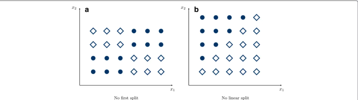
Random forests have often been claimed to uncover inter-action effects [1–8]. This is deduced from the recur-sive structure of trees, which generally enables them to take dependencies into account in a hierarchical man-ner. Specifically, a different behavior in the two branches after a split indicates possible interactions between the predictor variables [9]. However, some variable combi-nations without clear marginal effects might make the tree algorithm ineffective (see Fig. 1). In particular in random forests, it is difficult to differentiate between a real interaction effect, marginal effects and just random variations.
To investigate how random forests deal with interaction effects, we are interested in two aspects. For the first, we *Correspondence: [email protected]
1Institut für Medizinische Biometrie und Statistik, Universität zu Lübeck, Universitätsklinikum Schleswig-Holstein, Campus Lübeck, Ratzeburger Allee 160, 23562 Lübeck, Germany
Full list of author information is available at the end of the article
consider an example reported in the studies by Dro´zdzik et al. [10] and Zschiedrich et al. [11] on a polymorphism in theMDR1gene as a susceptibility factor for Parkinson’s disease. Only a very small marginal genetic effect was shown, but there was a significant interaction between the variant and pesticide exposure on disease risk. Hence, it is of interest whether this genetic variant would nonetheless be identified as a predictor in random forests. If a vari-able is identified by the random forest that contributes to the classification with an interaction effect, this interac-tion effect iscapturedby the model. The second aspect is whether random forests are able to identify the interaction effect per se and the predictor variables interacting with each other. We will use the termdetectfor this in the fol-lowing. Many authors argue that random forests capture interactions [1–5], while others even state that they iden-tify, uncover or detect them [6–8]. However, empirical studies are rare.
It has been shown that variable importance measures are, in principle, suitable to capture interactions [12, 13].
© 2016 Wright et al.Open AccessThis article is distributed under the terms of the Creative Commons Attribution 4.0 International License (http://creativecommons.org/licenses/by/4.0/), which permits unrestricted use, distribution, and reproduction in any medium, provided you give appropriate credit to the original author(s) and the source, provide a link to the Creative Commons license, and indicate if changes were made. The Creative Commons Public Domain Dedication waiver (http://creativecommons.org/publicdomain/zero/1.0/) applies to the data made available in this article, unless otherwise stated.
a b
Fig. 1Problematic splits for classification trees and random forests. In (a) no reasonable first split on the variablesx1orx2can be made. However,
two subsequent splits onx1andx2split the data perfectly. In (b), again no reasonable first split is possible, even though the classes are linear
separable. Both the variablesx1orx2have to be considered simultaneously and even with several subsequent splits onx1andx2, no accurate
classification is possible
However, current methods seem to fail in high dimen-sional data [14], and the effect of various different inter-action models on importance measures has not been investigated. To detect interactions, the standard variable importance measures of random forests, Gini and permu-tation importance, are by design not suitable. Therefore, different methods specifically designed to detect effects of pairs of variables in random forests were proposed [15–17]. These methods measure a joint variable impor-tance to rank variable pairs by their interaction effects. The efficacy of these approaches has only been inves-tigated in small simulations and without considering marginal effects or different interaction scenarios.
In an extensive simulation study, we therefore investi-gate whether random forests variable importance mea-sures capture or detect interactions effects. In the first part, the Gini and permutation variable importance mea-sures are used to capture interaction effects between single nucleotide polymorphisms (SNPs). Since these methods cannot detect interaction effects, we consider only the pairwise importance measures in the second part, in which we focus on the detection of interacting SNPs. In our simulation, we consider various interaction mod-els, vary effect sizes, minor allele frequencies (MAF) and the number of SNPs randomly selected as splitting can-didates (mtry). Even though SNPs are used as predictive variables, all results naturally generalize to other kinds of categorical data.
Methods
Random forests
Detailed descriptions of random forests are available in the original [18] and more recent literature [19, 20]. In brief, random forests are ensembles of decision trees. Depending on the outcome, trees can be classification or regression trees (CARTs) [21], survival trees [22] or prob-ability estimation trees (PETs) [23], among others. For
random forests, a number of trees are grown that differ because of two components. First, each tree is based on a prespecified number of bootstrap samples or subsamples of individuals. Second, only a random subset of the vari-ables is considered as splitting candidates at each split in the trees. To classify a subject in the random forest, the results of the single trees are aggregated in an appropri-ate way, depending on the type of random forest. A great advantage of random forests is that the bootstrapping or subsampling for each tree yields subsets of observa-tions, termed out-of-bag (OOB) observaobserva-tions, which are not included in the tree growing process. These are used to estimate the prediction performance or variable impor-tance. There are two specifically important parameters to random forests: The numbermtryof randomly selected splitting candidates is usually kept fixed for all splits. In most implementations, the default value formtryis√p, wherepis the number of variables in the dataset. How-ever, for datasets with a large number of variables, a larger value is required to capture more relevant variables [3]. Typically, mtryis tuned, e.g. by comparing the predic-tion performance of several values using cross validapredic-tion. Another important parameter of random forests is the size of single trees. This size is usually controlled by stopping the tree growth if a minimal terminal node size is reached. For regression and survival outcomes, the terminal node size is usually tuned together with themtryvalue, while for classification the trees are grown to purity.
Gini importance
The standard splitting rule in random forests for classifi-cation outcomes is to maximize the decrease of impurity that is introduced by a split. For this, the impurity is typ-ically measured by the Gini index [21]. Since a large Gini index suggests a large decrease of impurity, a split with large Gini index can be considered to be important for classification. Thus, the Gini importance for a variablexi
in a tree can be computed by summing the Gini index val-ues of all nodes in which a split onxihas been conducted.
The average of all tree importance values forxi is then
termed Gini importance of the random forest forxi. In our
simulation studies, theRpackageranger[24] was used to compute the Gini importance.
Permutation importance
The basic idea of the permutation variable importance approach [18] is to consider a variable important if it has a positive effect on the prediction performance. To evalu-ate this, a tree is grown in the first step, and the prediction accuracy in the OOB observations is calculated. In the second step, any association between the variable of inter-estxiand the outcome is broken by permuting the values
of all individuals for xi, and the prediction accuracy is
computed again. The difference between the two accuracy values is the permutation importance forxifrom a single
tree. The average of all tree importance values in a random forest then gives the random forest permutation impor-tance of this variable. The procedure is repeated for all variables of interest. The packageranger[24] was used in our analyses.
Pairwise permutation importance (PPI)
To measure the permutation importance for a pair of variables, a modification of the permutation importance was proposed [15]. Instead of permuting a single variable, two variablesxi andxj are permuted simultaneously. As
for the standard permutation importance, the difference in prediction accuracy with and without permutation is computed and used as importance value for the respec-tive pair of variables. This procedure is repeated for all variable pairs of interest. Here, usually, only a subset of the variable pairs is selected to reduce runtime. Although the concept could easily be extended to higher orders of interaction, this would lead to high computational costs. Originally, the approach was implemented inFORTRAN 77[15]. For easier usage and higher computational speed, we included the PPI measure in theRpackageranger
[24] (see Additional file 1 for a version including this measure).
Joint importance by maximal subtrees (JMST)
The joint importance by maximal subtrees measure ([17], JMST) is based on maximal subtrees introduced by Ishwaran et al. [16]. For this, any subtree of the original tree is called anxi-subtree if the root node is split byxi. A
subtree is a maximal subtree if it is not a subtree of a larger xi-subtree. It can now be assumed that variables with
sub-trees closer to the root node have a larger impact on the prediction and are therefore more important than oth-ers. The distance of the maximal subtree to the root node is termed the minimal depth of a variable and gives the
importance value. For interactions, second-order maximal (xj,xi)-subtrees are used that are defined as the maximal xj-subtree within a maximal xi-subtree. Here, the
mini-mal depth is the distance of the maximini-mal (xj,xi)-subtree
to the root of the maximalxi-subtree. For the simulation
studies, thefind.interactionfunction of theR
pack-agerandomForestSRC[25] was used with the option
maxsubtree. A matrix with normalized minimal depths
for all pairs of variables of interest is returned. Since we are interested in two-way interactions, we used the aver-age of the minimal depths of (xj,xi) and (xi,xj)-subtrees to
compute the joint importance ofxiandxj.
Joint variable importance (JVIMP)
For the joint variable importance measure ([16], JVIMP), maximal subtrees are utilized again. As in permutation importance, the association between a variablexiand the
outcome is broken by randomization. However, instead of permuting the variable, a so-called noise-up procedure is employed: Each observation is dropped down the tree until a maximalxi-subtree is reached. From then on, all
further splits are replaced by random child node assign-ments. This is repeated for all trees. The importance of variable xi is now measured by the difference between
the OOB prediction accuracy of the noised-up forest and the original forest. For pairs of variables xi and xj, the
random assignments start as soon as a maximal subtree of xi or xj is reached. The importance of the
interac-tion effect ofxi andxjis computed by the difference of
the sum of both single importance values (additive effect) and the joint importance value (pairwise effect). The
find.interactionfunction ofrandomForestSRC
[25] was used with the optionvimp.
Genetic interaction models
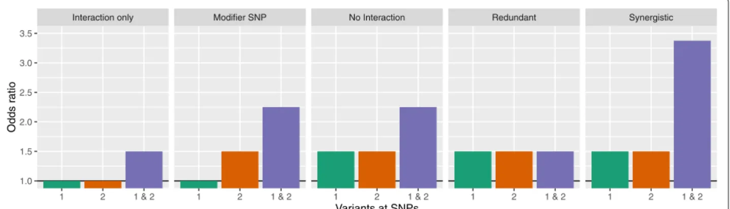
We considered two-way interactions between two SNPs based on 5 interaction models. The models were adopted from Lanktree & Hegele [26] but modified for gene-gene instead of gene-environment interactions and illustrated in Fig. 2. First, in Interaction only, both SNPs have no marginal effects, i.e. an odds ratio (OR) of 1, but an inter-action effect. Second, inModifier SNP, only one SNP has a marginal effect, but the increase for the combination of both is larger than would be expected from marginal effects only. InNo interaction, both SNPs have marginal effects, but there is no additional interaction effect. In the Redundant model, both SNPs have marginal effects, but the combination leads to no further increase in the OR. Finally, inSynergistic, both SNPs have a marginal effect and an additional interaction effect in the same direction.
Simulation studies
Based on these 5 interaction models, data was simu-lated with varying effect sizes for the interaction effects
Interaction only Modifier SNP No Interaction Redundant Synergistic 1.0 1.5 2.0 2.5 3.0 3.5
1 2 1 & 2 1 2 1 & 2 1 2 1 & 2 1 2 1 & 2 1 2 1 & 2
Variants at SNPs
Odds r
atio
Fig. 2Interaction models. Odds ratios for different interaction models, depending on a variant at the first SNP only, the second SNP only or at both SNPs. If both SNPs have no marginal effect, i.e. an odds ratio of 1, but an effect if variants are present at both SNPs, the model is calledInteraction only. If only one SNP has a marginal effect and the combined effect is larger than the single marginal effect, the SNP without marginal effect is a
Modifier SNP. InNo interactionboth SNPs have a marginal effect but no additional combined effect. In this example both SNPs have an odds ratio of 1.5 and the combined effect is exactly 1.52=2.25. If both SNPs have a marginal effect and the combined effect is as large as each single marginal
effect, the marginal effects do not add up and we call the modelRedundant. If both SNPs have a marginal effect and the combined effect is larger than expected by the marginal effects only, it is aSynergisticmodel
and marginal effects and different MAF values. In each dataset, two interacting SNPs with marginal and/or inter-action effects depending on the interinter-action model, 5 marginal-only SNPs and 93 noise SNPs were generated. Data was simulated with a sample size of 1000. The phe-notypes were simulated with additive effects and logit models, depending on the interaction model (Table 1). The effects were chosen out of βM = (0.4, 0.8) and
βI = (0.4, 0.8), for marginal and interaction effects, respectively. The baseline β0 was chosen to generate an approximate equal number of cases and controls for each scenario. The MAF wasMAFM =(0.2, 0.4)andMAFI = (0.2, 0.4) for the marginal effect and interaction SNPs, respectively. For the noise SNPs, the MAF was drawn from a uniform distribution between 0 and 1. All simu-lation parameters are presented in Table 2. The resulting
Table 1Logit model generation
Interaction model SNP1 SNP2 SNP1 x SNP2 Interaction only 0 0 βI Modifier SNP 0 βI βI No interaction βI βI 0 Redundant βI βI −βI Synergistic βI βI βI
In the simulation studies, 2 interacting SNPs and several SNPs having only marginal effects or no effects (noise SNPs) were generated. The phenotypes were simulated with additive effects and logit models. The interacting SNPs have marginal and/or interaction effects, depending on the genetic model. All effects of the interacting SNPs are generated from a single coefficientβI. The table shows marginal effects of
SNP1 and SNP2 and the interaction effect. If variants at both SNPs are present, the resulting effect is the sum of the marginal effects and the interaction effect. The baselineβ0was chosen to generate an approximate equal number of cases and controls for each scenario
penetrance table forβI = 0.4 andMAFI = 0.4 is shown
in Table 3 for theInteraction onlymodel, the penetrance tables for all other interaction models and scenarios are given in the Additional file 2 (Tables S1–S20).
To study the influence of the fixed parameters, we fur-ther simulated datasets where the number of marginal-only SNPs was reduced to 2 and datasets where the number of noise SNPs was increased to 2493. In both cases, the effects were fixed toβM = βI = 0.4 and the MAF toMAFM =MAFI =0.2. To investigate the impact
of linkage disequilibrium (LD), we simulated LD struc-tures based on data from phase 3 of the 1000 genomes project [27]. A random region on chromosome 22 was chosen, and 1000 SNPs without missing data and a MAF between 0.05 and 0.2 were selected. The mean pairwise LD between these SNPs was D = 0.69 (SD 0.35) and the correlationr2 = 0.14 (SD 0.23). For each simulated dataset, 100 SNPs were randomly selected out of these region, and new data with LD structure was simulated using HapSim [28]. Effects ofβM = βI = 0 and all com-binations of βM = (0.4, 0.8) and βI = (0.4, 0.8) were simulated.
On each dataset, random forests with 500 trees each were grown with a varying number of SNPs randomly selected as splitting candidates (mtry value), chosen from (10, 50). To investigate the capture of interacting SNPs, two measures of importance for single variables were computed in the first part, the Gini importance and the permutation importance. Second, to investigate the detection of interactions, we computed the pairwise importance measures PPI [15], JMST [17] and JVIMP [16]. In total, 800 simulation scenarios were analyzed, and for each scenario, we ran 100 replications. Using every
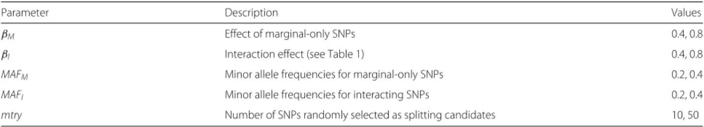
Table 2Simulation parameters
Parameter Description Values
βM Effect of marginal-only SNPs 0.4, 0.8
βI Interaction effect (see Table 1) 0.4, 0.8
MAFM Minor allele frequencies for marginal-only SNPs 0.2, 0.4
MAFI Minor allele frequencies for interacting SNPs 0.2, 0.4
mtry Number of SNPs randomly selected as splitting candidates 10, 50
All combinations of these parameters were simulated. The interaction modelsInteraction only,Modifier SNP,No interaction,RedundantandSynergistic(see Fig. 2) were considered. As variable importance measures, we determined the Gini importance, permutation importance, pairwise permutation importance, joint importance by maximal subtrees and joint variable importance, resulting in a total of 800 simulation scenarios. In addition, one simulation with only 2 marginal-only SNPs and one simulation with 2493 noise SNPs was performed. In both cases,mtry=50,βM=βI=0.4 andMAFM=MAFI=0.2 was set. Finally, a simulation with simulated linkage disequilibrium was performed, see theMethodssection for a description. All simulation scenarios were replicated 100 times
importance measure, the variables were ranked, and the ranks of the true interaction SNPs or, in case of the pair-wise measures, their combination were saved. Inspired by Lunetta et al. [12] and McKinney et al. [29], the propor-tion of replicates in which both true interacpropor-tion SNPs were among the topk ranks is plotted fork = 2,. . ., 10 for the single variable importance measures. A high value for k =2 means that the interacting SNPs are ranked before all other SNPs and the interaction is captured by the ran-dom forest. High values fork = 3,. . ., 10 indicate that the interaction is still captured, but masked by marginal effects or noise.
For the pairwise measures, we plot the proportion of replicates in which the combination of the true interact-ing SNPs was among the topkranks for k = 1,. . ., 10. To make the analyses computationally feasible, combi-nations containing noise SNPs were excluded from the ranking. Here, a high value for a smallkindicates a high proportion of detection of the true interaction, with the exception of theNo interactionmodel, where the interac-tion effect is 0 and any detecinterac-tion would be a false positive result. To compare the ranking of the interacting SNPs with the marginal-only SNPs the proportion of replicates, in which the single variable importance measures ranked the 5 marginal-only SNPs among the topkranks is shown fork= 5,. . ., 15. For the pairwise importance measures,
Table 3Penetrance table for modelInteraction only,βI=0.4,
MAFI=0.4.A1andB1represent the major alleles andA2andB2
the minor alleles
SNP 1
A1A1 A1A2 A2A2
B1B1 0.35 0.35 0.35
SNP 2 B1B2 0.35 0.44 0.54
B2B2 0.35 0.54 0.72
Compared with Table 1 it can be seen that a variant at both SNPs is required for a penetrance larger than the baseline of 0.35. Since the phenotype is simulated with an additive model, the penetrance is increased if two minor alleles are present at one SNP. The penetrances for other models and parameters are computed analogously and are shown in Tables S1–S20 (Additional file 2)
the proportion of replicates, in which all 10 combinations of marginal-only SNPs are among the topkpairs, is shown for k = 10,. . ., 20. Replication code for all simulation studies is included in Additional file 3.
Results
Capturing interaction effects by single variable importance measures
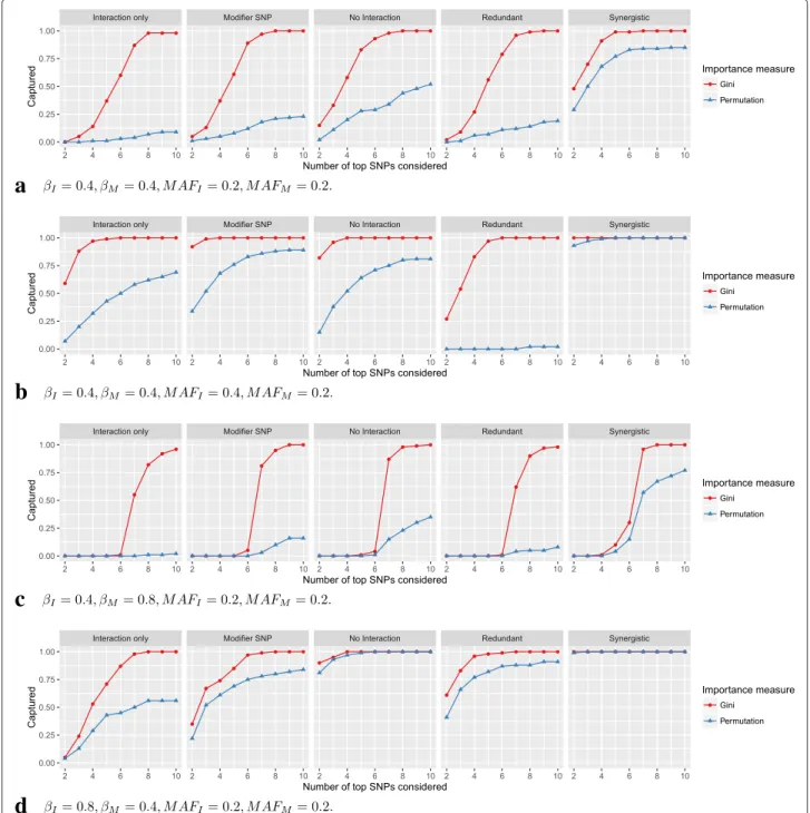
The results for the single variable importance measures and mtry = 50 are shown in Fig. 3. The Gini impor-tance ranked the interacting SNPs generally higher than the permutation importance. However, the results varied greatly, depending on the interaction model, the simula-tion scenario and the importance measure. For moder-ate interaction and marginal effects and equal MAF for interacting and marginal-only SNPs (Fig. 3a), the inter-acting SNPs were ranked in the top 7 by Gini impor-tance in almost all cases. Comparison with the ranking of marginal-only SNPs (Figure S49, Additional file 4) reveals that most of the other top ranked SNPs were marginal-only. However, some noise SNPs were also included. With permutation importance, the fraction of captured interac-tions was generally low, except in theSynergisticmodel. Both importance measures achieved a higher capture frac-tion in No interaction than in Interaction only, which was expected, since these measures were not designed to detect interactions. When the MAF of the interact-ing SNPs was increased (Fig. 3b), the capture fraction was higher for both importance measures and all inter-action models, except for permutation importance and the Redundant model, where the interacting SNPs were almost never ranked in the top 10 SNPs. If instead the MAF of the marginal-only SNPs was increased (Figure S3, Additional file 4), the Gini importance ranked the inter-acting SNPs between the marginal-only and the noise SNPs in almost all cases. For permutation importance, the results were mostly unchanged. If the effect size of the marginal-only SNPs was increased (Fig. 3c), the Gini importance again ranked the interacting SNPs between the marginal-only and the noise SNPs in almost all cases, while the capture fraction of the permutation importance
a
b
c
d
Fig. 3Simulation results for single variable importance measures. On the vertical axis, the proportion of simulation replications in which both interacting SNPs were included in the topkSNPs according to the ranking by the variable importance measures is shown. On the horizontal axis, the number ofktop SNPs considered is shown. If the importance measure included both interacting SNPs in the topkSNPs, they werecaptured. In (a) to (d), different simulation scenarios are shown. The parametersβIandβMcorrespond to the effects of the interacting SNPs and marginal-only SNPs, respectively.MAFIandMAFMare the minor allele frequencies of the corresponding SNPs. See Figures S1–S24 (Additional file 4) for results of all simulation scenarios for the single variable importance measures
was very low, except for the Synergistic model. If the effect size of the interacting SNPs was increased (Fig. 3d), the capture fraction was generally higher compared with Fig. 3a, in particular for the permutation importance. If MAF and effect sizes were modified at the same time, the
described effects added up (Figures S5–S12, Additional file 4). For mtry = 10, which is the default value in most random forests implementations, the capture frac-tion was generally lower (Figures S13–S24, Addifrac-tional file 4). If the number of marginal-only SNPs was reduced
to 2 (Figure S97, Additional file 4), the results were mostly similar, except that, as expected, the interacting SNPs were ranked on average 3 ranks higher. If the number of SNPs was increased to 2500 (Figure S98, Additional file 4) and in the case of LD (Figures S99–S103, Additional file 4), the capture fraction was low with both importance mea-sures. In the simulation with LD, the permutation impor-tance ranked the interacting SNPs higher in most of the scenarios.
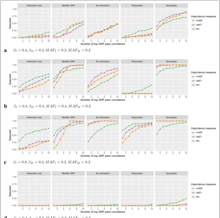
Detecting interaction effects by pairwise variable importance measures
The results for the pairwise variable importance measures and mtry = 50 are shown in Fig. 4. The detection fraction was low in all models. The difference between the methods were generally smaller than for the single variable importance measures. For moderate interaction and marginal effects and equal MAF for interacting and marginal-only SNPs (Fig. 4a), the importance measures were about equal, except for Redundant, where JVIMP was slightly higher, and forSynergistic, where it was lower. Remarkably, with all importance measures, the detection in No interaction was higher than in Interaction only. When the MAF of the interacting SNPs was increased (Fig. 4b), the detection increased for all models, except forRedundant, where it was lower for JMST and PPI and unchanged for JVIMP. In Interaction only, the increase was largest, and for JVIMP, the detection was higher than in No interaction. If instead the MAF of the marginal-only SNPs was increased (Figure S27, Additional file 4), the detection was slightly lower than in Fig. 4a, in par-ticular for JVIMP. If the effect size of the interacting SNPs was increased (Fig. 4c), the detection was higher for all importance measures. The detection of JVIMP was high forInteraction onlyand low forNo interactionand Synergistic. If the effect size of the marginal-only SNPs was increased (Fig. 4d), the detection was very low in all cases. If MAF and effect sizes were modified at the same time, the described effects added up (Figures S29– S36, Additional file 4). Again, for mtry = 10, the detection fraction was generally lower (Figures S37– S48, Additional file 4). If the number of marginal-only SNPs was reduced to 2 (Figure S104, Additional file 4), the results were similar for small values of k, and the detection was higher for larger values of k. This was expected, since combinations including noise variables are excluded in the pairwise measures and thus only 6 combinations of SNPs are possible in this case. If the number of SNPs was increased to 2500 (Figure S105, Additional file 4), the results were comparable to the sim-ulation with 100 SNPs. In the case of LD (Figures S106– S110, Additional file 4), the detection fraction for larger values of k was slightly increased. However, this was also the case if no interaction or marginal effects were
included, indicating that correlations were detected as interactions.
Discussion
In our extensive simulation studies, we found that random forests are capable of capturing SNP-SNP interactions, i.e. of including them in the model. Of the single variable importance measures, the Gini importance ranks the interacting SNPs higher than the permuta-tion importance. The single importance measures are unable to detect interactions, and this by design. They can thus not differentiate between marginal and inter-action effects. But since, in most cases, the interact-ing SNPs are ranked higher than noise SNPs even if no marginal effects are present, we conclude that the interaction effects are thereby captured in ran-dom forests. In general, the ranking depends heavily on the MAF, with more frequent SNPs being ranked higher.
The results of the pairwise importance measures sug-gest that they are unable to detect interactions in the presence of marginal effects. With all measures, marginal effects were detected as interaction effects, and true inter-actions were not found if other SNPs with strong marginal effects were present. Again, SNPs were ranked higher if the MAF was increased. All methods ranked the inter-acting SNPs higher in the model without interaction, compared with the model with interaction only, sug-gesting that interaction effects cannot be differentiated from marginal effect. Of the compared methods, JVIMP [16] achieved the best results, since detection was high-est for the model with interaction only and lowhigh-est for the model without interaction in most of the simulation scenarios.
To study SNP-SNP interactions with random forest, we used 5 interaction models in a simplified setting. We simulated rather strong effects and large MAF values. Our results show that the pairwise impor-tance measures are unable to detect interactions in this setting. In simulations with an increased number of noise SNPs, the single importance measures per-formed worse and the pairwise measures about equal. If LD was considered, only very strong effects were detected at all and again marginal effects were detected as interactions.
Despite the difficulty of the pairwise variable impor-tance measures to detect interactions, our data suggest that interaction effects are generally captured by ran-dom forests. One approach to improve the detection rate might be to use random forests to perform a variable selection first and applying another method to identify interactions subsequently [30, 31]. However, interaction effects might again be masked by marginal effects in that approach. A related idea is to uncover marginal
a
b
c
d
Fig. 4Simulation results for pairwise variable importance measures. On the vertical axis, the proportion of simulation replications in which the true interaction between the two interacting SNPs is included in the topkSNP pairs according to the ranking by the variable importance measures is shown. On the horizontal axis, the number ofktop SNP pairs considered is shown. If the importance measure included the true interaction in the topkSNP pairs, the interaction isdetected. In (a) to (d), different simulation scenarios are shown. The parametersβIandβMcorrespond to the effects of the interacting SNPs and marginal-only SNPs, respectively.MAFIandMAFMare the minor allele frequencies of the corresponding SNPs. See Figures S25–S48 (Additional file 4) for results of all simulation scenarios for the single variable importance measures
effects in a first step and project the remaining effects on a space orthogonal to the marginal effects, to detect interactions in a second step [32, 33]. On a different route, the detection of interactions might be facilitated by developing new pairwise importance measures based on standard random forests [34]. However, it is argued
that in the case of many predictor variables, it is unlikely that interacting variables are selected simultaneously in a given tree [9]. Second, for combinations of variables, the attributable risk [35] can be small, in particular for variants with small MAF. This means that only a small proportion of cases is attributable to the interaction, and
even for large effect sizes these interactions are difficult to detect. Finally, it can be argued that random forests are by design unable to split on interactions [36]. As shown in Fig. 1a, if interacting variables have no marginal effect at all, no first split is possible and the interaction can-not be captured. To solve this, the tree growing process in the random forest itself could be modified to better incorporate interactions. A promising, yet computation-ally intensive new approach are reinforcement learning trees [37], which employ reinforcement learning in each node, to additionally incorporate future splits down in the tree. Several other approaches have been proposed [38], but these are based on single trees only, limiting their usage to low dimensional settings. With fast ran-dom forest implementations now available for large sam-ple sizes [39] and high dimensional data [24] these or new methods could be integrated into the random forest framework.
Conclusions
We conclude that random forests are generally capable of capturing SNP-SNP interactions, but current variable importance measures are unable to detect them. The Gini importance performs better than the permutation importance in identifying SNPs involved in an interac-tion. However, both methods are not designed to uncover interactions as such, and consequently, in most of the cases, the interactions are masked by other SNPs with marginal effects. None of the pairwise importance mea-sures is able to reliably detect interactions. Marginal effects are detected as interaction effects and here, too, other SNPs with marginal effects hinder the detection of interactions. As a result one should be cautious when claiming that random forests uncover interaction effects.
Availability of data and materials
The software and simulation code supporting the conclu-sions of this article are included within the article and its additional files.
Additional files
Additional file 1:Software package. Version of the software package ranger, including the pairwise permutation importance measure. (GZ 39.9 kb)
Additional file 2:Supplementary tables. Penetrance tables for all genetic interaction models, effect sizes and minor allele frequencies. (PDF 78.1 kb)
Additional file 3:Simulation code. Replication material for all simulation studies. (ZIP 44 kb)
Additional file 4:Supplementary figures. All results for the single and pairwise variable importance measures. (PDF 1105 kb)
Competing interests
The authors declare that they have no competing interests.
Authors’ contributions
MNW performed the simulation studies, implemented the pairwise permutation variable importance method and drafted the manuscript. IRK conceived of the study and edited the manuscript. MNW, AZ and IRK contributed to interpretation and presentation of the results. All authors read and approved the final manuscript.
Acknowledgements
This work was supported in part by the German Federal Ministry of Education and Research (BMBF) within the framework of the e:Med research and funding concept (grant 01ZX1313A-2014), the German Centre for Cardiovascular Research (DZHK; Deutsches Zentrum für Herz-Kreislauf-Forschung) and the European Union FP7 project BiomarCaRE (HEALTH-F2-2011-278913).
Author details
1Institut für Medizinische Biometrie und Statistik, Universität zu Lübeck, Universitätsklinikum Schleswig-Holstein, Campus Lübeck, Ratzeburger Allee 160, 23562 Lübeck, Germany.2Zentrum für Klinische Studien, Universität zu Lübeck, Universitätsklinikum Schleswig-Holstein, Campus Lübeck, Lübeck, Germany.3School of Mathematics, Statistics and Computer Science, University of KwaZulu-Natal, Pietermaritzburg, South Africa.
Received: 12 January 2016 Accepted: 21 March 2016
References
1. McKinney BA, Reif DM, Ritchie MD, Moore JH. Machine learning for detecting gene-gene interactions: a review. Appl Bioinforma. 2006;5(2): 77–88.
2. Hastie T, Tibshirani R, Friedman JJH. The Elements of Statistical Learning, 2nd edn. New York: Springer; 2009.
3. Goldstein BA, Polley EC, Briggs FBS. Random forests for genetic association studies. Stat Appl Genet Mol Biol. 2011;10(1):32. 4. Liu C, Ackerman HH, Carulli JP. A genome-wide screen of gene–gene
interactions for rheumatoid arthritis susceptibility. Hum Genet. 2011;129(5):473–85.
5. Grömping U. Variable importance assessment in regression: linear regression versus random forest. Am Stat. 2009;63(4):308–19. 6. Yang P, Hwa Yang Y, Zhou BB, Zomaya AY. A review of ensemble
methods in bioinformatics. Curr Bioinform. 2010;5(4):296–308. 7. Moore JH, Asselbergs FW, Williams SM. Bioinformatics challenges for
genome-wide association studies. Bioinformatics. 2010;26(4):445–55. 8. Touw WG, Bayjanov JR, Overmars L, Backus L, Boekhorst J, Wels M, van Hijum SAFT. Data mining in the life sciences with random forest: a walk in the park or lost in the jungle? Brief Bioinform. 2013;14(3):315–26. 9. Boulesteix A-L, Janitza S, Hapfelmeier A, Van Steen K, Strobl C. Letter to
the Editor: On the term ’interaction’ and related phrases in the literature on random forests. Brief Bioinform. 2015;16(2):338–45.
10. Dro´zdzik M, Białecka M, My´sliwiec K, Honczarenko K, Stankiewicz J, Sych Z. Polymorphism in the P-glycoprotein drug transporter MDR1 gene: a possible link between environmental and genetic factors in Parkinson’s disease. Pharmacogenetics. 2003;13(5):259–63.
11. Zschiedrich K, König IR, Brüggemann N, Kock N, Kasten M, Leenders KL, Kosti´c V, Vieregge P, Ziegler A, Klein C, Lohmann K. MDR1 variants and risk of Parkinson disease. Association with pesticide exposure? J Neurol. 2009;256(1):115–20.
12. Lunetta KL, Hayward LB, Segal J, Van Eerdewegh P. Screening large-scale association study data: exploiting interactions using random forests. BMC Genet. 2004;5(1):32.
13. Garcá-Magariños M, López-de-Ullibarri I, Cao R, Salas A. Evaluating the ability of tree-based methods and logistic regression for the detection of SNP-SNP interaction. Ann Hum Genet. 2009;73(3):360–9.
14. Winham SJ, Colby CL, Freimuth RR, Wang X, de Andrade M, Huebner M, Biernacka JM. SNP interaction detection with random forests in high-dimensional genetic data. BMC Bioinforma. 2012;13(1):164. 15. Bureau A, Dupuis J, Falls K, Lunetta KL, Hayward B, Keith TP,
Van Eerdewegh P. Identifying SNPs predictive of phenotype using random forests. Genet Epidemiol. 2005;28(2):171–82.
16. Ishwaran H. Variable importance in binary regression trees and forests. Electron J Stat. 2007;1:519–37.
17. Ishwaran H, Kogalur UB, Gorodeski EZ, Minn AJ, Lauer MS. High-dimensional variable selection for survival data. J Am Stat Assoc. 2010;105(489):205–17.
18. Breiman L. Random forests. Mach Learn. 2001;45(1):5–32.
19. Boulesteix A-L, Janitza S, Kruppa J, König IR. Overview of random forest methodology and practical guidance with emphasis on computational biology and bioinformatics. WIREs Data Mining Knowl Discov. 2012;2(6): 493–507.
20. Ziegler A, König IR. Mining data with random forests: current options for real-world applications. WIREs Data Mining Knowl Discov. 2014;4(1):55–63. 21. Breiman L, Friedman J, Olshen RA, Stone CJ. Classification and
Regression Trees. Boca Raton: CRC Press; 1984.
22. Ishwaran H, Kogalur UB, Blackstone EH, Lauer MS. Random survival forests. Ann Appl Stat. 2008;2(3):841–60.
23. Kruppa J, Liu Y, Biau G, Kohler M, König IR, Malley JD, Ziegler A. Probability estimation with machine learning methods for dichotomous and multicategory outcome: Theory. Biom J. 2014;56(4):534–63. 24. Wright MN, Ziegler A. ranger: A fast implementation of random forests
for high dimensional data in C++and R. J Stat Softw. 2016. In press. 25. Ishwaran H, Kogalur UB. randomForestSRC: Random forests for survival,
regression and classification. 2014. R package version 1.5.5, http://CRAN. R-project.org/package=randomForestSRC.
26. Lanktree MB, Hegele RA. Gene-gene and gene-environment interactions: new insights into the prevention, detection and management of coronary artery disease. Genome Med. 2009;1(2):28.
27. The 1000 Genomes Project Consortium. An integrated map of genetic variation from 1092 human genomes. Nature. 2012;491:56–65.
28. Montana G. HapSim: a simulation tool for generating haplotype data with pre-specified allele frequencies and LD coefficients. Bioinformatics. 2005;21(23):4309–11.
29. McKinney BA, Crowe JE, Guo J, Tian D. Capturing the spectrum of interaction effects in genetic association studies by simulated evaporative cooling network analysis. PLoS Genet. 2009;5(3):1000432. 30. Meng Y, Yang Q, Cuenco KT, Cupples LA, DeStefano AL, Lunetta KL. Two-stage approach for identifying single-nucleotide polymorphisms associated with rheumatoid arthritis using random forests and Bayesian networks. BMC Proc. 2007;1(Suppl 1):56.
31. Jiang R, Tang W, Wu X, Fu W. A random forest approach to the detection of epistatic interactions in case-control studies. BMC Bioinforma. 2009;10(Suppl 1):65.
32. Pashova H, LeBlanc M, Kooperberg C. Boosting for detection of gene-environment interactions. Stat Med. 2013;32(2):255–66. 33. Sariyar M, Hoffmann I, Binder H. Combining techniques for screening
and evaluating interaction terms on high-dimensional time-to-event data. BMC Bioinforma. 2014;15(1):58.
34. Ziegler A, DeStefano AL, König IR, Bardel C, Brinza D, Bull S, Cai Z, Glaser B, Jiang W, Lee KE, Li CX, Li J, Li X, Majoram P, Meng Y, Nicodemus KK, Platt A, Schwarz DF, Shi W, Shugart YY, Stassen HH, Sun YV, Won S, Wang W, Wahba G, Zagaar UA, Zhao Z. Data mining, neural nets, trees–problems 2 and 3 of Genetic Analysis Workshop 15. Genet Epidemiol. 2007;31(Suppl 1):51–60.
35. Ziegler A, König IR, Pahlke F. A Statistical Approach to Genetic Epidemiology: Concepts and Applications, with an E-learning platform, 2nd edn. Weinheim: Wiley; 2010.
36. Biau G, Devroye L, Lugosi G. Consistency of random forests and other averaging classifiers. J Mach Learn Res. 2008;9:2015–33.
37. Zhu R, Zeng D, Kosorok MR. Reinforcement learning trees. J Am Stat Assoc. 2015;110(512):1770–84.
38. Loh WY. Fifty years of classification and regression trees. Int Stat Rev. 2014;82(3):329–48.
39. Seligman M. Rborist: Extensible, parallelizable implementation of the random forest algorithm. 2015. R package version 0.1-0, http://CRAN.R-project.org/package=Rborist.
• We accept pre-submission inquiries
• Our selector tool helps you to find the most relevant journal
• We provide round the clock customer support
• Convenient online submission
• Thorough peer review
• Inclusion in PubMed and all major indexing services
• Maximum visibility for your research Submit your manuscript at
www.biomedcentral.com/submit