Sobol' indices for problems defined in non-rectangular domains

Contents lists available at ScienceDirect

Reliability

Engineering

and

System

Safety

journal homepage: www.elsevier.com/locate/ress

Sobol’

indices

for

problems

defined

in

non-rectangular

domains

S.

Kucherenko

_,

_O.V.

_Klymenko

_,

_N.

_Shah

a

r

t

i

c

l

e

i

n

f

o

Keywords:

Globalsensitivityanalysis Sobol’ sensitivityindices Dependentinputs

Constrainedglobalsensitivityanalysis Non-rectangulardomain

a

b

s

t

r

a

c

t

AnoveltheoreticalandnumericalframeworkfortheestimationofSobol’ sensitivityindicesformodelsinwhich inputsareconfinedtoanon-rectangulardomain(e.g.,inpresenceofinequalityconstraints)isdeveloped.Two numericalmethods,namelythequadratureintegrationmethodwhichmaybeveryefficientforproblemsoflow dimensionalityandtheMC/QMCestimatorsbasedontheacceptance-rejectionsamplingmethodareproposedfor thenumericalestimationofSobol’ sensitivityindices.Severalmodeltestfunctionswithconstraintsareconsidered forwhichanalyticalsolutionsforSobol’ sensitivityindiceswerefound.Thesesolutionswereusedasbenchmarks forverifyingnumericalestimates.Themethodisshowntobegeneralandefficient.

© 2017TheAuthors.PublishedbyElsevierLtd. ThisisanopenaccessarticleundertheCCBYlicense.(http://creativecommons.org/licenses/by/4.0/) 1. Introduction

The high complexity of models in physics, chemistry, engineering and other fields results in the increased uncertainty in model parameters and model structures. Uncertainty in inputs is reflected in uncertainty of model outputs and predictions. Uncertainty and sensitivity analysis have been recognized as an essential part of model applications. Global sensitivity analysis (GSA) offers a comprehensive approach to model analysis by quantifying how the uncertainty in model output is appor- tioned to the uncertainty in model inputs [1,2]. Unlike one-at-a-time approach, GSA estimates the effect of varying a given input (or set of in- puts) while all other inputs are varied as well, thus providing a measure of interactions among variables. GSA is used to identify key parameters whose uncertainty most affect the variation of the model output of in- terest. This information then can be used to rank variables, fix unessen- tial variables and thus decrease problem dimensionality. Variance-based methods also known as Sobol’ sensitivity indices have become very pop- ular among practitioners due to its efficiency and ease of interpretation [3,4]. Most of the developed techniques for GSA are designed under the hypothesis that inputs are independent. However, in many cases there are dependencies among inputs, which may have significant impact on the importance results.

There have been a number of attempts to extend GSA to models with dependent inputs. We present a brief survey of only the most recent and easy-to-follow developments. Xu and Gertner [5]suggested to split the contribution of an individual input to the uncertainty of the model output into two components: the correlated contribution and the un- correlated one. A regression-based method was used for estimating the correlated and uncorrelated contributions of the inputs. The approach

∗_{Correspondingauthor.}

E-mailaddresses:[email protected],[email protected](S.Kucherenko).

developed originally only for linear models was later extended to non- linear models [6]. Li et al. [7]proposed a generalization of the ANOVA- HDMR decomposition by including covariances to the model variance. They distinguished between structural and correlative contributions of a given input. This method presents some critical issues such as non- uniqueness of the functional decomposition and hence difficulties in in- terpreting the results.

A novel approach for the estimation of Sobol ’ sensitivity indices for models with dependent variables using generalizations of direct Sobol ’ formulas was developed in Kucherenko et al. [8]. Both the main effect and total sensitivity indices were derived as generalizations of Sobol ’ sensitivity indices. Formulas and Monte Carlo (MC) numerical estima- tors similar to Sobol ’ formulas were proposed. A Gaussian copula-based approach was used for sampling from arbitrary multivariate probability distributions. The generalization does not involve the use of surrogate models, data-fitting procedures or orthogonalization of the input factor space.

Mara and Tarantola [9]introduced a set of sensitivity indices which relies on orthogonalisation of correlated inputs. The computation of sen- sitivity indices was performed using a parametric method, specifically the polynomial chaos expansion. Mara et al. [10]extended the develop- ment of sensitivity indices suggested in [9] by proposing two sampling strategies for non-parametric, numerical estimation using the Rosenblatt transformation (RT) [11]. RT, and hence values of sensitivity indices, is not unique: for a model with n inputs there are n! possibilities corre- sponding to all possible permutations of the elements of the input vec- tor 𝑥=(𝑥1,...,𝑥𝑛). The authors considered only the RT obtained after circularly reordering the set ( x1, ..., xn), resulting in n RT transforma- tions. The authors also established the link with the indices proposed by Kucherenko et al. [8]. W.Hao et al. [12] suggested a detailed interpre-

http://dx.doi.org/10.1016/j.ress.2017.06.001

Received8June2016;Receivedinrevisedform1June2017;Accepted4June2017 Availableonline6June2017

tation of indices proposed in [8]. Taking a quadratic polynomial model with normal inputs as an illustration, they derived explicit expressions for sensitivity indices and considered contributions to the values of sen- sitivity indices from all components.

In this work we propose GSA formulations for an even wider class of problems with dependent variables, namely for models involving inequality constraints (which naturally leads to the term ‘constrained GSA ’ or cGSA). Such constraints impose structural dependences between model variables in addition to potential correlations between them. This implies that the parameter space may no longer be considered as an n-dimensional hypercube or hyperrectangle as considered within GSA so far, but may assume any shapes (including disconnected domains) depending on the number and nature of constraints. This class of prob- lems encompasses a wide range of situations encountered in the natu- ral sciences, engineering, design, economics and finances where model variables are subject to certain limitations imposed e.g. by conservation laws, geometry, costs, quality constraints etc. Some examples of such problems are discussed in [13]. An important particular case within this paradigm corresponds to imposing a minimum (maximum) threshold for the model output, i.e., f( x1, ..., xn) ≥fmin, in which case the constraint function can be defined as 𝑔(𝑥1,...,𝑥𝑛)=𝑓(𝑥1,...,𝑥𝑛)−𝑓minand the cor- responding constraint as g( x1, ..., xn) ≥0.

The development of efficient computational approaches for cGSA is challenging because of the potentially arbitrary shape of the feasible do- main of the model variables ’ variation, thus requiring the development of special MC or quasi MC (QMC) sampling techniques and approaches for computing sensitivity indices. This becomes especially difficult for models of high dimensionality. Another challenge consists of analyzing and interpreting model variance and sensitivity indices in such domains, since in this case sensitivity indices will carry structural information im- posed by model constraints. The interpretation of sensitivity indices in such circumstances is crucial for the efficient design of experiments as well as for potential model reduction by fixing or eliminating nonessen- tial variables.

In this paper we have developed and tested several approaches for the numerical estimation of main effect and total sensitivity indices (as defined in [1]) in the cGSA setting. It is organized as follows: the next Section presents formulas for the main effect and total sensitivity indices for models with dependent variables and acceptance–rejection method which can be used to avoid sampling from conditional distri- butions. Section3 considers numerical aspects of the method, namely it presents general MC estimators, acceptance-rejection estimation of Sobol ’ sensitivity indices using grid quadrature formulas and MC esti- mators. Section4presents the application of the proposed methodology to three test cases. Numerical and analytical results are compared and the convergence rates of the MC and QMC methods are discussed. Fi- nally, conclusions are presented in the last Section.

2. Variance-basedsensitivityindicesformodelswithdependent inputs

2.1. Mainandtotaleffectformulaforinputsdefinedinnon-rectangular domainΩn

Consider a model function f( x1, ..., xn) defined in Rn. The input vec- tor 𝑥=(𝑥₁,...,𝑥_𝑛) consists of real-valued random variables with a con- tinuous joint probability distribution function (pdf) p( x₁, ..., x_n). It is assumed that f( x1, ..., xn) has a finite variance. Consider an arbitrary subset of the variables 𝑦=(𝑥_𝑖1,...,𝑥_𝑖𝑠), 1 ≤ s<n and a complementary subset 𝑧=(𝑥_𝑖

𝑠+1,...,𝑥𝑖𝑛), so that 𝑥=(𝑦,𝑧).

The ratio 𝑆𝑦=𝐷𝑦[𝐸̄𝑧(𝑓(𝑦,̄𝑧))]

𝐷 (1)

is known as the main effect index of the subset y. The quantity 𝑆𝑇

𝑦 =

𝐸𝑧[𝐷̄𝑦(𝑓(̄𝑦,𝑧))]

𝐷 (2)

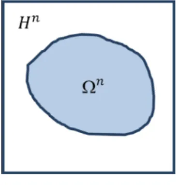
Fig. 1. DomainΩn_⊂Hn_.

is known as the total effect index of the subset y. Collectively Sy, 𝑆_𝑦𝑇are known as Sobol ’ indices in the case of independent inputs. We keep the same definitions for the case of dependent inputs, although meanings of these two indices can be different from those defined in the case of in- dependent inputs (further details are given in Section2.4). In this paper our notations follow closely those of Kucherenko et al. [8].

𝐸̄𝑧(𝑓(𝑦,̄𝑧)) in Eq.(1)denotes a conditional expectation with respect to z with y being fixed and 𝐷̄𝑦(𝑓(̄𝑦,𝑧)) in (2) is a conditional variance with respect to y with z being fixed. D is the total variance. We use notations z and ̄𝑧 (correspondingly y and ̄𝑦) to distinguish a random vector z (correspondingly y) generated from a joint pdf p( y,z) and a random vector ̄𝑧 (correspondingly ̄𝑦) generated from a conditional pdf 𝑝(𝑦,̄𝑧|𝑦)(correspondingly 𝑝(̄𝑦,𝑧|𝑧)).

A formula for the main effect index can be explicitly written as 𝑆_𝑦= 1 𝐷 [ ∫_𝑅𝑠𝑝(𝑦)𝑑𝑦 [ ∫_𝑅𝑛−𝑠𝑓(𝑦,̄𝑧)𝑝(𝑦,̄𝑧|𝑦)𝑑̄𝑧 ]2 −𝑓₀2 ] . (3)

Here 𝑓0=𝐸𝑥(𝑓(𝑥)), p( y) is the marginal pdf of subset of inputs y. This is the so-called double loop formula (DL) [1]. It can be transformed into a different formula which in some cases can be more efficient [8]: 𝑆_𝑦 = 1 𝐷 [ ∫_𝑅𝑛𝑓(𝑦 ′_,𝑧′_)𝑝(𝑦′_,𝑧′_)𝑑𝑦′_𝑑𝑧′ [ ∫_𝑅𝑛−𝑠𝑓(𝑦 ′_{,̂𝑧)𝑝(𝑦}′_,̂𝑧|𝑦′_)𝑑̂𝑧 − ∫_𝑅𝑛𝑓(𝑦,𝑧)𝑝(𝑦,𝑧)𝑑𝑦𝑑𝑧 ]] . (4)

The following notation is used: z,z′ are two different random vectors generated from the joint pdf p( y,z), a random vector ̂𝑧is generated from a conditional pdf 𝑝(𝑦′_,̂𝑧|𝑦′_).

A formula for computing the total effect index 𝑆𝑇

𝑦 (2)can be written as 𝑆𝑇 𝑦 = ₂1_{𝐷 ∫} 𝑅𝑛+𝑠[𝑓(𝑦,𝑧)−𝑓(̄𝑦 ′_,𝑧)]2_{𝑝(𝑦,𝑧)𝑝(}̄𝑦′_{,𝑧|𝑧)𝑑𝑦𝑑}̄𝑦′_{𝑑𝑧. (5)} We note that for the case of independent inputs this formula was suggested in [14].

Consider the situation when the variation of model inputs is sub- ject to an inequality constraint (or a finite number thereof) of the form g( x1, ..., xn) ≥ 0 giving rise in general to an arbitrary (not necessarily connected) domain Ω𝑛={(𝑥1,...,𝑥𝑛)∶𝑔(𝑥1,...,𝑥𝑛)≥0}⊂ 𝑅𝑛Fig.1. De- spite the apparent complication of the problem of evaluating sensitivity indices due to the introduction of constraints, the above formulas for main effect and total sensitivity indices remain to be applicable in any domain Ωn_⊂Rn_{. The only modification required in Eqs.(3)–(5) is the} replacement of pdf’s with those defined in Ωn, which we denote in the following with a superscript ′ Ω′ (e.g. 𝑝Ω_{(𝑦,𝑧)).}

For simplicity, in the following we assume that the model function f( x₁, ..., x_n) is defined in the unit hypercube Hn _{(in the general case} this can be achieved by applying a corresponding coordinate transfor- mation to the original model variables) while the permissible domain

Ωnis enclosed by Hn_:Ωn_⊂Hn_. 219

2.2. Transformationfromconditionaltojointandmarginaldistributions We assume that there is a known procedure for the generation of vectors ( y,z) from a joint pdf 𝑝Ω_{(𝑦,𝑧) defined in a non-rectangular do-} main Ωn_{, which means in particular that 𝑝}Ω_{(𝑦,𝑧) ≡0, ∀( y,z) ∉Ω}n_{. Com-} putation of Sy and 𝑆_𝑦𝑇 requires also sampling from conditional pdf’s. Consider generation of a vector (𝑦,̄𝑧) for the evaluation of 𝑓(𝑦,̄𝑧) from a conditional probability distribution function 𝑝Ω_{(𝑦,̄𝑧|𝑦). Using the ax-} iom of conditional probabilities 𝑝Ω_{(𝑦,̄𝑧|𝑦)𝑝}Ω_(𝑦)=𝑝Ω_{(𝑦,𝑧), 𝑝}Ω_{(𝑦,̄𝑧|𝑦) can} be transformed as

𝑝Ω_{(𝑦,̄𝑧|𝑦)=} 𝑝Ω(𝑦,𝑧)

𝑝Ω_(𝑦) . (6)

Using similar transformations for 𝑝Ω_(𝑦′_,̂𝑧|𝑦′_{)and 𝑝}Ω_(̄𝑦′_{,𝑧|𝑧)formulas}

(3)–(5) for S_yand 𝑆𝑇

𝑦 in domain Ωncan be presented as follows

𝑆_𝑦= 1 𝐷 [ ∫Ω𝑠𝑝 Ω_{(𝑦)𝑑𝑦} [ ∫Ω𝑛−𝑠 𝑓(𝑦,𝑧) 𝑝Ω_(𝑦)𝑝 Ω_{(𝑦,𝑧)𝑑𝑧} ]2 −𝑓₀2 ] , (7) 𝑆_𝑦= 1 𝐷 [ ∫Ω𝑛 𝑓(𝑦′_,𝑧′_)𝑝Ω_(𝑦′_,𝑧′_)𝑑𝑦′_𝑑𝑧′ [ ∫Ω𝑛−𝑠 𝑓(𝑦′_,̄𝑧) 𝑝Ω_(𝑦′₎𝑝 Ω_(𝑦′_{,̄𝑧)𝑑̄𝑧} − ∫Ω𝑛𝑓 (𝑦,𝑧)𝑝Ω(𝑦,𝑧)𝑑𝑦𝑑𝑧 ]] , (8) 𝑆𝑇 𝑦 =₂1_{𝐷 ∫} Ω𝑛 ∫Ω𝑠 [𝑓(𝑦,𝑧)−𝑓(𝑦′,𝑧)]2𝑝Ω(𝑦,𝑧)𝑝 Ω_(𝑦′_,𝑧) 𝑝Ω_(𝑧) 𝑑𝑦𝑑𝑦 ′_{𝑑𝑧. (9)}

Here the lower-dimensional integrals are understood in the sense that ∫Ω𝑠𝐹(𝑦,𝑧)𝑑𝑦=∫(𝑦,𝑧)∈Ω𝑛𝐹(𝑦,𝑧)𝑑𝑦 and ∫Ω𝑛−𝑠𝐹(𝑦,𝑧)𝑑𝑧=

∫(𝑦,𝑧)∈Ω𝑛𝐹(𝑦,𝑧)𝑑𝑧for any F( y,z) ∈L1( Ωn).

The usefulness of these formulas is based on the ability to sample from the joint pdf 𝑝Ω_{(𝑦,𝑧)in Ω}n_{. Although there is a technique based on} the sequential sampling from an inverse cumulative distribution based on RT presented in AppendixA, it has a limited applicability. In the next section we present a more general approach based on the acceptance – rejection method.

2.3. Acceptance– rejectionmethod

Consider the joint pdf p( y,z) in the absence of constraints in Hn_{. We} assume that constraining the variables to an area Ωn_⊂Hn_{implies that} their joint pdf becomes 𝑝Ω_{(𝑦,𝑧), which takes zero values in H}n_{\ Ω}n_and is proportional to p( y,z) within Ωn. Formally

𝑝Ω_(𝑦,𝑧)=

{

𝑝(𝑦,𝑧)∕̄𝐼, (𝑦,𝑧)∈ Ω𝑛

0, (𝑦,𝑧)∉ Ω𝑛. (10)

Here ̄𝐼 is a scaling factor. Hence, imposing constraints does not affect the functional form of the joint pdf p( y,z) inside Ωnapart from appro- priate rescaling such that ∫_Ω𝑛𝑝Ω(𝑦,𝑧)𝑑𝑦𝑑𝑧= ∫_𝐻𝑛𝑝Ω(𝑦,𝑧)𝑑𝑦𝑑𝑧=1. Then

the ‘constrained ’ joint pdf can be defined through the ‘unconstrained ’ one via the relationship:

𝑝Ω_(𝑦,𝑧)= 𝑝(𝑦,𝑧)𝐼Ω(𝑦,𝑧) ∫Ω𝑛𝑝(𝑦,𝑧)𝑑𝑦𝑑𝑧 =𝑝(𝑦,𝑧)𝐼 Ω_(𝑦,𝑧) ̄𝐼 , (11) where ̄𝐼= ∫Ω𝑛𝑝 (𝑦,𝑧)𝑑𝑦𝑑𝑧= ∫𝐻𝑛𝑝(𝑦,𝑧)𝐼 Ω_{(𝑦,𝑧)𝑑𝑦𝑑𝑧 (12)}

and 𝐼Ω_{(𝑦,𝑧) is an indicator function of the subset Ω}n 𝐼Ω_(𝑦,𝑧)=

{

1, (𝑦,𝑧)∈ Ω𝑛

0, (𝑦,𝑧)∉ Ω𝑛. (13)

A constrained marginal pdf is then defined as 𝑝Ω_(𝑦)=

∫Ω𝑛𝑝

Ω_{(𝑦,𝑧)𝑑𝑧=} 1

̄𝐼 ∫_𝐻𝑛−𝑠𝑝(𝑦,𝑧)𝐼

Ω_{(𝑦,𝑧)𝑑𝑧, (14)}

while a conditional pdf takes the form 𝑝Ω_{(𝑦,̄𝑧|𝑦)=}𝑝Ω(𝑦,𝑧)

𝑝Ω_(𝑦) =

𝑝(𝑦,𝑧)𝐼Ω_(𝑦,𝑧) ∫_𝐻𝑛−𝑠𝑝(𝑦,𝑧)𝐼Ω(𝑦,𝑧)𝑑𝑧.

(15) The marginal pdf 𝑝Ω_{(𝑧) required for the evaluation of 𝑆}𝑇

𝑦 can be expressed similarly to the formula (14).

Consider now a model function f( y,z) defined in Ωn. We note that it can be artificially extended to Hn_{by defining a continuation of f( y,} z) the exact form of which is immaterial since the integrands in the expressions below are zero outside of Ωnowing to the factor 𝑝Ω_(𝑦,𝑧) (thus for simplicity the model function can be continued as f( y,z) ≡0 for ( y,z) ∈Hn_{\ Ω}n_{). Then the expected value and the variance of f( y,z)} are given by 𝑓0=_∫ Ω𝑛𝑓 (𝑦,𝑧)𝑝Ω(𝑦,𝑧)𝑑𝑦𝑑𝑧= 1 ̄𝐼 ∫_𝐻𝑛𝑓(𝑦,𝑧)𝑝(𝑦,𝑧)𝐼 Ω_{(𝑦,𝑧)𝑑𝑦𝑑𝑧, (16)} 𝐷= ∫Ω𝑛𝑓 2_{(𝑦,𝑧)𝑝}Ω_{(𝑦,𝑧)𝑑𝑦𝑑𝑧−𝑓}2 0= 1 ̄𝐼 ∫_𝐻𝑛𝑓 2_{(𝑦,𝑧)𝑝(𝑦,𝑧)𝐼}Ω_{(𝑦,𝑧)𝑑𝑦𝑑𝑧−𝑓}2 0, (17) correspondingly.

Using the expressions above for pdf’s as well as the expected value and total variance of the function, the main effect and total indices can be computed through their integral formulations presented in (7)–(9). The important difference, however, is that even if the relevant pdf’s are known only within the enveloping hypercube (i.e., for the uncon- strained case), they can be used to directly compute their constrained counterparts on the basis of an acceptance-rejection approach invoking the indicator function of the feasible subdomain.

The DL formula (7)can be rewritten in the following simplified form 𝑆_𝑦= 1 𝐷 [ ∫_𝐻𝑠 [ ∫_𝐻𝑛−𝑠𝑓(𝑦,𝑧)𝑝Ω(𝑦,𝑧)𝑑𝑧]2 𝑝Ω_(𝑦) 𝑑𝑦−𝑓 2 0 ] (18) while Eqs.(8)–(9) remain unchanged. Note that integration in (18) is performed over lower-dimensional projections Hs_{and 𝐻}𝑛−𝑠_{of the unit} hypercube Hn_{as opposed to those of the domain Ω}n_{of potentially com-} plex shape.

An alternative expression for the total effect index 𝑆𝑇

𝑦 can be ob- tained using the identity

𝐷𝑇 𝑦 =𝐷−𝐷𝑧[𝐸̄𝑦(𝑓(̄𝑦,𝑧))], (19) where 𝐷𝑧[𝐸𝑦(𝑓(̄𝑦,𝑧))]=_∫ Ω𝑛−𝑠𝑝 Ω_{(𝑧)𝑑𝑧} [ ∫Ω𝑠𝑓 (̄𝑦,𝑧)𝑝Ω(𝑦,𝑧|𝑧)𝑑𝑦 ]2 −𝑓₀2. (20) Using the axiom of conditional probabilities and transformations similar to those presented above we obtain a DL-like formula for total indices: 𝑆𝑇 𝑦 =1−_𝐷1 ( ∫𝐻𝑛−𝑠 [ ∫_𝐻𝑠𝑓(𝑦,𝑧)𝑝Ω(𝑦,𝑧)𝑑𝑦]2 𝑝Ω_(𝑧) 𝑑𝑧−𝑓 2 0 ) . (21) 2.4. Interpretationofindices

We start with the Interpretation of the total index. In the case of independent inputs 𝐷=𝐷_𝑦+𝐷_𝑧+𝐷_𝑦𝑧and then from (19)

𝐷𝑇

𝑦 =𝐷𝑦+𝐷𝑦𝑧, (22)

where Dyzis an interaction term between subsets yand z.Dyz≥ 0, hence 𝐷𝑇

𝑦 ≥𝐷𝑦. Unfortunately, in the case of dependent inputs these relation- ships are no longer true.

From definition (19)which remains correct in the case of dependent inputs it follows that 𝐷𝑇

𝑦 is the part of Dwhich remains after subtracting 𝐷𝑧[𝐸̄𝑦(𝑓(̄𝑦,𝑧))]. In the case of dependent inputs 𝐷𝑧[𝐸̄𝑦(𝑓(̄𝑦,𝑧))]contains the contribution to the total variance corresponding to the effect of sub- set z on its own and its dependence on subset y due to correlation or

dependence via inequality constraints, which we will call for brevity the dependence contribution 𝐷𝐶

𝑦𝑧. Hence, 𝐷𝑇𝑦 contains the dependence contribution 𝐷𝐶

𝑦𝑧 with the negative sign, that is 𝐷𝑇𝑦 does not contain correlated/dependence contribution. On the other hand, the main ef- fect index includes contribution corresponding to the effect of subset y on its own plus dependence contribution 𝐷𝐶

𝑦𝑧. This new meaning of Dy lead the authors of [12] to call Sythe total correlated contribution and 𝑆𝑇

𝑦 – the total uncorrelated contribution while Mara et al. [10] called Sy the full first-order sensitivity index and 𝑆_𝑦𝑇 – the independent total sensitivity index.

3. Numericalmethods

In this section we present general MC estimators, acceptance- rejection estimation of Sobol ’ sensitivity indices using grid quadrature formulas and MC estimators based on the acceptance-rejection method. 3.1. MCestimators

We consider MC estimators for the evaluation of integral expressions in (7)–(9)assuming that all pdf’s are defined in Ωnand there is a sam- pling procedure able to generate random vectors within this domain. Formula (7) can be used to derive the DL MC estimator for Sy for a single-variable index ( 𝑦=𝑥_𝑖). In this case Npoints 𝑥(𝑙)_{,𝑙=1,2,...,𝑁are} generated from the joint probability distribution 𝑝Ω_{(𝑦,𝑧). For each ran-} dom variable 𝑦=𝑥_𝑖, the sample set 𝑥(𝑙)_{,𝑙=1,2,...,𝑁 is sorted in the} ascending order on the interval [0, 1] with respect to this variable and then subdivided into Ny equally populated partitions (bins) each con- taining 𝑁𝑧=𝑁∕𝑁_𝑦points ( Ny<N). Within each bin we calculate the local mean value 𝐸_𝑍[𝑓(𝑦,𝑧)|𝑦𝐴_𝑗]≈_𝑁1

𝑧

𝑁𝑧

∑

𝑘=1

𝑓(𝑦_𝑗𝑘,𝑧_𝑗𝑘), where jis the index of a bin containing Nzpoints, 𝑗=1,...,𝑁𝑦 and 𝑦𝐴𝑗 is a mean value of y within this bin. We note, that 𝑦𝐴_𝑗 is not actually computed and it is used only for notation purposes. Finally, the variance of all conditional av- erages is computed to yield the following double loop reordering (DLR) formula: 𝑆𝑦≈ _𝐷1 ⎡ ⎢ ⎢ ⎢ ⎣ 1 𝑁𝑦 𝑁𝑦 ∑ 𝑗=1 (₁ 𝑁𝑧 ∑𝑁𝑧 𝑘=1𝑓(𝑦𝑗𝑘,𝑧𝑗𝑘) )2 1 𝑁𝑧 ∑𝑁𝑧 𝑘=1𝑝Ω(𝑦𝑗𝑘) −𝑓₀2 ⎤ ⎥ ⎥ ⎥ ⎦ = 1 𝐷 ⎡ ⎢ ⎢ ⎢ ⎣ 1 𝑁 𝑁𝑦 ∑ 𝑗=1 (∑𝑁𝑧 𝑘=1𝑓(𝑦𝑗𝑘,𝑧𝑗𝑘) )2 ∑𝑁𝑧 𝑘=1𝑝 Ω_(𝑦 𝑗𝑘) −𝑓2 0 ⎤ ⎥ ⎥ ⎥ ⎦ . (23)

The subdivision into bins is done in the same way for all inputs using the same set of sample points. A critical issue is the link between Nand Ny. It was suggested in [15] to use as a “rule of thumb ”𝑁𝑦≈

√

𝑁. See also [15]for graphical illustration of partitioning using scatter- plots.

The DLR approach can be extended to the estimation of the second- order effects but it will require a larger sample N which would render it practically unfeasible. Besides, there is no similarly efficient DLR for- mula for computing total Sobol ’ sensitivity indices. It has to be noted that DLR is in fact a metamodelling-based approach for the estimation of first-order effects as emphasized by Plischke [15](see also Hastie and Tibshirani [16]). Although DLR is more computationally efficient than Eq.(8) for the estimation of first-order effect indices, there are other metamodelling approaches that may outperform DLR.

The expected value and total variance are computed using the MC estimators 𝑓0≈ 1 𝑁 𝑁 ∑ 𝑙=1 𝑓(𝑦_𝑙,𝑧_𝑙). (24) 𝐷≈ 1 𝑁 𝑁 ∑ 𝑙=1 𝑓2_(𝑦 𝑙,𝑧𝑙)−𝑓02. (25)

The MC estimator for the main effect index based on formula (8)has a form 𝑆𝑦 ≈_𝐷𝑁1 𝑁 ∑ 𝑙=1 ( 𝑓(𝑦′ 𝑙,𝑧′𝑙)(𝑓 (𝑦′ 𝑙,𝑧𝑙) 𝑝Ω_(𝑦′ 𝑙) −𝑓(𝑦_𝑙,𝑧_𝑙)) ) , (26)

and an estimator for the total effect index based on formula (9) can be written as: 𝑆𝑇 𝑦 ≈ _2𝐷𝑁1 𝑁 ∑ 𝑙=1 1 𝑝Ω_(𝑧 𝑙) ( 𝑓(𝑦𝑙,𝑧𝑙)−𝑓(𝑦′𝑙,𝑧𝑙))2. (27) The usefulness of these estimators relies on the ability to sample from the joint pdf 𝑝Ω_{(𝑦,𝑧) in Ω}n_{. In the next two sub-sections we present a} practical approach for such sampling based on the acceptance-rejection method.

3.2. Acceptance-rejectionestimationofsensitivityindicesusinggrid quadratureformulas

Integrals in (16)–(18)and (21)can be efficiently evaluated using grid quadrature methods for problems of low dimensionality. Application of grid quadrature methods is rather straightforward when integration do- mains are hyperrectangular as in the case of the acceptance-rejection approach presented in Section2.3. However, given that the feasible do- main Ωn can be arbitrary in shape, efficient higher-order quadrature methods (such as those based on Gaussian or Clenshaw–Curtis quadra- ture [17]) lose their advantages as the integrands are not differentiable at the boundary of the permissible domain Ωn(the indicator function has a jump discontinuity at the boundary of Ωn). Thus the use of lower- order integration formulas such as the second-order multidimensional trapezoidal rule used in this paper is preferable because they are less sensitive to non-smooth or discontinuous integrands [18].

Numerical integration can gain additional efficiency by perform- ing preliminary bracketing of the domain Ωn(or finding its ‘minimum bounding box ’) within Hn_{to minimize the number of rejected points dur-} ing sampling. This is especially important in higher dimensions, when the number of grid points in each dimension cannot be large due to the “curse of dimensionality ”. The total number of grid points is 𝑁=𝑘𝑛, where kis the number of points in each dimension. k includes both in- ternal and boundary points. We do not consider the case of the different values of k for different directions.

The bracketing is performed by first using a uniform grid in Hn_to evaluate new lower ( 𝑥min

𝑖 ≥ 0) and upper ( 𝑥max𝑖 ≤ 1) bounds for each vari- able. 𝑥min

𝑖 and 𝑥max𝑖 are defined as 𝑥min 𝑖 =inf { 𝑥𝑖∶ _∫ 𝐻𝑛−1𝐼 Ω_{(𝑥)𝑑𝑥} −𝑖>0 } , (28) 𝑥max 𝑖 =sup { 𝑥𝑖∶ ∫𝐻𝑛−1𝐼 Ω_{(𝑥)𝑑𝑥} −𝑖>0 } , (29)

where 𝑥−𝑖 is the vector of all model variables but xi: 𝑥−𝑖=

(𝑥1,...,𝑥𝑖−1,𝑥𝑖+1,...,𝑥𝑛). Once the new bounds have been determined the found hyperrectangle 𝐻𝑛

min=

∏𝑛

𝑖=1[𝑥min𝑖 ,𝑥max𝑖 ] which can be seen as a tight enclosure of Ωnis covered with a new grid, which is used to sample values of the model function f( x) at points where the indicator function 𝐼Ω_{(𝑥) is non-zero.}

This approach was successfully implemented for problems of dimen- sionality up to 10. The results are presented in Section4. The use of this approach for higher dimensional models is computationally pro- hibitive. This is also the main reason why the grid quadrature approach is not applicable to the modified formulas (8)and (9)since the effective number of dimensions for integration in this case is (2𝑛−𝑠)and (𝑛+𝑠), respectively. Extension to higher dimensions may be possible with the application of sparse grid methods, however requirements for integrand smoothness may adversely affect convergence rates.

3.3. MCestimatorsfortheacceptance-rejectionmethod

In this subsection we consider MC estimators of Syand 𝑆_𝑦𝑇valid when p( y,z) is known but the constrained pdf 𝑝Ω_{(𝑦,𝑧)is not known explicitly.} We also assume that there is no explicit technique for sampling in Ωn_of arbitrary shape. Firstly we derive an MC estimator for Sydefined by (18). Its approximation leads to the DLR approach discussed in Section3.1. Based on a sequence of points ( yl,zl), 𝑙=1,...,𝑁sampled from the joint pdf p( y,z), the mean value f₀and total variance Dof f( y,z) are estimated as 𝑓0≈ 1 ̄𝐼𝑁 𝑁 ∑ 𝑙=1𝑓 (𝑦_𝑙,𝑧_𝑙)𝐼Ω(𝑦_𝑙,𝑧_𝑙), (30) 𝐷≈ 1 ̄𝐼𝑁 𝑁 ∑ 𝑙=1 [ 𝑓(𝑦_𝑙,𝑧_𝑙)−𝑓0 ]2 𝐼Ω_(𝑦 𝑙,𝑧𝑙), (31) where ̄𝐼≈ 1 𝑁 𝑁 ∑ 𝑙=1 𝐼Ω_(𝑦 𝑙,𝑧𝑙) (32)

is the scaling factor.

Further we assume that 𝑦=𝑥_𝑖. The integral 𝐹(𝑦)=

∫_𝐻𝑛−𝑠𝑓(𝑦,𝑧)𝑝Ω(𝑦,𝑧)𝑑𝑧 in the numerator of the integrand of (18) can be

approximated by the following estimator 𝐹(𝑦𝐴_𝑗)≈ 1 ̄𝐼𝑁𝑧 𝑁𝑧 ∑ 𝑘=1 𝑓(𝑦_𝑗𝑘,𝑧_𝑗𝑘)𝐼Ω(𝑦_𝑗𝑘,𝑧_𝑗𝑘), (33) i.e., by averaging within each of N_y bins, where j is the index of a bin and 𝑦𝐴

𝑗 represents an average value of y in the j-th bin. The marginal distribution function 𝑝Ω_{(𝑦) in the denominator of (18)is approximated} within each bin by

𝑝Ω_(𝑦𝐴 𝑗)≈ _̄𝐼1_𝑁 𝑧 𝑁𝑧 ∑ 𝑘=1 𝐼Ω_(𝑦 𝑗𝑘,𝑧𝑗𝑘). (34)

Combining the above we obtain a DLR MC estimator for the main effect index defined by formula (18) in the following form:

𝑆𝑦≈_𝐷1 ⎡ ⎢ ⎢ ⎣ 1 𝑁𝑦 𝑁𝑦 ∑ 𝑗=1 𝐹2_(𝑦𝐴 𝑗) 𝑝Ω_(𝑦𝐴 𝑗) −𝑓₀2 ⎤ ⎥ ⎥ ⎦. (35) We note that 𝑦𝐴

𝑗 is used only in the estimator (35). Note also that should the value of 𝑝Ω_(𝑦𝐴

𝑗) in the denominator become zero the numer- ator defined in (33) is also necessarily equal to zero.

An MC estimator for Sybased on the modified formula (8) has the form: 𝑆𝑦= _̄𝐼2_𝐷𝑁1 𝑁 ∑ 𝑙=1 ( 𝑓(𝑦′ 𝑙,𝑧′𝑙)𝐼(𝑦′𝑙,𝑧′𝑙) × (_𝑓(𝑦′ 𝑙,𝑧𝑙)𝐼(𝑦′𝑙,𝑧𝑙) 𝑝Ω_(𝑦′ 𝑙) −𝑓(𝑦_𝑙,𝑧_𝑙)𝐼(𝑦_𝑙,𝑧_𝑙) )) . (36)

Similarly an estimator for the total effect index (9)can be written as:

𝑆𝑇 𝑦 = _2̄𝐼21_𝐷𝑁 𝑁 ∑ 𝑙=1 ( 𝑓(𝑦𝑙,𝑧𝑙)𝐼(𝑦𝑙, 𝑧𝑙)−𝑓(𝑦′𝑙,𝑧𝑙)𝐼(𝑦′𝑙,𝑧𝑙))2_𝑝Ω1_(𝑧 𝑙), (37) where the estimation of the marginal probability distribution 𝑝Ω_{(𝑧) re-} quires additional sampling as described below.

The marginal distribution 𝑝Ω_{(𝑦)approximated similarly to (34)is es-} timated by subdividing the whole set of sample points {(𝑦_𝑙,𝑧_𝑙)}𝑁_𝑙=1into Ny bins according to the values of yl so that the probability of points ending up in any of the bins is the same and equal to Δ𝑝_𝑦=1∕𝑁_𝑦(we recall that 𝑦=𝑥_𝑖is scalar, y∈[0, 1]). To keep the same resolution in

the estimation of 𝑝Ω_{(𝑧) used in (37) an (𝑛−𝑠)-dimensional “z-bin ” can} be defined by choosing probabilities Δ𝑝_𝑧𝑖=1∕𝑁_𝑧for each 𝑖=1,...,𝑛−𝑠. Owing to the “rule of thumb ” introduced earlier 𝑁_𝑧≈𝑁_𝑦≈√𝑁 thus leading to similar probabilities defining a bin in all dimensions, whether y or zi, 𝑖=1,...,𝑛−𝑠. However, such a definition results in a dramati- cally decreasing number of points of the original sample falling within such a bin when the model dimensionality n (and hence that of the bin, 𝑛−𝑠) increases. Indeed, the probability that a random point sam- pled from the joint pdf falls within a z-bin defined in such a way is given by Δ𝑝bin,𝑧=∏𝑛𝑖=1−𝑠Δ𝑝𝑧_𝑖=𝑁

−(𝑛−𝑠)

𝑧 =𝑁−

𝑛−𝑠

2 so that the number of

points of the original sample expected to be found in such a bin is 𝑁bin,𝑧=𝑁Δ𝑝bin,𝑧=𝑁−

𝑛−𝑠

2 +1, which is greater than one only if 𝑛−𝑠<2

or, in the most typical case of 𝑠=1considered here, if n< 3. Therefore, to estimate 𝑝Ω_(𝑧

𝑙)with acceptable accuracy a relatively small additional number of samples of the form (𝑦_𝑞,𝑧_𝑙), 𝑞=1,...,𝑁′

𝑦is required which yields the estimator

𝑝Ω_(𝑧 𝑙)≈ _̄𝐼𝑁1′ 𝑦 𝑁′ 𝑦 ∑ 𝑞=1 𝐼Ω_(𝑦 𝑞,𝑧𝑙). (38)

We note that only the indicator function is evaluated at each of these points and although this additional sampling at each zl increases the computational cost of the estimator (37), this increase may not be detri- mental if the computational cost of the evaluation of model constraints is significantly smaller than that of the model function itself. This is often the case in practical problems involving computationally cheap input constraints (i.e., not requiring the solution of the model for their evaluation) regardless of problem dimensionality. On the other hand, the additional computational burden may be substantial for output con- straints the evaluation of which involves the solution of the model. A value 𝑁′

𝑦=64 was used in the test cases reported below, which was found to be high enough to provide good convergence rates.

There are two different ways of computing the set {𝑆_𝑖,𝑆𝑇_𝑖}, 𝑖= 1,...,𝑛. The first one is based on the modified formulas (36)and (37). The required number of function evaluations in this case is 𝑁CPU=𝑁(𝑛+2). The second one is based on using the DLR formula (35) for computing Si(which requires 𝑁CPU=𝑁function evaluations) and formula (37)for computing 𝑆𝑇

𝑖 (which requires 𝑁CPU=𝑁(𝑛+2) function evaluations). However, when (35) is used in conjunction with the modified formula (37) for total effect sensitivity indices, the former can benefit from us- ing all the available 𝑁CPU=𝑁(𝑛+2) samples required to compute 𝑆𝑇_𝑖 to enhance the accuracy of Siestimation. All derived MC estimators can be computed using MC or QMC sampling.

4. Testcases

For all test cases considered in this section we found analytical val- ues of sensitivity indices, so that they can be used as benchmarks for verification of numerical estimates.

4.1. ProductfunctionintriangledomainΩ1

Consider the function

𝑓(𝑥1,𝑥2)=𝑥1𝑥2 (39)

with both variables uniformly distributed in an upper triangle Ω₁with joint pdf 𝑝Ω1₍𝑥 1,𝑥2)= { 2, (𝑥1,𝑥2)∈ Ω1 0, (𝑥1,𝑥2)∉ Ω1. (40) Ω1is defined by constraint 𝑔(𝑥1,𝑥2)=𝑥1+𝑥2−1≥0.

Using the axiom of conditional probabilities the marginal pdf of x₁ and the pdf of x2conditional on x1can be computed explicitly:

𝑝Ω1 1 (𝑥1)=_∫ 1 1−𝑥1 𝑝Ω1₍𝑥 1,𝑥2)𝑑𝑥2=_∫ 1 1−𝑥1 2𝑑𝑥2=2𝑥1, (41)

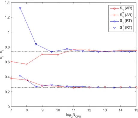
Fig. 2. Convergenceofnumericalestimatesof𝑆𝑥1and𝑆 𝑇

𝑥1fortheformulasusingRT(seeAppendix)withthosebasedontheacceptance-rejection(AR)approachfortheproductfunction

(39)definedinthetriangulardomainΩ1.

𝑝Ω₁ 2 (𝑥2|𝑥1)= 𝑝Ω1₍𝑥 1,𝑥2) 𝑝Ω1 1 (𝑥1) = 1 𝑥1. (42)

Expectation and total variance for this function can also be computed explicitly: 𝑓0=𝐸{𝑓(𝑥1,𝑥2)}=_∫ 1 0 ∫ 1 1−𝑥1 𝑥1𝑥22𝑑𝑥2𝑑𝑥1= 5 12, (43) 𝐷= ∫ 1 0 ∫ 1 1−𝑥1 (𝑥1𝑥2)22𝑑𝑥2𝑑𝑥1− (₅ 12 )2 = 3 80. (44)

Using the definition (7)of the main effect index in a non-rectangular area and the relationship between the main effect and total indices 𝑆𝑇

𝑥2=

1−𝑆_𝑥

1the sensitivity indices for the product function (39)are evaluated

as follows: 𝑆𝑥1= 1 𝐷 [ ∫1 0 𝑝 Ω1 1 (𝑥1)𝑑𝑥1 ( ∫1 1−𝑥1𝑓(𝑥1,𝑥2)𝑝 Ω1 2 (𝑥2|𝑥1)𝑑𝑥2 )2 −𝑓2 0 ] =80 3 [ ∫1 0 2𝑥1𝑑𝑥1 ( ∫1 1−𝑥1𝑥1𝑥2 1 𝑥1𝑑𝑥2 )2 −(5 12 )2] = 7 27 , (45) 𝑆𝑇 𝑥2=1−𝑆𝑥1= 20 27. (46)

Owing to the symmetry of the function and the area Ω1, 𝑆𝑥2=𝑆𝑥1

and 𝑆𝑇 𝑥1=𝑆

𝑇 𝑥2.

Note that in the absence of the constraint, i.e. when the variables are uniformly distributed in the unit square, the sensitivity indices are 𝑆𝑥1=𝑆𝑥2=3∕7 and 𝑆

𝑇 𝑥1=𝑆

𝑇

𝑥2=4∕7, while the mean value and total

variance are 𝑓0=1∕4 and 𝐷=7∕144.

We compare numerical performance of the formulas using RT and the acceptance-rejection (AR) approach. The details of the sampling scheme for RT is given in the Appendix. We recall that 𝑁CPU=𝑁(2𝑛+2) for RT while it is 𝑁CPU=𝑁(𝑛+2) for AR. From the convergence plots

Fig.2 it follows that the original formulas (4) and (5) with RT-based sampling (see Appendix) show efficiency similar to that of AR approach.

Fig. 3. DomainΩ2asdefinedbythelinearconstraint(48).

4.2. 2D g -function

In this Section we consider the so-called g-function which is often used in GSA for illustration purposes [1] in 2D:

𝑓= 2 ∏ 𝑖=1 ||4𝑥_𝑖−2||+𝑎_𝑖 1+𝑎_𝑖 (47)

with parameters 𝑎1=0 and 𝑎2=1 and ( x1, x2) uniformly distributed in the unit square. Below we compute its sensitivity indices when the feasible domain is restricted by a parametric linear Fig.3 or nonlinear Fig.9 constraint.

4.2.1. Alinearconstraint

In this subsection we consider a more general parametric linear con- straint (illustrated in Fig.3) than that used in the test case presented 223

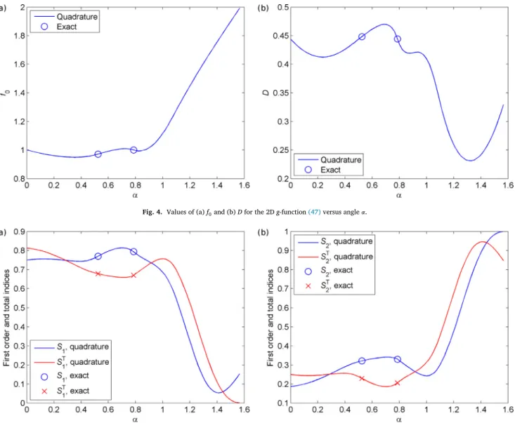
Fig. 4. Valuesof(a)f0and(b)Dforthe2Dg-function(47)versusangle𝛼.

Fig. 5. Valuesof(a)𝑆𝑥1and𝑆 𝑇

𝑥1,and(b)𝑆𝑥2and𝑆 𝑇

𝑥2forthe2Dg-function(47)versusangle𝛼.

Table 1

Exactvaluesofmean,totalvarianceandmaineffectsforselected valuesof𝛼. 𝛼 f0 D 𝑆𝑥1 𝑆𝑥2 0 1.0 4/9 3/4 3/16 𝜋/6 0.971413 0.448322 0.770349 0.321499 𝜋/4 1.0 4/9 −93 ₄₀ +₂ 9 ln2 −₂₀ 9 +9 ₈ ln2 𝜋/2 2.0 1/3 0.158883 1.0

in the previous subsection. The shape and size of the feasible domain

Ω₂are defined by the variable angle 𝛼between the top side of the unit square and the line defined by the linear constraint

𝑔(𝑥1,𝑥2)=1−tan(𝛼)𝑥1−𝑥2≥ 0. (48)

Firstly we obtain analytical results for two values of 𝛼:𝜋/6 and 𝜋/4. While the latter value leads to a symmetrical domain (complementary to Ω1considered in subsection4.1), the former does not result in any specific simplification of the problem. The reference values of the mean, total variance and main effects are given in Table1. Exact solution for 𝛼=𝜋∕6 was obtained using symbolic integration in Maple®, however the resulting expressions are too cumbersome to report them here, so the values are given in the decimal form to sufficient precision for error anal- ysis (see below). As noted above, the values of total sensitivity indices

are readily obtained from the relationships 𝑆𝑇

𝑥2=1−𝑆𝑥1, 𝑆 𝑇

𝑥1=1−𝑆𝑥2

which are valid in the 2D case.

Figs.4 and 5 show the variations of the expected value, total vari- ance and the main effect and total sensitivity indices with the angle 𝛼 changing from 0 to 𝜋/2, which corresponds to the whole range from the completely unconstrained 2D problem to the degenerate 1D case 𝑥1=0, x2∈ [0, 1]. Analytical exact values given in Table 1 are denoted by overlaid symbols. The results perfectly respect the limiting cases given in Table1. The numerical results were obtained with the use of the grid quadrature method.

As the value of 𝛼increases the levels of importance of the variables swap with x₁being initially significantly more important. However, as 𝛼→𝜋/2 the domain Ω2degenerates into the segment 𝑥1=0, 0 ≤x2 ≤ 1 so that the model function clearly ceases to depend on x1 explicitly however, it still depends on x₁implicitly via the constraint. This is re- flected by the value of the total effect index 𝑆𝑇

𝑥1dropping to zero as 𝛼→ 𝜋/2 and a simultaneous increase of 𝑆_𝑥2towards unity, while 𝑆𝑥1drops

to ∼0.054 before climbing back up again to 0.158883.

A comparison of the results obtained using QMC sampling employ- ing RT (see Appendix) and the acceptance-rejection method proposed herein is shown in Fig.6. It evidences that for the case of the 2D g- function the novel AR method converges to the analytical solution faster than that using RT in terms of the total number of model evaluations. Moreover, this is true for both first-order and total indices. Another ad-

Fig. 6. Convergenceofnumericalestimatesof𝑆𝑥1and𝑆 𝑇

𝑥1fortheoriginalformulasusingRTwiththosebasedontheacceptance-rejection(AR)approachforthe2Dg-function(47)for thecaseof𝛼=𝜋∕4.

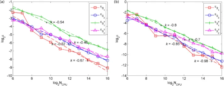
Fig. 7. RMSEconvergenceoftheMCestimatorsofSi(35)and𝑆𝑖𝑇(37)forthe2Dg-function(47)definedinΩ2for𝛼=𝜋∕6obtainedusing(a)MC(b)QMCmethods.

vantage of the AR approach is that it does not require the preliminary explicit evaluation of the relevant conditional cumulative distributions, which may be problematic even for feasible domains of simple shapes.

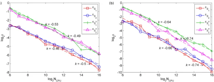
We also tested the performance of the different MC estimators. The root-mean-square error (RMSE) obtained using the MC estimator (35) for the main effect indices and the estimator (37) for total effects indices for a fixed value of 𝛼=𝜋∕6 is presented in Fig.7. To reduce the scatter in the error estimation the values of RMSE were averaged over L=50 independent runs: 𝜀𝑖= ⎛ ⎜ ⎜ ⎝ 1 𝐿 𝐿 ∑ 𝑙=1 ( 𝐼∗ 𝑖,𝑙−𝐼0 𝐼0 )2_⎞ ⎟ ⎟ ⎠ 1 2 . Here 𝐼∗

𝑖 is the numerical value of a particular estimator, I0 is the corresponding analytical value. The RMSE is approximated by a trend

line cNk_{. Values of kare given on the plots. The convergence rates of S} i and 𝑆𝑇

𝑖 for the MC method Fig.7(a) are close to theoretically expected value of 1/2. On the other hand, the convergence rates for the QMC method Fig.7(b) are significantly higher (not worse than 0.85 for the Siand 0.7 for 𝑆_𝑖𝑇). It should be noted that both approaches suffer from decreased convergence rates when the area of Ω2diminishes (data not shown) and the domain becomes elongated along the x₂axis. However, even in this case the QMC method still outperforms MC.

Finally, we compare the performance of the two presented estima- tors for the main effect indices: namely, the DLR (35) and the estimator (36)for the modified formula (8) by S. Kucherenko et al. [8], the latter is denoted as SK. The results presented in Fig.8 show significant ad- vantages of the DLR approach when considering the convergence rate versus the total number of sampling points N_CPU.

Fig. 8. RMSEconvergenceoftheDLR(35)andSK(36)MCestimatorsforSiforthe2Dg-function(47)definedinΩ2for𝛼=𝜋∕6using(a)MC(b)QMCmethods.

Fig. 9. Aseriesofparabolicconstraintsdefinedby(49)fordifferentvaluesof𝛽andthe contourlinesoftheg-function(47).

4.2.2. Aparabolicconstraint

In this subsection we consider a more complex example involving a nonlinear constraint of the form:

𝑔(𝑥1,𝑥2)=𝑥2−𝛽𝑥1

(

1−𝑥1

)

≥0, (49)

which describes the part of the unit square above a parabola Fig.9. Depending on the value of 𝛽the permissible domain is either connected ( 𝛽≤ 4) or disconnected ( 𝛽 >4) as illustrated in Fig.9. We note that the domain is non-convex for any value of 𝛽.

Variations of the function mean, total variance and main and to- tal effect sensitivity indices reveal highly nonlinear behavior shown in Figs.10and 11. The dashed lines in these Figs indicate the critical value 𝛽=4 for the connectedness of the feasible domain. It is also worth not- ing that the limits 𝛽→0 and 𝛽→∞represent the two extreme cases corresponding either to the unconstrained situation (unit square) or to the degenerate case when the feasible domain is the union of two dis- joint segments 𝑥1=0, 1,x2∈[0, 1], respectively. In the latter limit the numerical values of f₀, D, main and total effect sensitivity indices tend

toward the same limit as those under a linear constraint when 𝛼→𝜋/2 (compare with Figs.4 and 5).

Consider the particular case of 𝛽=4 which is the smallest value of 𝛽 when the feasible domain is essentially disconnected. The exact values for the mean, total variance and main effect indices are:

𝑓0 =3∕2, 𝐷= 521 1260− 4 35 √ 2, 𝑆𝑥1 = 3(384√2−575) 144√2−521 , 𝑆𝑥2 =− 3 2 264√2−293 144√2−521. (50)

Fig.12shows the variation of RMSE versus the total number of sam- pling points NCPUfor MC and QMC methods. The latter is clearly supe- rior to MC. 4.3. K-function K-function is defined as 𝐾= 𝑛 ∑ 𝑖=1 (−1)𝑖 𝑖 ∏ 𝑗=1𝑥𝑗, (51) where variables 𝑥𝑗, 𝑗=1,...,𝑛 are independent uniformly distributed random variables in [0, 1]. K-function is also used in GSA for illustration purposes (see f.e. [19]).

We consider four different cases for domain definitions. The first one is an unconstrained problem ( x∈Hn_{). In the other three cases the unit} hypercube is divided by a hyperplane into two parts one of which is the permissible region for the problem variables 𝑥𝑗, 𝑗=1,...,𝑛. All of these cases are considered in the four-dimensional space 𝑛=4. The constraints are as follows:

𝐼1∶𝑥1+𝑥2 ≤1, (52)

𝐼2∶𝑥3+𝑥4≤ 1, (53)

𝐼3∶𝑥1+𝑥3 ≤1. (54)

Fig. 10. Valuesof(a)f0and(b)Dforthe2Dg-function(47)versusparameter𝛽fromparabolicconstraint(49).

Fig. 11. Valuesof(a)𝑆𝑥1and𝑆 𝑇

𝑥1,and(b)𝑆𝑥2and𝑆 𝑇

𝑥2forthe2Dg-function(47)versusparameter𝛽fromparabolicconstraint(49).

Fig. 12. RMSEconvergenceoftheMCestimatesofSi(35)and𝑆𝑖𝑇(37)forthe2Dg-function(47)undertheparabolicconstraint(49)with𝛽=4obtainedusing(a)MC(b)QMCmethods.

Fig. 13. SchematicrepresentationofpermissibleregionsfortheK-function(shadedarea) inthe3Dcase.

See Fig.13 for a schematic plot illustrating I1constraint in the 3D space.

For the numerical estimation we make use of grid quadrature for- mulas (multidimensional trapezoidal rule) presented in Section3.2. In order to assess the accuracy of numerical computations in the uncon- strained case the exact solution for the total effect indices reported in [20]was used while the analytical solution for the main effect sensitivity indices was derived in this paper:

𝑆𝑖= (₁ 2 )2𝑖−2 +(−1 2 )𝑛+𝑖−2 +(1 2 )2𝑛 3 2− 3 5(−1)𝑛 ( 1 2 )𝑛−1 +₁₀1 ( 1 3 )𝑛−3 −3 ( 1 2 )2𝑛. (56)

For the situations involving the constraints (52)–(54)exact values of S_iand 𝑆𝑇

𝑖 were obtained with the aid of Maple® software.

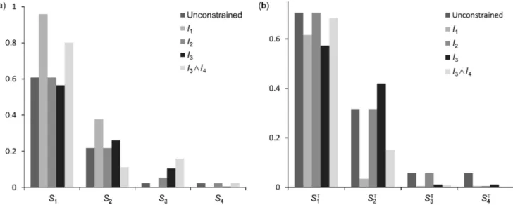
The exact values of Si and 𝑆_𝑖𝑇 for all four cases are presented in Fig.14. For the unconstrained case the most influential input is x1fol- lowed by x2with x3and x4having equal and much less significant con- tributions to the function variance.

Compared to the unconstrained case, the introduction of the first constraint defined by (52) (the indicator function I1) leads to a signif- icant increase of the main effect indices S₁and S₂accompanied by a simultaneous decrease of S3and S4. It reflects the fact that when the constraint (52)is imposed an even more substantial part of the variance is contributed by the first two terms of the K-function compared to the unconstrained case.

The second constraint (53)(the indicator function I2) introduces ad- ditional dependence between the less important variables x₃ and x₄.

Since x1and x2are not affected by I2their sensitivity indices (both main and total effects) remain at the same level as in the unconstrained case. However, variable x3features more prominently than x4compared with the unconstrained case although its value still remains small ( <0.1).

The third constraint (54) (the indicator function I₃) links an influ- ential variable x1and a significantly less important x3. It results in the decreased values of sensitivity indices of x1, while the values of sensitiv- ity indices of x2are increased. On the other hand, the main effect index of x3becomes significantly more important than in the unconstrained case drastically outrunning x4. However, the corresponding total effects

𝑆𝑇

3 and 𝑆𝑇4 turn out to be the same.

Finally, we consider a more general situation involving two inequal- ity constraints simultaneously: I3∩I4 (55). Each of the constraints in- volves an influential ( x1and x2, respectively) and a non-influential ( x3 and x₄, respectively) variable. The combination of these constraints has an effect on the total indices very similar to that from imposing a sin- gle constraint (52). This is not surprising given low importance of x3 and x₄and effective enhancement of 𝑆𝑇

1 through the structural inter- action of x1 with the other inputs Fig.14(b). On the other hand, al- though the first-order index S1is enhanced in comparison with the un- constrained problem as expected, the second most influential input in terms of total correlated contribution indices Siin this case turns out to be x3Fig.14(a) while x2drops to the third place. At the same time we notice that 𝑆₂𝑇 >𝑆₃𝑇. We recall Section2.4 that Sihas the meaning of total correlated contribution (full first-order sensitivity index) and 𝑆𝑇

𝑦 has the meaning of the total uncorrelated contribution (the independent total sensitivity index). Hence, the total uncorrelated contribution of x2 remains larger than that of x₃.

These examples based on the relatively simple K-function and ele- mentary constraints emphasize the strong and difficult-to-predict effects that constraining either model inputs or outputs may have on the rele- vant sensitivity indices.

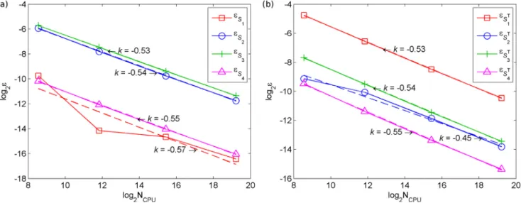
Fig. 15 shows the performance of the grid quadrature integra- tion method. Absolute errors of the estimates of S_i Fig.15(a) and 𝑆𝑇

𝑖

Fig.15(b) decrease in all cases at a rate 𝜀∼𝑂(𝑁−1∕2_{). This is indeed} as expected since the error of the trapezoidal rule (regardless of the dimensionality) is of the form ɛ ∼O( h2_{), where h is the grid spacing} assumed to be equal in all dimensions. Since the number of function evaluations in an n-dimensional space 𝑁∼ (1+1∕ℎ)𝑛(with equality in- stead of proportionality in the unconstrained case) we obtain that in general 𝜀∼𝑂(𝑁−2∕𝑛_).

Fig.16illustrates the performance of the MC estimators for DLR ap- proach for the main effect and the modified Sobol ’ formula for the total

Fig. 15. Relativeerrorin(a)Siandin(b)𝑆𝑖𝑇evaluatedusinggridquadratureversusthenumberoffunctionevaluationsNCPU,fortheK-functionunderconstraint(54)(definedbythe

indicatorI3).

Fig. 16. Convergenceratesofthe(a,b)DLRestimator(35)ofSiand(c,d)modifiedSobol’ estimator(37)of𝑆𝑖𝑇forthe4DK-functionunderconstraint(52)(definedbytheindicator

I1)obtainedusing(a,c)MCand(b,d)QMC.

Fig. 17. Projectionofthe10-dimentionalfeasibledomaindefinedby(58)ontothefirst threedimensions.

effect indices. Similarly to the previous examples, the use of QMC sam- pling results in faster convergence.

4.4. 10-dimensionalg-function

In this Section we consider a 10-dimensional g-function 𝑓= 10 ∏ 𝑖=1 ||4𝑥_𝑖−2||+𝑎_𝑖 1+𝑎_𝑖 (57)

with parameters 𝑎𝑖=[0,1,2,3,4,5,6,7,8,9]and 𝑥𝑖,𝑖=1,...,10uniformly distributed in the unit hypercube H10_{. Here we compute its sensitivity} indices when the feasible domain is restricted by

𝑔(𝑥1,...,𝑥10)=1−𝑓(𝑥1,...,𝑥10)≥0. (58) To illustrate the complexity of the resulting feasible domain we have plotted its projection onto the first three dimensions in Fig.17. It is ob- vious that the boundary of the domain defined by (58)cannot be readily described using explicit expressions. Moreover, (58)is an example of an output constraint, which cannot be evaluated independently from the

Table 2

Analytical(unconstrained case: GSA)andnumerical (con-strainedcase:cGSA)valuesofSiand𝑆𝑖𝑇.

i Si(GSA) Si(cGSA) 𝑆𝑖𝑇(GSA) 𝑆𝑇𝑖 (cGSA) 1 0.56066 0.68667 0.67050 0.95605 2 0.14017 0.00482 0.20631 0.19810 3 0.06230 0.00217 0.09579 0.10126 4 0.03504 0.00137 0.05473 0.06135 5 0.02243 0.00109 0.03529 0.04120 6 0.01557 0.00091 0.02461 0.02958 7 0.01144 0.00089 0.01812 0.02248 8 0.00876 0.00114 0.01390 0.01747 9 0.00692 0.00184 0.01100 0.01402 10 0.00561 0.00103 0.00891 0.01149

model function itself. In this particular case it can be interpreted as the introduction of an upper threshold for the model output f which affects all the inputs of the model.

The results of performing constrained GSA in this domain are pre- sented in Fig.18 and in Table2along with the analytical solutions for the unconstrained case [21]. It is notable that both the main and total effects of x1(the most influential input) increase upon the introduction of the constraint as a result of trimming off the parts of H10_{with signif-} icant variation due to the other inputs, and the presence of structural interactions with the other inputs. In line with this, the main indices of 𝑥𝑖,𝑖=2,...,10 decrease when the constraint is active. However, their total indices exceed those for the unconstrained case owing to the pres- ence of the structural dependences.

5. Conclusions

In this work, we have proposed a novel concept of constrained GSA which adds the ability to analyze model output variance in arbitrarily shaped n-dimensional domains. This amounts to greatly expanding the scope of GSA by allowing model variables to be subject to inequality constraints, which is common in a range of situations of practical im- portance.

The proposed formulas build upon Sobol ’ sensitivity indices and their recent development for models with dependent variables [8]. The ad- vantage of the presented formulations is that no prior knowledge of conditional or marginal distributions is assumed. All the required de- pendences are derived from the joint pdf in the presence of constraints. It is shown that the knowledge of the joint pdf corresponding to the un-