A novel power management and control design framework for resilient operation of microgrids

(1)

CRANFIELD UNIVERSITY

Mohammed H. Alkhafaji

A Novel Power Management and Control Design

Framework for Resilient Operation of Microgrids

School of Water, Energy, and Environment

Thesis Submitted for the Degree of

Doctor of Philosophy

Supervisors: Prof Patrick Chi-Kwong Luk

Dr John Economou

(2)

(3)

CRANFIELD UNIVERSITY

School of Water, Energy, and Environment

Thesis Submitted for the Degree of

Doctor of Philosophy

Mohammed H. Alkhafaji

A Novel Power Management and Control Design

Framework for Resilient Operation of Microgrids

Supervisors: Prof Patrick Chi-Kwong Luk

Dr John Economou

October 2017

© Cranfield University 2017. All rights reserved. No part of this

publication may be reproduced without the written permission of the

(4)

(5)

Abstract

This thesis concerns the investigation of the integration of the microgrid, a form of future electric grids, with renewable energy sources, and electric vehicles. It presents an innovative modular tri-level hierarchical management and control design framework for the future grid as a radical departure from the ‘centralised’ paradigm in conventional systems, by capturing and exploiting the unique characteristics of a host of new actors in the energy arena - renewable energy sources, storage systems and electric vehicles. The formulation of the tri-level hierarchical management and control design framework involves a new perspective on the problem description of the power management of EVs within a microgrid, with the consideration of, among others, the bi-directional energy flow between storage and renewable sources. The chronological structure of the tri-level hierarchical management operation facilitates a modular power management and control framework from three levels: Microgrid Operator (MGO), Charging Station Operator (CSO), and Electric Vehicle Operator (EVO). At

the top level is the MGO that handles long-term decisions of balancing the power flow between

the Distributed Generators (DGs) and the electrical demand for a restructure realistic microgrid model. Optimal scheduling operation of the DGs and EVs is used within the MGO to minimise the total combined operating and emission costs of a hybrid microgrid including the unit commitment strategy. The results have convincingly revealed that discharging EVs could reduce the total cost of the microgrid operation.

At the middle level is the CSO that manages medium-term decisions of centralising the

operation of aggregated EVs connected to the bus-bar of the microgrid. An energy management concept of charging or discharging the power of EVs in different situations includes the impacts of frequency and voltage deviation on the system, which is developed upon the MGO model above. Comprehensive case studies show that the EVs can act as a regulator of the microgrid, and can control their participating role by discharging active or reactive power in mitigating frequency and/or voltage deviations.

Finally, at the low level is the EVO that handles the short-term decisions of decentralising the

functioning of an EV and essential power interfacing circuitry, as well as the generation of low-level switching functions. EVO low-level is a novel Power and Energy Management System (PEMS), which is further structured into three modular, hierarchical processes: Energy Management Shell (EMS), Power Management Shell (PMS), and Power Electronic Shell (PES). The shells operate chronologically with a different object and a different period term. Controlling the power electronics interfacing circuitry is an essential part of the integration of EVs into the microgrid within the EMS. A modified, multi-level, H-bridge cascade inverter without the use of a main (bulky) inductor is proposed to achieve good performance, high power density, and high efficiency. The proposed inverter can operate with multiple energy resources connected in series to create a synergized energy system. In addition, the integration of EVs into a simulated microgrid environment via a modified multi-level architecture with a novel method of Space Vector Modulation (SVM) by the PES is implemented and validated experimentally. The results from the SVM implementation demonstrate a viable alternative switching scheme for high-performance inverters in EV applications.

The comprehensive simulation results from the MGO and CSO models, together with the experimental results at the EVO level, not only validate the distinctive functionality of each layer within a novel synergy to harness multiple energy resources, but also serve to provide compelling evidence for the potential of the proposed energy management and control framework in the design of future electric grids. The design framework provides an essential design to for grid modernisation

(6)

(7)

Acknowledgments

All Praise to our almighty GOD, Lord of the worlds, for all his blessings and among them enabling me to complete this thesis.

The research journey would not have been as interesting without the fascinating people I met along the way.

I would like to express my deepest gratitude to my first supervisor Prof Patrick Luk for the opportunity to carry out this research project. The patience, support, encouragement, and the useful advice that he has provided throughout the project is very much appreciated.

I would like to express the deepest gratitude to my second supervisor Dr John Economou for his valuable comments and useful discussions. I am most grateful for the encouragement and support that he gave me in writing my thesis.

I would also like to express my sincere gratitude to Dr Maciej Bendyk who helps me to do a ‘proper-job’ calibre, Dr Akram Bati, Dr Mutaz Shunasi for their valuable assistance, and Prof Philip Longhurst for his insightful recommendations and valuable assistance.

A special thank you goes out to Sam Skears and Heather Simpkins for the perfect understandable, hard activate and nice treatment that they offer to me. I am most grateful for the extensive support Sam gave me along the way of the study and the useful correction Heather gave me in writing my thesis.

I would also express my deepest gratitude to viva examiners: Prof Jun Liang, Dr James Whidborne, and Dr Mark Pawlett for awarded me the PhD degree with useful advices and corrections.

I gratefully acknowledge the financial support of my PhD study from the Iraqi Ministry of Higher Education and Scientific Research (MOHESR) in Baghdad and Cultural Attaché in London. My sincere thanks are forwarded to my colleagues at Cranfield University for their support, cooperation, and friendly company.

I would also express special thanks to Alison Digger, Joanne Holden, and Chris Binch for teaching, encouraging, and supporting me through the English language course program at Cranfield University.

My sincere appreciation for the tremendous support provided by Cranfield University’s technical staff, accommodation office’s staff, library’s staff, Information department’s staff, and all workshop’s staff.

My heartfelt appreciation goes out to my precious parents, parents-in-law, my brother (Ali), brothers-in-law, and sister-in-law, my gorgeous daughters for their love, encouragement, and unfailing support.

I owe the greatest debt of gratitude to my Mum and my Dad for their love, patience, support, sacrifice, teaching me the art of transforming imagination into something real, and never forget supplicate to me. I am an extension of both, and proud of it.

Finally,

To my beloved wife, Iman, for tolerating my eccentric ways the past ten years, giving me three lovely kids, and for agreeing to stand by me forever.

(8)

(9)

List of Figures

Figure 1-1: Applicability of Pathways based on Present Status of Power Sector Organization

[2] ... 2

Figure 1-2: Electrical power transmission and distribution losses of various countries in percentage of output for 2013 [7] ... 2

Figure 1-3: Annual worldwide percentage losses[7] ... 3

Figure 1-4: Global greenhouse gas emissions by Economic Sector [15] ... 3

Figure 1-5: World electricity production from all energy sources in 2014 [16] ... 4

Figure 1-6 Estimated Renewable Energy Share of Global Final Energy Consumption, 2014 [1] ... 6

Figure 1-7: Greenhouse gas emissions by sector in UK during Q1 and Q2 of 2016 [56] ... 10

Figure 1-8: Evaluation of the global electric car stock, 2010-2015 [57] ... 11

Figure 1-9: Evolution of battery energy density and cost [57] ... 11

Figure 1-10: Microgrid network architecture ... 17

Figure 1-11: Research methodology ... 20

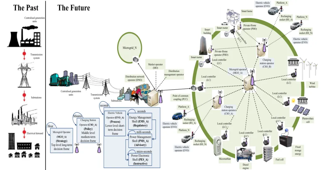
Figure 1-12: The general structure of the conventional power system and the smart grid system ... 24

Figure 1-13: Hierarchical and decision timeframes of management model ... 25

Figure 1-14: Concept of a modular management structure ... 27

Figure 1-15: Outline of the thesis structure ... 35

Figure 1-16 Thesis’ Structure, Aim and objectives, Tasks, and Novelties ... 36

Figure 2-1: Shares of UK greenhouse gas emissions in 2014 [73] ... 40

Figure 2-2: Shares of UK electricity generation in 2014 [73] ... 40

Figure 2-3: The first Electric vehicle model by Ányos Jedlik in 1828. ... 41

Figure 2-4: The first Electric motor model by Ányos Jedlik in 1827. ... 41

Figure 2-5: Publication on electric vehicle and microgrid extracted from Scopus database ... 41

Figure 2-6: Smart grid structure [88] ... 43

Figure 2-7: The centralised controller levels ... 48

Figure 2-8: Typical microgrid structure ... 51

Figure 2-9: EV management structure ... 55

Figure 2-10: Electric vehicle connection platform ... 56

Figure 2-11: Bi-directional power flow ... 57

Figure 2-12: Bi-directional topology ... 58

Figure 2-13: Three-phase H-bridge cascade multi-level convert ... 60

Figure 2-14: General dynamics of a model and their relationships ... 62

Figure 2-15: Two level rotating reference vector switching states of SVPWM ... 64

Figure 2-16: Two level carrier based SPWM [239] ... 65

Figure 2-17: Carriers based linear regulation control method ... 66

Figure 2-18: Hysteresis control method (Bang-Bang control strategy) ... 66

Figure 2-19: Peak current control method ... 67

Figure 2-20: Proportional resonant current control method ... 67

Figure 2-21: Vector transformations ... 68

(18)

Figure 2-23: Rotating reference frame control method ... 69

Figure 2-24: Idealised three phase synchronous generator [256] ... 71

Figure 2-25: Synchronverter control scheme ... 72

Figure 2-26: Scalar control scheme ... 73

Figure 2-27: Vector control scheme ... 74

Figure 2-28: Transmission line power flow ... 75

Figure 2-29: Droop characteristic for generator ... 76

Figure 2-30: Passive hybrid topology ... 76

Figure 2-31: Parallel semi-active hybrid topology ... 76

Figure 2-32: Capacitor semi-active hybrid topology ... 77

Figure 2-33: Battery semi-active hybrid topology ... 77

Figure 2-34: Series active hybrid topology ... 77

Figure 2-35: Parallel Active Hybrid topology ... 78

Figure 3-1: Flow chart diagram explaining the voltage stability identification. ... 83

Figure 3-2: Flow charts of the DG placement algorithms ... 86

Figure 3-3: Case study ... 88

Figure 3-4: Voltage profile for the conventional grid (without DG impact) ... 89

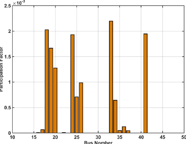
Figure 3-5: Participation factor for the conventional grid (without DG impact) ... 89

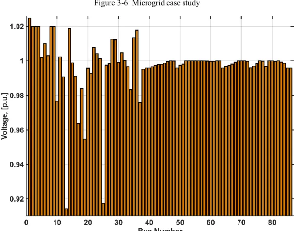
Figure 3-6: Microgrid case study ... 91

Figure 3-7: Voltage profile for the smart grid at connected mode (with DG impact) ... 91

Figure 3-8: Participation factor for the smart grid at connected mode (with DG impact) ... 92

Figure 3-9: Voltage profile for smart grid at isolated mode ... 92

Figure 3-10: Participation factor for smart grid at isolated mode ... 93

Figure 3-11: Voltage profile for microgrid at isolated mode ... 93

Figure 3-12: Participation factor for microgrid at isolated mode ... 94

Figure 3-13: Voltage profile comparison of transmission system for all scenarios ... 95

Figure 3-14: Voltage profile comparison of distribution network for all scenarios ... 95

Figure 3-15: Voltage profile comparison for all scenarios ... 96

Figure 3-16: Critical load angle against range of capacitor shunt compensation ... 101

Figure 3-17: Critical voltage at receiving end bus against range of capacitor shunt compensation ... 101

Figure 3-18: Critical power at receiving end voltage against range of capacitor shunt compensation ... 102

Figure 3-19: Surge impedance loading against range of capacitor shunt compensation ... 102

Figure 3-20: Voltage profile for microgrid at isolated mode and isolating the generator of bus bar 45 ... 103

Figure 3-21: Participation factor for microgrid at isolated mode and isolating the generator of bus bar 45 ... 104

Figure 3-22: Voltage profile for system with ten EV compensation at weakest bus 25 ... 104

Figure 3-23: Voltage profile for system with ten EV compensation at minimum voltage bus 46 ... 105

Figure 3-24: Voltage profile for system with ten EV compensation at bus 25 & 46 ... 105

Figure 3-25: Participation factor for system with ten EV compensation at bus 25 ... 106

(19)

Figure 3-27: Participation factor for system with ten EV compensation at bus 25 & 46 ... 107

Figure 3-28: Voltage profile comparison of microgrid at different connected EVs buses ... 108

Figure 4-1: The optimisation algorithm ... 113

Figure 4-2: Flow chart of microgrid optimisation strategy ... 114

Figure 4-3: The input solar irradiation to the model (Experimental data with linear interpolations) [286]... 115

Figure 4-4: The input temperature to the model (Experimental data with linear interpolations) [286] ... 115

Figure 4-5: The input wind speed to the model (Experimental data with linear interpolations) [286] ... 116

Figure 4-6: Wind turbine power generation (simulated results) ... 118

Figure 4-7: Photovoltaic model ... 119

Figure 4-8: Photovoltaic power generation (simulated results) ... 120

Figure 4-9: Daily load curve (Experimental Data with Linear Interpolation) [19] ... 131

Figure 4-10: Type and efficiency of distributed generator [306] ... 132

Figure 4-11: Proposed Utility Grid Tariff ... 133

Figure 4-12: Hourly optimal power schedule of DGs under isolated mode with UC consideration (Simulated results). ... 135

Figure 4-13: Hourly total DGs operating cost under isolated mode with UC consideration (Simulated results). ... 136

Figure 4-14: Hourly optimal power schedule of DGs under isolated mode without UC consideration (Simulated results). ... 137

Figure 4-15: Hourly total DGs operating cost under isolated mode without UC consideration (Simulated results) ... 138

Figure 4-16: Hourly optimal power schedule of DGs and exchange power with UG under grid connected mode with UC consideration and pollutant treatment consideration (Simulated results). ... 140

Figure 4-17: Hourly total DGs operating cost under grid connected mode with UC consideration and emission consideration (Simulated results). ... 141

Figure 4-18: Hourly optimal power schedule of DGs and exchange power with UG under grid connected mode without UC consideration and emission consideration (Simulated results). ... 142

Figure 4-19: Hourly total DGs operating cost under grid connected mode without UC consideration and emission consideration (Simulated results) ... 142

Figure 5-1: CSO optimisation algorithm ... 147

Figure 5-2: Flow chart of CSO optimisation algorithm ... 148

Figure 5-3: Electric vehicles’ smart charger architecture ... 150

Figure 5-4: Information of EVA to CSA of each EV at connected time ... 152

Figure 5-5: Schematic diagram of connected electric vehicles to microgrid ... 153

Figure 5-6: Schematic diagram of CSO ... 154

Figure 5-7: CSO infrastructure ... 154

Figure 5-8: Charging schedule factor of battery and supercapacitor ... 158

Figure 5-9: Discharging schedule factor of battery ... 158

(20)

Figure 5-11: Explanation of applied scenarios ... 163

Figure 5-12: SoC of charging EVs with power demand 100% ... 167

Figure 5-13: Power consumed of charging EVs with power demand 100% ... 167

Figure 5-14: Number of vehicles connected vs. number of vehicles that do not achieve the desired SoC at a specific time ... 168

Figure 5-15: Number of vehicles connected vs. number of vehicles that do charge at a specific time ... 168

Figure 5-16: The cost of power charging for each vehicle ... 169

Figure 5-17: SoC from charging EVs with power demand 100% ... 173

Figure 5-18: Power consumed from charging EVs with power demand 100% ... 173

Figure 5-20: Number of vehicles connected vs. number of vehicles not charging at a specific time ... 174

Figure 5-22: SoC of charging EVs with power demand at 75%... 179

Figure 5-23: Power consumed of charging EVs with power demand at 75% ... 179

Figure 5-24: The state of charge of each vehicle at departure time at the optimisation function ... 180

Figure 5-25: The state of charge of each vehicle at departure time after applying the priority strategy ... 180

Figure 5-26: Number of EVs connected vs. number of EVs that do not achieve the desired SoC ... 180

Figure 5-27: Number of vehicles connected vs. number of vehicles do charge at time ... 181

Figure 5-28: The total charging cost of each vehicle at the optimisation function... 181

Figure 5-29: The total charging cost of each vehicle after applying the priority strategy ... 182

Figure 5-30: SoC of charging EVs with power demand ... 186

Figure 5-31: Power consumed of charging EVs with power demand ... 186

Figure 5-32: The state of charge of each vehicle at departure time ... 187

Figure 5-34: Number of vehicles connected vs. number of vehicles do charge at specific time ... 188

Figure 5-35: The cost of power charging of each vehicle ... 188

Figure 5-36: Cost compression for all cases ... 190

Figure 5-37: SoC of each vehicle along connected time ... 195

Figure 5-38: Power of each vehicle along connected time ... 195

Figure 6-1: EVO optimisation algorithm ... 201

Figure 6-2: Battery basic equivalent circuit and voltage characteristic ... 203

Figure 6-3: Combined method for practical implementation of SoC estimation (adapted from [324, Sec. 3.12], [327, Sec. 7.2.1]) ... 206

Figure 6-4: Modelling of supercapacitor ... 207

(21)

Figure 6-6: The capability of the power delivery of the battery and supercapacitor for a small

vehicle based on NYCC driving cycle. ... 211

Figure 6-7: Bidirectional converter topology ... 212

Figure 6-8: Voltage ripple due to inductor ... 213

Figure 6-9: Voltage ripple due to capacitor ... 213

Figure 6-10: Voltage ripple due to both inductor and capacitor ... 213

Figure 6-11: Evolution of the output voltage of a buck–boost converter with the duty cycle when the parasitic resistance of the inductor increases [337]. ... 214

Figure 6-12: Closed loop controller ... 215

Figure 6-13: Schematic diagram of a modified H-bridge multi-level converter ... 216

Figure 6-14: Block diagram to detect the fundamental voltage positive sequence. ... 222

Figure 6-15: Block diagram of the PLL circuit [350, p. 142] ... 222

Figure 6-16: (a) Represents power flow through a line. (b) Represents the phasors diagram ... 222

Figure 6-17: Frequency and voltage droop characteristics ... 224

Figure 6-18: Schematic diagram of droop controller ... 227

Figure 6-19: Voltage restoration ... 227

Figure 6-20: Frequency restoration ... 227

Figure 6-21: Vector controller ... 229

Figure 6-22: PMS fuzzy inference system block diagram ... 232

Figure 6-23: Fuzzy rule of battery reference at Vm = 227V and SoCsc = 50% ... 232

Figure 6-24: Fuzzy rule of battery reference at Vm = 205V and SoCsc = 50% ... 232

Figure 6-25: Fuzzy rule of battery reference at Vm = 194 and SoCsc = 50% ... 233

Figure 6-26: Fuzzy rule of supercapacitor reference at Fm = 50Hz and SoCb = 75% ... 233

Figure 6-27: Fuzzy rule of supercapacitor reference at Fm = 49.85Hz and SoCb = 75% ... 233

Figure 6-28: Fuzzy rule of supercapacitor reference at Fm = 49.7Hz and SoCb = 75% ... 233

Figure 6-29: Fuzzy Sugeno input membership functions’ plots of frequency... 233

Figure 6-30: Fuzzy Sugeno input membership functions’ plots of voltage ... 233

Figure 6-31: Fuzzy Sugeno input membership functions’ plots of SoCb ... 234

Figure 6-32: Fuzzy Sugeno input membership functions plots’ of SoCsc ... 234

Figure 6-33: Fuzzy Sugeno output weight functions’ plots of battery reference ... 234

Figure 6-34: Fuzzy Sugeno output weight functions’ plots of supercapacitor reference ... 234

Figure 6-35: Switching state for the first sextant ... 237

Figure 6-36: Triangle coordinate ... 239

Figure 6-37: The region number according to 𝑘1, 𝑘2, 𝑘3 ... 239

Figure 6-38: Overmodulation of SVPWM method ... 242

Figure 6-39: Flow chart space vector pulse width modulation algorithm ... 244

Figure 6-40: Line voltage waveforms of inverter (simulated results) ... 245

Figure 6-41: Line voltage waveforms of inverter (experimental results) ... 245

Figure 6-42: Line voltage waveforms of three-phase bridge (simulated results) ... 246

Figure 6-43: Line voltage waveforms of three-phase bridge (experimental results) ... 246

Figure 6-44: Line voltage waveforms of H-bridge (simulated results) ... 247

Figure 6-45: Line voltage waveforms of H-bridge (experimental results) ... 247

(22)

Figure 6-47: Phase voltage waveforms of Inverter (experimental results) ... 248 Figure 6-48: Phase voltage waveforms of three-phase bridge (simulated results) ... 249 Figure 6-49: Phase voltage waveforms of three-phase Bridge (experimental results) ... 249 Figure 6-50: Phase voltage waveforms of H-bridge (simulated results) ... 250 Figure 6-51: Phase voltage waveforms of H-bridge (experimental results) ... 250 Figure 6-52: Standard three-leg inverter hexagon diagram ... 252 Figure 6-53: Modified H-bridge multi-level inverter at battery charging mode. ... 252 Figure 6-54: States of charge, current, and voltage waveforms of battery (simulated results) ... 253 Figure 6-55: Battery, supercapacitor, and inverter current waveforms (simulated results) ... 254 Figure 6-56: Modified H-bridge multi-level inverter at supercapacitors charging mode (the semiconductor switches). ... 256 Figure 6-57: H-bridge hexagon diagram... 256 Figure 6-58: State of charge, current, and voltage waveforms of supercapacitor connected at phase A (simulated results) ... 257 Figure 6-59: Battery, supercapacitor, and inverter current waveforms at supercapacitors charging mode (simulated results) ... 258 Figure 6-60: Balance current waveforms of supercapacitors (simulated results) ... 259 Figure 6-61: Unbalanced current waveforms of supercapacitors (simulated results) ... 259 Figure 6-62: Hexagon diagram of modified H-bridge multi-level inverter. ... 261 Figure 6-63: States of charge current and voltage waveforms of battery (simulated results) 262 Figure 6-64: States of charge, current, and voltage of supercapacitor at discharging mode (simulated results) ... 263 Figure 6-65: Battery, supercapacitor, and inverter current waveforms (simulated results) ... 264 Figure 6-66: Battery, supercapacitor, and inverter voltage waveforms (simulated results) .. 265 Figure 6-67: Three-phase currents and voltages of the inverter (simulated results) ... 266 Figure 6-68: Active power of inverter, battery, and supercapacitor of EV at different ranges of injection of active power to the microgrid (simulated results) ... 268 Figure 6-69: Reactive power of inverter, battery, and supercapacitor of EV at different ranges of injection of reactive power to the microgrid (simulated results) ... 268 Figure 6-70: Active power of inverter, battery, and supercapacitor of EV at different ranges of injection of active and reactive power to the microgrid (simulated results) ... 269 Figure 6-71: Reactive power of inverter, battery, and supercapacitor of EV at different ranges of injection of active and reactive power to the microgrid (simulated results) ... 269 Figure 7-1: Overall layout of experimental rig ... 275 Figure 7-2: Inverter overview ... 275 Figure 7-3: Rig overview ... 276 Figure 7-4: Architecture of the CompactRIO system ... 277 Figure 7-5: Waveforms of the three-phase bridge at output voltage 40 V ... 283 Figure 7-6: Waveforms of three-phase bridge at output voltage 50 V ... 283 Figure 7-7: Waveforms of three-phase bridge at output voltage 60 V ... 284 Figure 7-8: Waveforms of three-phase bridge at output voltage 65 V ... 284 Figure 7-9: Waveforms of H-Bridge at output voltage 40 V ... 285 Figure 7-10: Waveforms of H-Bridge at output voltage 50 V ... 285

(23)

Figure 7-11: Waveforms of H-Bridge at output voltage 60 V ... 286 Figure 7-12: Waveforms of H-Bridge at output voltage 65 V ... 286 Figure 7-13: Waveforms of Inverter at output voltage 40 V ... 287 Figure 7-14: Waveforms of Inverter at output voltage 50 V ... 287 Figure 7-15: Waveforms of Inverter at output voltage 60 V ... 288 Figure 7-16: Waveforms of Inverter at output voltage 70 V ... 288 Figure 7-17: Waveforms of Inverter at output voltage 80 V ... 289 Figure 7-18: Waveforms of Inverter at output voltage 90 V ... 289 Figure 7-19: Waveforms of Inverter at output voltage 100 V ... 290 Figure 7-20: Waveforms of Inverter at output voltage 110 V ... 290 Figure 7-21: Waveforms of Inverter at output voltage 120 V ... 291 Figure 7-22: Waveforms of Inverter at output voltage 128 V ... 291 Figure 7-23: Phase waveforms of three-phase bridge at output voltage 40 V ... 292 Figure 7-24: Phase waveforms of three-phase bridge at output voltage 50 V ... 292 Figure 7-25: Phase waveforms of three-phase bridge at output voltage 60 V ... 293 Figure 7-26: Phase waveforms of three-phase bridge at output voltage 65 V ... 293 Figure 7-27: Phase waveforms of H-bridge at output voltage 40 V ... 294 Figure 7-28: Phase waveforms of H-bridge at output voltage 50 V ... 294 Figure 7-29: Phase waveforms of H-bridge at output voltage 60 V ... 295 Figure 7-30: Phase waveforms of H-bridge at output voltage 65 V ... 295 Figure 7-31: Phase waveforms of Inverter at output voltage 40 V ... 296 Figure 7-32: Phase waveforms of Inverter at output voltage 50 V ... 296 Figure 7-33: Phase waveforms of Inverter at output voltage 60 V ... 297 Figure 7-34: Phase waveforms of Inverter at output voltage 70 V ... 297 Figure 7-35: Phase waveforms of Inverter at output voltage 80 V ... 298 Figure 7-36: Phase waveforms of Inverter at output voltage 90 V ... 298 Figure 7-37: Phase waveforms of Inverter at output voltage 100 V ... 299 Figure 7-38: Phase waveforms of Inverter at output voltage 110 V ... 299 Figure 7-39: Phase waveforms of Inverter at output voltage 120 V ... 300 Figure 7-40: Phase waveforms of Inverter at output voltage 128 V ... 300

List of Figures

in

Appendices

Apx_Figure D-1: Schematic diagram of the equivalent π model with load ... 343 Apx_Figure E-1: Schematic diagram of the equivalent π model with source ... 344 Apx_Figure F-1: Equivalent π model for long length line ... 345 Apx_Figure H-1: Schematic diagram of inverter topology ... 346 Apx_Figure K-1: CompactRIO cRIO-9012 configuration[353] ... 356 Apx_Figure K-2: CRIO chassis connection to CRIO controller ... 356 Apx_Figure K-3: NI 9425 model configuration ... 357 Apx_Figure K-4: NI 9476 model configuration ... 357 Apx_Figure K-5: NI 9474 model configuration ... 357 Apx_Figure K-6: NI 9402 model configuration ... 357

(24)

Apx_Figure K-7: NI 9201 model configuration ... 358 Apx_Figure K-8: Schematic diagram of Modified Cascade Multi-Level Inverter (MCMLI) with gate drive [Extended design of [353]] ... 358 Apx_Figure K-9: Schematic diagram of gate drive circuit [Extended design of [353]] ... 359 Apx_Figure K-10: Schematic diagram of Modified Cascade Multi-Level Inverter (MCMLI) [Extended design of [353]] ... 359 Apx_Figure K-11: Schematic diagram of digital optoisolator [Extended design of [353]] .. 360 Apx_Figure K-12: Schematic diagram of analogue optoisolator [Extended design of [353]] ... 360 Apx_Figure K-13: Schematic diagram of voltage measurement interface [Extended design of [353]]... 361 Apx_Figure K-14: Schematic diagram of MCMLI including voltage and current sensing [Extended design of [353]] ... 361 Apx_Figure K-15: Schematic diagram of battery bank and supercapacitor bank [Extended design of [353]] ... 362 Apx_Figure K-16: Schematic diagram of input LC_filter for induction motor [Extended design of [353]] ... 362 Apx_Figure L-1: MATLAB print screen programming ... 365 Apx_Figure L-2: Lab VIEW print screen programming [Extended design of [353]] ... 369

(25)

List of Tables

Table 1-1: Battery capacity of different types of Electric Vehicle ... 13 Table 2-1: The distributed generator classification ... 46 Table 3-1: Distributed generator arrangement on buses ... 85 Table 3-2: The eigenvalue for lowest buses ... 85 Table 3-3: EVs connection detail ... 103 Table 4-1: Distributed generators compression [297]–[300] ... 121 Table 4-2: The criteria of the judgment matrix ... 125 Table 4-3: Distributed generators’ type, range, and location ... 132 Table 4-4: Parameter constant of the grid equipment [104], [287], [288], [302], [303], [305]. ... 132 Table 4-5: Daily cost of total DGs operating cost under isolated mode with UC consideration ... 136 Table 4-6: Daily cost of total DGs operating cost under isolated mode without UC consideration ... 138 Table 4-7: Daily cost of total DGs’ operating cost under grid connected mode with UC consideration ... 140 Table 4-8: Daily cost of total DGs’ operating cost under grid connected mode without UC consideration ... 141 Table 5-1: Typical characteristics of different charging modes as defined by the IEC [319]. ... 151 Table 5-2: Frequency and voltage range of operation ... 156 Table 5-3: Map range of frequency and voltage deviation ... 157 Table 6-1: Performance comparison between supercapacitor and Lithium-ion [331]. ... 208 Table 6-2: Parameters for a typical small EV. ... 210 Table 6-3: Standard three-leg inverter generation pattern ... 218 Table 6-4: H-bridge generation pattern... 219 Table 6-5: Switching state ... 236 Table 6-6: Example ... 239 Table 7-1: Induction motor parameter ... 274

List of Tables in Appendices

Apx_Table I-1: Distributed generators operation at unit commitment consideration of isolated mode optimisation including operation and pollutants treatment policy ... 350 Apx_Table I-2: Distributed generators operation at unit commitment consideration of connected mode optimisation including operation and pollutants treatment policy ... 350 Apx_Table J-1: Input data of case study... 352

(26)

(27)

List of Abbreviations

AC Alternating current

CPS Conventional power system

CSA Charging station agency

CSC Centralised smart charging

CSO Charging station operator

CSS Charging station system

DC Direct current

DG Distributed generator

DNO Distribution network operator

DSC Decentrlised smart charging

EMS Energy management shell

EVA Electric vehicle agency

EVO Electric vehicle operator

EVs Electric vehicles

ICE Internal composition engine

MGO Microgrid operator

MIQP Mixed integer quadratic programming

MILP Mixed integer linear programming

PES Power electronic shell

PF Participation factor

PMS Power management shell

RS Recharging socket

RSA Recharging socket agency

SCA Smart controller agent

(28)

(29)

Nomenclature

Latin Symbols

A,B,C,D Generalized circuit constant

𝐴0, 𝐵0 Generalised line constant

𝐶_𝑑 Degradation cost

𝐶𝐹(𝑃_𝑖) Operating cost of the generating unit 𝑖 in $/h

𝐶𝑖 Fuel costs of the generating unit 𝑖 in $/𝑙 for DE and $/𝑘𝑊ℎ for FC and

MT

𝐶𝑘 Treatment cost of the 𝐾𝑡ℎ type of pollutants emission in $/kg

𝐶_𝑛𝑙 Natural gas price to supply the Microturbine

𝐶𝑟𝑎𝑡𝑒,𝑝𝑐ℎ/𝑞𝑐ℎ General active power and reactive power price of charging electricity

respectively, for example charging rate is 0.08$/kWh.

𝐶_{𝑟𝑎𝑡𝑒,𝑝𝑑𝑖𝑠/𝑞𝑑𝑖𝑠} General active power and reactive power price of discharging electricity

respectively, for example, discharging rate is 1.2$/kWh.

D Duty cycle

𝐷 Binary number of the owner choice for either bi-directional power or

unidirectional one.

𝐷 Daily electricity demand

𝐸_𝑏(𝑡) State of charge of the battery at the current state.

𝐸_𝑏(𝑡 − 1) State of charge of the battery at the previous state.

𝐸_𝑗𝑟𝑒𝑞𝑢𝑖𝑟𝑒𝑑 Battery capacity of the jth electric vehicle

𝐸_𝑛 Energy produced by a generator 𝑛

𝐸𝑝𝑣 Photovoltaic energy produced

𝐹 Difference in charging and discharging rate for example charging rate 1

$/kWh from 00-8 am, 1.2 $/kWh from 8-16, and 1.1 $/kWh from15-00.

𝐹𝑖 Fuel consumption rate of a generating unit 𝑖

𝐹(𝑃𝑖) Operating cost of the generating unit 𝑖 in $/h

𝐾 Scale factor to normalise vector ∆𝑄

𝐺 Solar irradiation in (W/m3_).

𝐺𝑑 Average daily solar radiation value.

𝐼 Model current (Ampere).

𝐼₀ Saturation current of the diode

I_L Dc load current

𝐼𝐿 Light generated current.

𝐼_𝑜𝑟 Cell saturation current at 𝑇𝑟

𝐼_𝑜𝑠 Cell reverse saturation current.

𝐼𝑆𝐶𝑅 Short circuit current at 25oC and 1000W/m2

𝐽 Jacobian matrix

𝐽_𝑅 Reducible Jacobian matrix

(30)

𝐾_𝐼 Short circuit current temperature coefficient at 𝐼𝑆𝐶𝑅𝐾𝐼 = 0.0035𝐴/𝑜𝐶

𝐾_{𝑓.𝑐ℎ/𝑑𝑖𝑠} Charging or discharging factor from log function of SoC

𝐾_𝑜𝑚 Proportional maintenance constant of unit 𝑖

𝑀 logical number i for grid connected and 0 for grid disconnected

𝑁 Total number of the DG in the microgrid

𝑂𝑀𝑖 Operating and maintenance cost of a generating unit 𝑖 in $/h

𝑃_𝐺2𝑉 Net power capacity available to recharge EVs in G2V mode.

P₀ Set point of active power

𝑃_𝐽 Electric power introduces at interval 𝐽

𝑃𝑉2𝐺 Aggregated power flow from EVs to grid in V2G mode

𝑃_{𝑉2𝐺,𝑚𝑎𝑥} Maximum allowed power at 𝑖𝑡ℎ EVs sources can be discharged.

𝑃_{𝑐ℎ\𝑑𝑖𝑠,𝑖𝑗} Power of charging or discharging in a time i for electric vehicle j which is

Control variable of the objective function

𝑃_{𝑐𝑠,𝑑𝑖𝑠} Power of discharging charging station

𝑃_𝑑 Power demand from non-electric vehicle load

𝑃_{𝑑𝑔,𝑖} Diesel generator (i) output power (kW)

𝑃_{𝑔𝑟𝑖𝑑} Output power of the grid

𝑃_𝑖 Decision variables that are representing the real power output from

generating unit 𝑖 in kW.

𝑃_𝑖 Output power of an ith distributed generator

𝑃_𝑗,𝑏𝑎 Active power required from MGO

𝑃_𝑗,𝑏𝑟 Battery rated charging power used to charge jth electric vehicle during the

interval t

𝑃_{𝑗,𝑠𝑐}𝑟 Supercapacitor rated charging power used to charge jth electric vehicle

during the interval t

𝑃𝑚𝑖𝑛, 𝑃𝑚𝑎𝑥 Minimum power and maximum power for charging station that provides

from MGO in charging mode or by the state of the electric vehicle in the discharging mode.

𝑃_𝑛 Daily resource energy

𝑃_𝑛𝑒𝑡 = 𝑃_𝑠− 𝑃_𝑑 Net power capacity available

Pr Real power

𝑃_𝑠 Scheduled power

Q₀ Set point of reactive power

𝑄_𝑗 Rated ampere hour rating (AHR) of the jth battery

𝑄_𝑗,𝑏𝑎 Reactive power required from MGO

Q_r Reactive power

𝑅_𝑛 Rated power of the generators

𝑅_𝑠 Series resistance (ohm).

𝑅𝑠ℎ Shunt resistance (ohm).

𝑆𝐶_𝑖 Start-up cost of a generating unit 𝑖 in $/h

𝑆𝑜𝐶_𝐵𝑎 Actual state of charge

(31)

𝑆𝑜𝐶_{𝑏\𝑠𝑐,𝑖𝑗}𝑑 State of charge of battery or supercapacitor at departure time

𝑆𝑜𝐶_{𝑏\𝑠𝑐,𝑖𝑗} State of charge for either battery or supercapacitor in time I for electric

vehicle j.

𝑆𝑜𝐶_𝑚𝑎𝑥 Upper limits of the state of charge.

𝑆𝑜𝐶_𝑚𝑖𝑛 Lower limits of the state of charge.

𝑆𝑜𝐶𝑟𝑒𝑞 Required SoC limit

𝑆𝑜𝐶_𝑡 Current SoC of the jth electric vehicle battery

𝑇 Temperature (o_K)

𝑇_{𝑜𝑓𝑓,𝑖} Time has been off of unit 𝑖

𝑇_𝑟 Reference temperature 𝑇𝑟 = 301.18𝑜𝐾

𝑉 Model voltage (Voltage).

V0 Rated grid voltage

𝑉_𝐺2𝑉(𝑡) Set of EVs charging at time t

𝑉_𝑉2𝐺(𝑡) Set EVs discharging at t time t

𝑉_𝑡𝑗 Terminal voltage of the jth battery

Vpp Peak to peak voltage ripple

l Inductance per kilometre, Henry

IR Current at receiving end, ampere

IS Current at sending end, ampere

kd Shunt compensation

N Number of generators

P Measured active power

PR critical Critical maximum power at receiving end, Watt

Q Measured reactive power

VR Voltage at receiving end, volt

VR critical Critical voltage at receiving end, volt

VS Voltage at sending end, volt

Z0 Characteristic equation

Zc Surge impedance loading

b Susceptance, semens

cf Capacity Factor

csh Shunt capacitance, Farad

𝑑𝑉 𝑑𝐼_𝑉𝑜𝑐

A slope at 𝑉_𝑜𝑐 and 𝑋_𝑉

f₀ Rated frequency

f_s Effective switching frequency

𝑖 Total number of distributed generator

𝑘 Boltzmann constant 𝑘 = 1.38𝑒−23𝐽𝑜𝑢𝑙𝑒/𝑜𝐾𝑇

𝑘 Type of pollutant emission (CO2, SO2, NOx)

 Line length, meter

m Slopes tracking for frequency drop

(32)

𝑝_{𝐺2𝑉,𝑚𝑎𝑥} Maximum allowed power at 𝑖𝑡ℎ EVs sources can be charged

𝑞 Electron charge = 1.6𝑒−19_(coulombs).

q Slopes tracking for voltage drop

rho Rho: the density air

𝑠 Binary number either 1 or 0, 𝑠1 refers to charging mode and 𝑠2 refers to

discharging mode, where |𝑠₁| + |𝑠₂| = 1

𝑢𝑎 Binary logic referring Unit commitment applied

𝑢_𝑛 Binary logic referring Unit commitment not applied

t Set of time interval 𝑡 = [𝑡_{𝑎𝑟𝑟𝑖𝑣𝑎𝑙} , 𝑡_{𝑑𝑒𝑝𝑎𝑟𝑡𝑢𝑟𝑒}]

𝑖𝑟 Receiving end current

𝑡𝑎𝑟𝑟𝑖𝑣𝑎𝑙 Arrival time

𝑡_{𝑑𝑒𝑝𝑎𝑟𝑡𝑢𝑟𝑒} Departure time

𝑡_𝑖𝑠 Charging duration

𝑡_{𝑗,𝑏_𝑐ℎ}𝑠 Full charge time duration

𝜈_𝑐𝑐𝑜 Cut out speed

𝜈𝑐𝑖 Cut on speed

𝜈_𝑐𝑜 Corner Speed

𝑣_𝑟 Receiving end voltage

𝑣_𝑠 Sending end voltage

vr Receiving voltage

Greek Symbols

α Line-loss factor (attenuation factor), nepers per unit length

𝛼 𝑎𝑛𝑑 𝛽 Weighting dynamic (delay) coefficient for the charging and discharging power

𝛼_𝑖 , 𝛽_𝑖, 𝛾_𝑖 Coefficients of distributed generator, typically there are given by the

manufacturer

β Phase-shift, radians per unit length

γ Propagation constant

Γ Lift eigenvector matrix of reduced Jacobian matrix

𝛾𝑔𝑟𝑖𝑑,𝑘 Coefficient of pollutant emissions of the grid in kg/kW

𝛾_𝑖𝑘 Coefficient of pollutant emissions of the DG named I in kg/kW

θint Initial angle of the system

∆(𝑡) Sampling time

∆𝑃 Mismatch active power vector

∆𝑄 Mismatch reactive power vector

∆𝑉 Unknown voltage magnitude correction vector

∆𝑡 Sampling period

∆𝛿 Unknown angle correction vector

δ Load angle

(33)

𝛿_{𝑐𝑠𝑜,𝑖} Binary logic referring charging station operator at discharging mode

𝛿_𝑑𝑔𝑖 Binary logic referring distributed generator operate

𝛿_𝑖 Cold start-up cost of unit 𝑖

𝛿_𝑢𝑔 Binary logic referring utility grid connected

𝜀 Binary number either 1 or 0, 𝜀₁ refers to active power charging mode and

𝜀2 refers to reactive power charging mode, where |𝜀1| + |𝜀2| = 1

𝜂_𝑐ℎ Charger efficiency

𝜂𝑑𝑖𝑠 Efficiency of the converter

𝜂_𝑙𝐽 Cell efficiency at interval J.

𝜂_𝑙𝐽 Unit efficiency at interval 𝐽

θ Line angle, radian per unit length

Λ Diagonal eigenvalue matrix of reduced Jacobian matrix

Λ Wavelength for a line, kilometre

𝜌 Priority factor where normally 𝜌 = 1 for optimization charging, if 𝜌 = 1.5

charge vehicle at maximum current without care of price

𝜎_𝐺 Standard division

𝜎𝑖 Hot startup cost

𝜎𝑖 Hot start-up cost of unit 𝑖

𝜏_𝑖 Cooling time constant of unit 𝑖

𝜏_𝑖 Unit cooling time

𝜗 Binary number either 1 or 0, 𝜗₁ refers to active power discharging mode

at frequency deviation and 𝜗₂ refers to reactive power discharging mode

at voltage deviation, where |𝜀1| + |𝜀2| = 1

Φ Right eigenvector matrix of reduced Jacobian matrix

ϕ Power factor angle

ω = 2πf Angular frequency in rad/sec

Chapters colouring code

Chapter One Grey Chapter Two Light Blue

Chapter Three Orange Chapter Four Green

Chapter Five Dark Blue Chapter Six Purple

(34)

(35)

1. Chapter One: Introduction

1.1 Motivation

1.1.1Conventional power system

The conventional power system (CPS) consists of three main sectors: generation unit, transmission line, and distribution network. The power is transferred in a single direction from the generation units to a load in the distribution network through the transmission lines. The generation units are large plants that depend mainly on fossil fuel combustion to generate electrical power. The CPS is facing major challenges due to the continuous growth of electricity demand and lack of capital investment in power system sectors [1]. It is a fact that the existing power system in most countries is quite old. On the other hand, powerful trends in technology, policy environments, financing, and business models are driving the evaluating decisions made in power sectors globally, as shown in the pathways that have emerged as viable models for power system transformation presented in Figure 1-1 [2].

The race for a complete electricity system was launched in the Pearl Street Station in New York City in 1882. It was connecting a 100-volt generator that burned coal to power a few hundred lamps in the neighbourhood. By the 1930s regulated electric utilities became well-established, crossing many miles of land, constructing from all three major aspects of electricity: power plants, transmission lines, and distribution, to feed electricity to the end users [3], [4]. On the other hand, due to integrating new mobile loads such as EVs, the demand for the electrical system has grown rapidly during recent years and is expected to increase by 34% by 2035 compared with the electricity in 2014 [5]. However, the existing power system is not capable of covering the rapidly increasing demand using a centralised CPS operation [6]. Moreover, the CPS has recorded high power losses in the transmission line and distribution network for different countries of the world, as presented in the data of World Bank statistics and depicted in Figure 1-2 [7]. According to statistics measured from 1960-2013, annual electricity transmission and average distribution losses worldwide were about 8.36%, as shown in Figure 1-3. The maximum losses recorded in Haiti, for example, were as high as 54.20% due to deep crisis characterised by dramatic shortages and the lowest coverage of electricity which shows an important generation deficit limiting its economic development. However, this reflection must not to only add power but also validate its needs in this area by reduce commercial and technical losses before building new power plants [8]. On the other hand, climate change is a threat to our lives due to increasing the pollution levels which affect our environment, style of life, and the protection of the Earth from outside radiation, and has become a major concern for the diversity of the Earth. The main source of the climate change is carbon dioxide emissions [9]–[11]. Among all sources of carbon dioxide emissions in the world, the energy supply sector and the transportation sector account for about 25% and 14% respectively, as shown in Figure 1-4. Furthermore, most of the generation units that are used in a CPS base their work on fossil fuel energy, as illustrated in Figure 1-5. Thus, the impact of growing electricity demand and the issue of climate change has motivated many countries to modernise their existing power system infrastructure to be used in the more efficient way [12]–

(36)

[14]. Growing electricity generation, based on the renewable energy technology, encourages the decentralisation of the CPS to many areas, which has a direct effect on power loss reduction due to installing the generation near the loads.

Figure 1-1: Applicability of Pathways based on Present Status of Power Sector Organization [2]

Figure 1-2: Electrical power transmission and distribution losses of various countries in percentage of output for 2013 [7] UK,7.50% USA,6% Greece,6.80% Haiti,54.20% China,5.80% India,18.50% Iraq,30% Canada,8.60% Hong Kong,14% Germany,3.90% Denmark,5.50% Pakistan,17% Spain,9% Korea,15.80% Finland,3.70% France,6.60% Ireland7.80% Russian,10.10% Italy,7.40% Japan,4.60%

(37)

Figure 1-3: Annual worldwide percentage losses[7]

Figure 1-4: Global greenhouse gas emissions by Economic Sector [15]

7 7.5 8 8.5 9 9.5 1960 1962 1964 1966 1968 1970 1972 1974 1976 1978 1980 1982 1984 1986 1988 1990 1992 1994 1996 1998 2000 2002 2004 2006 2008 2010 2012 % Years Other Energy, 10%

Electricity and Heat Production, 25%

Agriculture, Forestry, and Other Land Use,

24% Buildings, 6% Transportation, 14% Industry, 21%

(38)

Figure 1-5: World electricity production from all energy sources in 2014 [16]

1.1.2Conventional power system challenges

Today, electric power is mostly generated centrally in bulk by large generation plants linked by long transmission lines that bring electric power to the end users via the utility grid; for instance the AC and DC high voltage transmission systems of the US, UK, and Iraq transfer

power across 157810, 5340, and 10855 miles respectively [17]–[19]. Recently, the utility grid

has faced the challenges of a significant increase in demand, threats of climate change, and the security of the power flow. On the other hand, there is increasing pressure for cost reductions on all fronts and maximisation of profits for shareholders and stakeholders.

The centralized power system has been struggling with many issues which affect the efficiency of its functions. Some issues are regarding the growing political instability on the dependence on fossil fuel at the generation and transportation sections. Other issues are regarding the environment situation, such as increasing carbon dioxide and particulates emissions. These issues have led to the use of renewable energy in generation units and electrifying the transportation sector to reduce energy dependency on fossil fuels and achieve decarbonizing objectives. Electrification equipment causes rapid growth in the electrical demand, whereas the infrastructure of the power system that is used today is too old. The nature of the application changes from a single directional power flow to a bidirectional power flow that could connect to the distribution network at any time of a day, with a different number of loads and at various

Others, 6% Oil, 5% Nuclear, 11% Hydroelectric, 17% Gas, 22% Coal, 39%

(39)

capacities. At the same time, ensuring the security of supply, working at a high quality, and keeping the power system stable are vital matters in the electric power system operation. However, renewable energy sources are unpredictable and inconsistent due to the intermittency of usage of energy supply [20]–[25]. The power generation from renewable energy sources is much lower than from fossil fuel sources. The current capital cost of constructing renewable energy sources is far greater than the fossil fuel energy sources for the same capacity. Also, renewable energy relies on the weather. Thus, renewable sources construction concentrates on some geographic areas more than others. For example, the wind turbine requires wind to turn the blade; as the speed of the wind on the offshore is higher than onshore, it is normally accepted to install wind turbines in the coastal area. Photovoltaic cells require clear skies and sunshine to generate electricity; therefore, installing them in high strength sunshine areas has a higher efficiency than in a cloudy area. Currently, it is not possible to totally replace the centralised fossil fuel generation units with decentralised renewable generation units to meet total demand of the electricity network, as shown in Figure 1-6. Therefore, the best solution to operate the existing power system is by integrating small-scale renewable resources and distributing generators in distribution areas to work in a synergetic way with the current generation units. This solution could provide power near the load without required transmitting it for long distances using a transmission system. Therefore, the losses on the power system will be reduced significantly, and there would be no need to increase the fossil fuel driven generation unit. Higher utilisation of renewable energy sources can be integrated into the distribution network and could result in the use of fewer fossil fuel generation units, resulting in meeting the decarbonizing environment objectives.

Generating power by using renewable sources in the distribution network and electrifying the transportation sector makes each node in the distribution network capable of absorbing power or generating power in a different situation. Therefore, the power in the distribution network could flow into the node at a time and from the node at another. That means it is hard to anticipate the direction of power within the node because it becomes bidirectional, rather than single directional. At the same time, it is essential to maintain the frequency and voltage characteristics at predefined levels in order to achieve good levels of power system quality. To keep changing the direction of power could affect the waveform characteristics of the power system over or under the limit, leading to a loss in sections, or even all, of the system. Such a system requires precise management, control, and monitoring for each piece of equipment to reach a satisfactory range of operation. Faced with these challenges, the most efficient strategy to deal with these uncertainties has automated the system to maintain the robustness of operation and make it works as a smart grid [13], [26]–[30]. Utility operators have begun to adopt the concept of the smart grid since its first official definition in 2007 [31]. The smart grid is an electrical system that aims to distribute electric power from the producers to the consumers efficiently [12]. As producers and consumers are dominant, sophisticated players in terms of their behaviour in the supply/demand dynamics, the smart grid is a very complex system that deploys different communication protocols to deal with the nonlinearity of user/supplier, hardware, security and bidirectional power flow [32]. Despite recent advances in the modern technology of communication protocols and monitoring devices, supervision of a large complex system still remains very difficult [12], [13], [33]–[36].

(40)

The smart grid will enhance the complex monitoring of the system and connection with other components. It increases the interdependency on the power management of demand. A smart grid power infrastructure can be separated into many areas; each area operates either as connected or islanded modes [28], [37]. Its purpose is to reduce the physical and electrical distance between generation units and loads by adding small scale distributed generators, mainly depending on the renewable energy near the electricity demand area. Each island (microgrid) could work alone and cover all the user load requirements within the area, depending mainly on renewable energy sources and distributed generators. Each island area could be connected to the utility grid, in case the generation exceeds the demand, by a point of common coupling where the point of common coupling works as a switch based on the power electronic devices to separate a network into island mode [38], [39].

Figure 1-6 Estimated Renewable Energy Share of Global Final Energy Consumption, 2014 [1]

1.1.3Microgrid

Microgrids are small areas of the smart grid paradigm to provide the flexible and controllable operation of low voltage networks, which then changes the distribution network operation philosophy from passive (single direction power flow) to active ( bidirectional power flow). The scale of a microgrid depends on the type of load and network construction. Therefore, the microgrid could be a building or several of buildings. A microgrid is designed to work as a cluster of loads, which are connected to micro sources that deliver power to its local area. To achieve resilient operation, a microgrid should operate as an automated single controllable system to recover quickly in disturbance situation such as demand congestion, load variation, or supply outage which then increases the reliability of the system and reduces the losses and cost of the transmission lines. A distribution network in the microgrid would be changed from passive to active, which is being a real-time infrastructure and dynamically interactive. The system will work in the bidirectional mode rather than the single directional mode used in the traditional operation of the power system. A power congestion may occur in the distribution network. It needs to be handled and controlled accurately by adding an intelligent controller and communication link between the generation units and loads to automate the network operation [40]–[43]. Microgrid operation depends mainly on the power management between load and supply, which could be a sensitive load and sensitive supply.

(41)

Voltage and frequency should be limited to the standard system operational settings, depending on the type of operation, in addition to the elimination of harmonics from power electronics devices [26], [44], [45]. However, a system with many small renewable energy sources and variable demand is inherently a weak system, especially considering the effect of the renewable energy sources’ intermittency. Electrical power system security is the most important factor to ensure that the system is flexible enough to recover the supply and demand conditions in emerging electricity markets. Voltage instability may happen, which leads to fluctuation or change in the voltage profile at load buses due to either a leak in the reactive power flowing through a line or large circulating reactive power between sources, which causes failure in the system. Therefore, an intelligent controller, to achieve fast response tracking, is required for the resilient operation of a microgrid structure [46].

Micro-sources of the microgrid could play a vital role in the power system in many directions; the distributed generators are regarded as a solution for system security, reliability, stability, and efficiency. Voltage avalanche could occur in a heavily loaded system without balancing between the generation and demand of power. Distributed generators could help in increasing the voltage stability of a system, to prevent causing system blackout, by finding the best location for them. However, distributed generators make no sense without using an energy storage system to cope with the energy balances [47], [48]. However, a combined usage of the different types of distributed generations at various capacities and nature of working in a synergetic arrangement, permit the key attributes of the individual systems to be exploited. The distributed generators require power and energy management to obtain high usage efficiency and to balance the electricity demand in an optimum way.

In general, the smart grid paradigm is best facilitated within a microgrid, which is a relatively small scale localised energy network with the ability to connect to or be isolated from the main grid. The microgrid introduces the distribution network as an intelligent network for self-healing consumers’ demand using microsources in a reliable and economical way. A microgrid has the following characteristics [26], [30], [49], [50]:

 Manages sources and demand locally.

 A high-reliability network by lowering the disturbance on the network due to less

dependencey on the transmission system and high dependency on the distributed generators.

 Reduction in carbon dioxide emissions by embracing renewable energies rather than

fossil fuel sources.

 Economic operation by reducing transmission losses.

 Reduces the expenditure of the whole system by offering economic dispatch and

optimal scheduling of demand and microsources.

 Provides a quick interaction response between loads and sources by providing

intelligent controller and communication links.

However, microgrids, which are very complex networks, can be highly vulnerable to voltage and frequency variations due to any fault or sudden load changes. A high penetration of intermittent renewable sources in the distribution network will deteriorate the immunity of

(42)

network stability during various network contingencies [51], [52]. There are also stability issues arising from using microsources with low inertia. Integration of a new bidirectional load, such as EVs, provides further opportunities and challenges.

1.1.4Microgrid challenges

A microgrid is a small network with a variety of small capacity distributed generators. Some of them depend on intermittency resources, such as the photovoltaic cell, wind turbine, and energy storage system, and others depend on fuel resources such as a microturbine, fuel cell, and internal combustion reciprocating engine. Due to the intermittency of non-fuel distributed generators, the microgrid cannot be relied on to cover all the demands of the network. A high penetration of small scale distributed generators could cause lower inertia and lower power support of the network which would lead to lower angular stability and lower voltage stability of the network. Furthermore, decentralising the microgrid makes all distributed generators respond to the variation of frequency and voltage, due to dismissing the reference slack that causes low-frequency power oscillation. Energy storage devices have an important function to enhance the efficiency and stability of the microgrid by compensating for the low inertia and slow dynamic responses of the microsources that have a power electronic interface. Nevertheless, various technical and economic problems should be solved to integrate these small scale different types of resources of distributed generators and operate them.

Synchronising a different type, large-scale deployment of distributed generators is an important function to prevent the power imbalance effect due to the power transfer at the transition between the connected mode and isolated mode or connect and disconnect the distributed generators. Therefore, it is a difficult task to balance the power of the microgrid and maintain the stability margins of the network. Many other technical problems arise due to using many power electronic devices in terms of power quality, harmonics, and control. A large number of converters from DC-DC, DC-AC, or AC-AC raise concerns regarding the converters’ ability to balance the power demand of the microgrid under stress conditions such as a faulty situation or unplanned demand.

The communication system is responsible for transferring the data of management and control activates the hierarchical structure in addition to monitoring and metering all the processes of the microgrid. Any delays in the communication system and loss of control data could cause distortion of the system which would have an effect on the reliability and protection of the network.

A large-scale deployment of the different type of distributed generators may affect the network’s robustness and reliability. Therefore, it is necessary to provide solutions in control, monitoring, and structure, not only to make the concept of the microgrid feasible and commercially viable, but also to keep the microgrid stable and safe to operate.

As a consumer of electricity when hooked up to a charging station, EVs are also classified as a mobile energy storage system that distributes within a microgrid, and as such, produce significant uncertainty for the network [53]. A complete formulation of the optimal microgrid