Camilla Fiorini, R´
egis Duvigneau, Jean-Antoine D´
esid´
eri
To cite this version:
Camilla Fiorini, R´
egis Duvigneau, Jean-Antoine D´
esid´
eri. Optimization of an Unsteady System
Governed by PDEs using a Multi-Objective Descent Method. [Research Report] RR-8603,
INRIA. 2014.
<
hal-01068309
>
HAL Id: hal-01068309
https://hal.inria.fr/hal-01068309
Submitted on 25 Sep 2014
HAL
is a multi-disciplinary open access
archive for the deposit and dissemination of
sci-entific research documents, whether they are
pub-lished or not.
The documents may come from
teaching and research institutions in France or
abroad, or from public or private research centers.
L’archive ouverte pluridisciplinaire
HAL
, est
destin´
ee au d´
epˆ
ot et `
a la diffusion de documents
scientifiques de niveau recherche, publi´
es ou non,
´
emanant des ´
etablissements d’enseignement et de
recherche fran¸cais ou ´
etrangers, des laboratoires
0249-6399 ISRN INRIA/RR--8603--FR+ENG
RESEARCH
REPORT
N° 8603
September 2014Unsteady System
Governed by PDEs using
a Multi-Objective
Descent Method
RESEARCH CENTRE
SOPHIA ANTIPOLIS – MÉDITERRANÉE
Descent Method
Camilla Fiorini
∗, Régis Duvigneau
∗, Jean-Antoine Désidéri
∗Project-Team Opale
Research Report n° 8603 — September 2014 — 56 pages
Abstract: The aim of this work is to develop an approach to solve optimization problems in which the functional that has to be minimized is time dependent. In the literature, the most common approach when dealing with unsteady problems, is to consider a time-average criterion. However, this approach is limited since the dynamical nature of the state is neglected. These considerations lead to the alternative idea of building a set of cost functionals by evaluating a single criterion at different sampling times. In this way, the optimization of the unsteady system is defined as a multi-objective optimization problem, that will be solved using an appropriate descent algorithm. Moreover, we also consider a hybrid approach, for which the set of cost functionals is built by doing a time-average operation over multiple intervals. These strategies are illustrated and applied to a non-linear unsteady system governed by a one-dimensional convection-diffusion-reaction partial differential equation.
Key-words: optimization, unsteady PDE, multi-objective
Résumé : L’objectif de ce travail est de développer une approche pour résoudre des problèmes d’optimisation pour lesquels la fonctionnelle à minimiser dépend du temps. Dans la littérature, l’approche la plus courante pour les problèmes instationnaires est de considérer un critère corre-spondant à une moyenne temporelle. Cependant, cette approche est limitée puisque la dynamique de l’état est négligée. Ces considérations conduisent à l’idée alternative consistant à construire un ensemble de fonctionnelles en évaluant un critère unique à différents instants. De cette manière, l’optimisation du système instationnaire est définie comme un problème d’optimisation multiob-jectif, qui sera résolu en utilisant une méthode de descente appropriée. De plus, on considère une approche hybride, pour laquelle l’ensemble des fonctionnelles est construit par une moyenne sur un ensemble d’intervalles. Ces stratégies sont illustrées et appliquées à un système insta-tionnaire non-linéaire régi par une équation aux dérivées partielles unidimensionnelle de type convection-diffusion-réaction.
Introduction
Over the years, optimization has gained an increasing interest in the scientific world, due to the fact that it can be highly valuable in a wide range of applications.
The simplest optimization problem consists in individuating the best point, according to a certain criterion, in a set of admissible points: this can easily be reconducted to finding the minimum (or the maximum) of a given function. However, this model is often too simple to be used in real applications, because of the presence of many different quantities of different nature that interact among themselves, sometimes in a competitive way, sometimes in a synergistic way:
this is the framework of multi-objective optimization.
Multi-objective optimization problems arise from many different fields: economics is the one
in which, for the first time, has been introduced the concept of optimum in a multi-objective
framework as we intend it in this work; the idea was introduced by Pareto in [13]. Other fields in which multi-objective optimization can be applied are, for instance: game theory problems (for the relationship with the Pareto-concepts, see [16]); operations research, that often deals with problems in which there are many competitive quantities to be minimized; finally, an important field is engineering design optimization (see, for instance, [7]).
In this work, we propose an algorithm to identify a region of Pareto-optimal points. The starting point is the Multiple Gradient Descent Algorithm, that is a generalization of the classical Steepest-Descent Method. It has been introduced in its first version, MGDA I, in [3]; some first improvements to the original version gave birth to MGDA II (see [4]). Finally, a third version, MGDA III, has been proposed in [5] from a theoretical point of view. In this work, we implemented MGDA III and we tested it on some simple cases: the testing process highlighted some limitations of the algorithm, therefore we proposed further modifications, generating in this way MGDA III b.
The main topic of this work is to use MGDA to optimize systems governed by unsteady partial differential equations. More precisely, we considered a model problem defined by a one-dimensional nonlinear advection-diffusion equation with an oscillatory boundary condition, for which a periodic source term is added locally to reduce the variations of the solution: this could mimic a fluid system including an active flow control device, for instance, and was inspired by [6], in which, however, single-objective optimization techniques were used. The objective of this work is to apply MGDA to optimize the actuation parameters (frequency and amplitude of the source term), in order to minimize a cost functional evaluated at a set of times.
In the literature, the most common approach when dealing with unsteady problems, is to consider time-average quantities (for instance, in [6] and [1] the cost functional considered is the time-averaged drag force): however, this approach is limited since the dynamical nature of the state is neglected. For this reason, in this work we propose a new approach: the main idea is to built a set of cost functionals by evaluating a single cost functional at different sampling times, and, consequently, applying multi-objective optimization techniques to this set. On one hand, this method is computationally more expensive than a single-objective optimization procedure; on the other hand, it guarantees that the cost functional decrease at every considered instant.
Finally, an hybrid approach is proposed, which will be referred to aswindows approach: in this
case, the set of cost functionals is built by doing a time-average operation over multiple intervals. The work is organized as follows:
Section 1: in the first part of the section, starting from the definition of a single-objective optimization problem, we define rigorous formulation of a multi-objective optimization one, we
recall the Pareto-concepts such as Pareto-stationarity and Pareto-optimality and we analyse the relation between them. Finally we briefly illustrate the classical Steepest-Descent Method in the single-objective optimization framework. In the second part of the section, we recall some basic concepts of differential calculus in Banach spaces and we illustrate a general optimization problem governed by PDEs. Finally, we explain how all these concepts will be used in this work. Section 2: initially, we briefly explain the first two versions of MGDA; then follows an ac-curate analysis of MGDA III: we explain the algorithm in details with the help of some flow charts, we introduce and prove some properties of it, and we illustrate the simple test cases and the problems that they put in light. Finally, we propose some modification and we illustrate the new resulting algorithm.
Section 3: first, we illustrate the general solving procedure that has been applied in order to
obtain the numerical results: in particular theContinuous Sensitivity Equationmethod (CSE) is
introduced, which has been used instead of the more classicaladjoint approach; then, the specific
PDEs considered are introduced, both linear and nonlinear, along with the numerical schemes adopted to solve them: in particular, two schemes have been implemented, a first order and a second order one. Finally, the first numerical results are shown: the order of convergence of the schemes is verified in some simple cases whose exact solution is known, and the CSE method is validated. Moreover, in this occasion, the source term and the boundary condition used in most of the test cases are introduced.
Section 4: here, the main numerical results are presented, i.e. the results obtained by applying MGDA to the PDEs systems described in section 3. First MGDA III b is applied to the linear case: these results show how this problem is too simple and, therefore, not interesting. For this reason, we focused on the nonlinear PDEs: to them, we applied MGDA III and III b. The results obtained underlined how the modifications introduced allow a better identification of the Pareto-optimal zone. Then, we applied MGDA III b in a space of higher dimension (i.e.
1
Multi-objective optimization for PDEs constrained
prob-lems
In this section, first we recall some basic concepts, like Pareto-stationarity and Pareto-optimality, in order to formulate rigorously a multi-objective optimization problem; then we recall some basic concepts of differential calculus in Banach spaces to illustrate a general optimization problem governed by PDEs.
1.1
From optimization to multi-objective optimization
A generic single-objective optimization problem consists in finding the parameters that minimize (or maximize) a given criterion, in a set of admissible parameters. Formally, one can write:
min
p∈PJ(p) (1)
where J is the criterion, also called cost functional, pis the vector of parameters andP is the
set of admissible parameters. Since every maximization problem can easily be reconduced to a
minimization one, we will focus of the latter. Under certain conditions (for instance, P convex
closed andJ convex) one can guarantee existence and uniqueness of the solution of (1), that we
will denote aspopt. For more details about the well posedness of this kind of problems, see [12],
[2]. This format can describe simple problems, in which only one quantity has to be minimized. However, it is often difficult to reduce a real situation to a problem of the kind (1), because of the presence of many quantities of different natures. This can lead to a model in which there is
not only one, but a set of criteria{Ji}ni=0to minimize simultaneously, and this is the framework
of multi-objective optimization. In order to solve this kind of problems, we need to formalize
them, since (1) does not make sense for a set of cost functionals. In fact, in this context it is not
even clear what means for a configurationp0to be “better” than another onep1. First, we give
some important definitions that should clarify these concepts.
1.1.1 Basic concepts of multi-objective optimization
The first basic concept regards the relation between two points.
Definition 1 (Dominance). The design pointp0 is said to dominatep1 if: Ji(p0)≤Ji(p1) ∀i and ∃ k : Jk(p0)< Jk(p1).
From now on, we consider regular cost functionals such asJi∈C1(P)∀iso that it makes sense to
write∇Ji(p), where we denoted with∇the gradient with respect to the parametersp. Now, we
want to introduce the concepts of stationarity and optimality in the multi-objective optimization framework.
Definition 2 (Pareto-stationarity). The design point p0 is Pareto-stationary if there exist a convex combination of the gradients∇Ji(p0)that is zero, i.e.:
∃ α={αi}ni=0, αi≥0 ∀i, n X i=0 αi= 1 : n X i=0 αi∇Ji(p) = 0.
∇J1 ∇J2 ∇J3 ∇J4 ∇J5 ∇J6 ∇J7 ∇J1 ∇J2 ∇J3 ∇J4 ∇J5
Figure 1: On the left a Pareto-stationary point, on the right a non Pareto-stationary point. In two or three dimension it can be useful to visualize the gradients of the cost functionals as vectors, all applied in the same point. In fact this is a quick and easy way to understand whether or not a point is Pareto-stationary (see Figure 1).
Definition 3 (Pareto-optimality). The design point p is Pareto-optimal if it is impossible to reduce the value of any cost functional without increasing at least one of the others.
This means that pis Pareto-optimal if and only if@p∈ P that dominates it. The relation
between Pareto-optimality and stationarity is explained by the following theorem: Theorem 1. p0 Pareto-optimal⇒p0 Pareto-stationary.
Proof. Letgi = ∇Ji(p0), let r be the rank of the set {gi}ni=1 and let N be the dimension of
the space (gi ∈ RN). This means that r ≤ min{N, n}, n ≥ 2 since this is multi-objective
optimization andN ≥1.
Ifr= 0 the result is trivial.
Ifr= 1, there exist a unit vectoruand coefficientsβi such thatgi=βiu. Let us consider a
small incrementε >0 in the directionu, the Taylor expansion will be:
Ji(p0+εu) =Ji(p0) +ε ∇Ji(p0),u
+O(ε2) =Ji(p0) +εβi+O(ε2)
⇒Ji(p0+εu)−Ji(p0) =εβi+O(ε2)
Ifβi≤0∀i,Ji(p0+εu)≤Ji(p0)∀ibut this is impossible sincep0 is Pareto-optimal. For the
same reason it can not beβi≥0 ∀i. This means that∃j, ksuch that βjβk<0. Let us assume
thatβk<0andβj>0. The following coefficients satisfy the Definition 2:
αi = −βk βj−βk i=k βj βj−βk i=j 0 otherwise thenp0 is Pareto-stationary.
Ifr≥2and the gradients are linearly dependent (i.er < n, withr≤N), up to a permutation
of the indexes,∃ βi such that:
gr+1= r X i=1 βigi ⇒ gr+1+ r X i=1 µigi =0 (2)
where µi =−βi. We want to prove that µi ≥0 ∀ i. Let us assume, instead, thatµr <0 and
define the following space:
V :=span{gi}ri=1−1.
Let us now consider a generic vectorv∈V⊥,v6=0. It is possible, sinceV⊥6={0}, in fact:
dimV ≤r−1≤N−1⇒dimV⊥=N−dimV ≥1.
By doing the scalar product of vwith (2) and using the orthogonality, one obtains:
0 = v,gr+1+ r X i=1 µigi ! = (v,gr+1) +µr(v,gr),
then follow that:
v,∇Jr+1(p0) =−µr v,∇Jr(p0) , and since µr <0, v,∇Jr+1(p0) and v,∇Jr(p0)
have the same sign. They cannot be both
zeros, in fact if they were, they would belong toV, and the whole family{gi}ni=1 would belong
toV, but this is not possible, since:
dimV ≤r−1< r=rank{gi}ni=1.
Therefore, ∃ v ∈ V⊥, such that v,∇Jr+1(p0)
=−µr v,∇Jr(p0)
is not trivial. Let us say
that v,∇Jr+1(p0) > 0, repeating the argument used for r = 1one can show that −v is a
descent direction for both Jr and Jr+1, whereas leaves the other functionals unchanged due to
the orthogonality, but this is a contradiction with the hypothesis of Pareto-optimality. Therefore
µk ≥0∀ kand, up to a normalization constant, they are the coefficientsαk of the definition of
Pareto-stationarity.
Finally, this leave us with the case of linearly independent gradients, i.e. r = n ≤ N.
However, this is incompatible with the hypothesis of Pareto optimality. In fact, one can rewrite the multi-objective optimization problem as follows:
min
p∈PJi(p) subject to
Jk(p)≤Jk(p0) ∀k6=i.
(3) The Lagrangian formulation of the problem (3) is:
Li(p,λ) =Ji(p) + X
k6=i
λk Jk(p)−Jk(p0),
whereλk ≥0 ∀k6=i. Sincep0is Pareto optimal, it stands:
0=∇pLi|(p0,λ)=∇pJi(p0) + X
k6=i
λk∇pJk(p0),
but this is impossible since the gradients are linearly independent. In conclusion, it cannot be
r =n, and we always fall in one of the cases previously examinated, which imply the
Pareto-stationarity.
Unless the problem is trivial and there exist a pointpthat minimizes simultaneously all the
cost functionals, the Pareto-optimal design point is not unique. Therefore, we need to introduce
Figure 2: Example of Pareto-Front
Definition 4 (Pareto-front). A Pareto-front is a subset of design points F ⊂ P such that
∀p,q∈ F,pdoes not dominateq.
A Pareto-front represents a compromise between the criteria. An example of Pareto-front in a case with two cost functionals is given in Figure 2: each point corresponds to a different value ofp.
Given these definitions, the multi-objective optimization problem will be the following:
givenP, pstart∈ Pnot Pareto-stationary, and{J
i}ni=0
findp∈ P : pis Pareto-optimal. (4)
To solve the problem (4), different strategies are possible, for instance one can build a new cost functional: J = n X i=0 αiJi αi>0 ∀i,
and apply single-objective optimization techniques to this new J. However, this approach
presents heavy limitations due to the arbitrariness of the weights. See [8] for more details. In this work we will consider an algorithm that is a generalization of the steepest descent method: MGDA, that stands for Multiple Gradient Descent Algorithm, introduced in its first version in [3] and then developed in [4] and [5]. In particular we will focus on the third version of MGDA, of which we will propose some improvements, generating in this way a new version of the algorithm: MGDA-III b.
1.1.2 Steepest Descent Method
In this section, we recall briefly the steepest descent method, also known as gradient method. We will not focus on the well posedness of the problem, neither on the convergence of the algorithm, since this is not the subject of this work. See [15] for more details.
LetF(x) : Ω→Rbe a function that is differentiable inΩ and let us consider the following
problem:
min
x∈ΩF(x).
One can observe that:
∃ρ >0 : F(a)≥F(a−ρ∇F(a)) ∀a∈Ω.
Therefore, given an initial guessx0 ∈Ω, it is possible to build a sequence {x0, x1, x2, . . .} in
the following way:
xn+1=xn−ρ∇J(xn)
such thatF(x0)≥F(x1)≥F(x2)≥. . .. Under certain conditions onF,Ωandx0(for instance,
Ωconvex closed,F ∈C(Ω)andx0 “close enough” to the minimum), it will be:
lim
n→+∞xn=x= argminx∈Ω F(x).
1.2
Optimization governed by PDEs
1.2.1 Basic concepts
We start this section by introducing briefly the notion of a control problem governed by PDEs, of which the optimization is a particular case. For a more detailed analysis, see [11], [20].
In general, a control problem consists in modifying a system (S), called state, in our case
governed by PDEs, in order to obtain a suitable behaviour of the solution of(S). Therefore, the
control problem can be expressed as follows: finding the control variableηsuch that the solution
uof the state problem is the one desired. This can be formalized as a minimization problem of
a cost functional J =J(η)subject to some constraints, described by the system(S).
If the system (S) is described by a PDE, or by a system of PDEs, the control variable η
normally influences the state through the initial or boundary condition or through the source term.
We will focus on problems of parametric optimization governed by PDEs: in this case, the
control variable η is a vector of parameters p= (p1, . . . , pN)∈RN. Moreover, in this work we
will consider only unsteady equations and the optimization parameters will be only in the source term. Therefore, the state problem will be:
∂u
∂t +L(u) =s(x, t;p) x∈Ω, 0< t≤T
+ b.c. and i.c., (5)
whereL is an advection-diffusion differential operator, and the optimization problem will be:
min
p∈PJ(u(p)) subject to (5), (6)
whereP ⊆RN is the space of admissible parameters. Note thatJ depends onponly throughu.
1.2.2 Theoretical results
In this subsection, we will present some theoretical results about control problems. For a more detailed analysis, see [17]. First, we recall some basic concepts of differential calculus in Banach
spaces. Let X andY be two Banach spaces, and let L(X, Y)be the space of linear functionals
Definition 5. F :U ⊆X →Y, withU open, is Fréchet differentiable in x0∈U, if there exists an applicationL∈L(X, Y), called Fréchet differential, such that, if x0+h∈U,
F(x0+h)−F(x0) =Lh+o(h), that is equivalent to:
lim
h→0
kF(x0+h)−F(x0)−LhkY
khkX
= 0.
The Fréchet differential is unique and we denote it with: dF(x0). If F is differentiable in
every point ofU, it is possible to define an applicationdF :U →L(X, Y), the Fréchet derivative:
x7→dF(x).
We say thatF∈C1(U)ifdF is continuous in U, that is:
kdF(x)−dF(x0)kL(X,Y)→0 if kx−x0kX→0.
We now enunciate a useful result, known aschain rule.
Theorem 2. Let X, Y and Z be Banach spaces. F :U ⊆X →V ⊆Y and G: V ⊆Y →Z,
whereU andV are open sets. IfF is Fréchet differentiable inx0 andGis Fréchet differentiable iny0, wherey0=F(x0), thenG◦F is Fréchet differentiable inx0 and:
d(G◦F)(x0) =dG(y0)◦dF(x0).
We now enunciate a theorem that guarantees existence and uniqueness of the solution of the
control problem, when the control variable is a function η living in a Banach space H (more
preciselyη∈Had⊆H,Hadbeing the space of admissible controls).
Theorem 3. LetH be a reflexive Banach space,Had⊆H convex closed andJ :H→R. Under
the following hypotheses:
1. if Had is unbounded, thenJ(η)→+∞when kηkH →+∞,
2. inferior semicontinuity of J with respect to the weak convergence, i.e.
ηj * η⇒J(η)≤lim infJ(ηj) j→+∞.
There exists ηˆ ∈ Had such as J(ˆη) = min η∈Had
J(η). Moreover, if J is strictly convex than ηˆ is unique.
Let us observe that the Theorem 3 guarantees the well posedness of a control problem. The well posedness of a parametric optimization problem as (6) is not a straightforward consequence:
it is necessary to add the request of differentiability ofuwith respect to the vector of parameters
p.
1.3
Objective of this work
In this work, as we already said, we will consider only unsteady equation: this will lead to time
dependent cost functionalJ(t). A common approach in the literature is to optimize with respect
window of time. Therefore, chosen a time interval (t, t+T), one can build the following cost functional: J= Z t+T t J(t)dt, (7)
and apply single-objective optimization techniques to it. However this approach, although straightforward, is limited since the dynamical nature of the state is neglected. Considering only a time-averaged quantity as optimization criterion may yield undesirable effects at some times and does not allow to control unsteady variations, for instance. The objective of this work is thus to study alternative strategies, based on the use of several optimization criteria representing the cost functional evaluated at some sampling times:
Ji=J(ti) fori= 1, . . . , n. (8)
To this set of cost functionals {Ji}ni=1 we will apply the Multiple Gradient Descent Algorithm
and Pareto-stationarity concept, already mentioned in Subsection 1.1.1, that will be described in details in the next section. Moreover, an other approach will be investigated in this work that
will be referred to as windows approach. Somehow, it is an hybrid between considering a time
average quantity like (7) and a set of instantaneous quantities like (8). The set of cost functional which the MGDA will be applied to in this case is:
Ji = Z ti+1
ti
J(t)dt fori= 1, . . . , n, (9)
i.e the average operation is split on many subintervals.
Since the idea of coupling MGDA to the same quantity evaluated at different times is new, only scalar one-dimensional equation will be considered, in order to focus more on the multi-objective optimization details, that are the subject of this thesis, and less on the numerical solution of PDEs.
2
Descent algorithms for multi-objective problems
The Multiple Gradient Descent Algorithm (MGDA) is a generalization of the steepest descent
method in order to approach problems of the kind (4): according to a set of vectors{∇J(p)}n
i=0,
a search directionωis defined such as−ωis a descent direction∀Ji(p), until a Pareto-stationary
point is reached.
Definition 6 (descent direction). A directionv is said to be a descent one for a cost functional J in a pointpif∃ ρ >0such as:
J(p+ρv)< J(p).
If the cost functional is sufficiently regular with respect to the parameters (for instance if
J ∈C2),vis a descent direction if (v,∇J(p))<0.
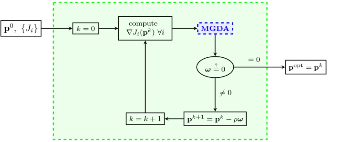
In this section we will focus on how to compute the research direction ω. That given, the
optimization algorithm will be the one illustrated in Figure 3.
p0, {J i} k= 0 ∇computeJi(pk)∀i MGDA ω= 0? pk+1=pk−ρω k=k+ 1 popt=pk 6 = 0 = 0
Figure 3: Flow chart of the optimization algorithm. The optimization loop is highlighted in green.
2.1
MGDA I and II: original method and first improvements
The original version of MGDA definesωas the minimum-norm element in the setU of the linear
convex combinations of the gradients:
U ={u∈RN :u= n X i=1 αi∇Ji(p), withαi≥0∀i, n X i=1 αi= 1}. (10)
In order to understand intuitively the idea behind this choice, let us analyse some two and three dimensional examples, shown in Figure 4 and Figure 5. The gradients can be seen as vectors of
RN all applied in the origin. Each vector identifies a pointxi∈RN, anddis the point identified
byω. In this framework,U is the convex hull of the pointsxi, highlighted in green in the Figures.
The convex hull lies in an affine subspace of dimension at mostn−1, denoted withAn−1 and
drawn in red. Note that ifn > N,An−1≡RN. We briefly recall the definition of projection on
O x1 x2 O⊥ ≡d ∇J2 ∇J1 ω U A1 O x1 x2≡d O⊥ ∇J2≡ω ∇J1 U A1 Figure 4: 2D examples. O x1 ∇J1 x2 ∇J2 x3 ∇J3 d≡O⊥ ω U O x1 ∇J1 x2 ∇J2 x3 ∇J3 O⊥ d ω U A2 Figure 5: 3D examples.
Definition 7. Let x be a point in a vector spaceV and letC ⊂V be a convex closed set. The
projectionof xonC is the pointz∈C such as:
z= argmin
y∈C
kx−ykV.
Given this definition, it is clear that finding the minimum-norm element in a set is equivalent
to finding the projection of the origin on this set. In the trivial caseO∈U (condition equivalent
to the Pareto stationarity), the algorithm givesω=0.
Otherwise, if O /∈ U, we split the projection procedure in two steps: first we project the
originOon the affine subspaceAn−1, obtainingO⊥; then, two scenarios are possible: ifO⊥∈U
thend≡O⊥ (as in the left subfigures) and we haveω, otherwise it is necessary to projectO⊥
onU findingdand, consequently,ω(as shown in the right subfigures).
Let us observe that in the special case in whichO⊥∈U, we are not “favouring” any gradients,
fact explained more rigorously in the following Proposition.
Proposition 4. If O⊥∈U, all the directional derivatives are equal along ω:
(ω,∇Ji(p)) =kωk2 ∀i= 1, . . . , n.
Proof. It is possible to write every gradient as the sum of two orthogonal vectors: ∇Ji(p) =
ω+vi, where vi is the vector connectingO⊥ andxi.
(ω,∇Ji(p)) = (ω,ω+vi) =
= (ω,ω) + (ω,vi) = (ω,ω) =kωk2.
The main limitation of this first version of the algorithm is the practical determination ofω
whenn >2. For more details on MGDA I, see [3].
In the second version of MGDA,ωis computed with a direct procedure, based on the
Gram-Schmidt orthogonalization process (see [19]), applied to rescaled gradients:
Ji0=
∇Ji(p) Si
.
However, this version has two main problems: the choice of the scaling factorsSiis very important
but arbitrary, and the gradients must be linearly independent to apply Gram-Schmidt, that is impossible, for instance, in a situation in which the number of gradients is greater than the
dimension of the space, i.e. n > N. Moreover, let us observe that in general the new ω
is different from the one computed with the first version of MGDA. For more details on this version of MGDA, see [4]. For these reasons, a third version has been introduced in [5].
2.2
MGDA III: algorithm for large number of criteria
2.2.1 Description
The main idea of this version of MGDA is that in the cases in which there are many gradients,
a common descent directionωcould be based on only a subset of gradients. Therefore, one can
consider only themost significant gradients, and perform an incomplete Gram-Schmidt process
on them. For instance, in Figure 6 there are seven different gradients, but two would be enough to compute a descent direction for all of them. In this contest, the ordering of the gradients is
0 g1 g2 g3 g4 g5 g6 g7 0 g1 g2 g3 g4 g5 g6 g7
Figure 6: 2D example of trends among the gradients. Two good vectors to compute a common descent direction could be the ones in red.
it will be mn. Let us observe that if the gradients live in a space of dimensionN, it will be,
for sure,m≤N. Moreover, this eliminates the problem of linear dependency of the gradients.
In this subsection we will indicate with{gi}ni=1the set of gradients evaluated at the current design
point p, corresponding respectively to the criteria {Ji}ni=1, and with {g(i)}n(i)=1 the reordered
gradients, evaluated atp, too. The ordering criterion proposed in [5] selects the first vector as
follows: g(1)=gk where k= argmax i=1,...,n min j=1,...,n (gi,gj) (gi,gi) , (11)
while the criterion for the following vectors will be shown afterwards. The meaning of this choice will be one of the subject of the next subsection.
Being the ordering criterion given, the algorithm briefly consists in: building the orthogonal
set of vectors{ui}mi=1by adding oneui at a time and using the Gram-Schmidt process; deciding
whether or not to add another vectorui+1 (i.e. stopping criterion); and, finally, computingωas
the minimum-norm element in the convex hull of {u1,u2, . . . ,um}:
ω= m X k=1 αkuk, whereαk = 1 1 + m X j=1 j6=k kukk2 kujk2 . (12)
The choice of the coefficientsαk will be justified afterwards.
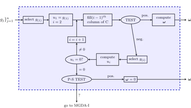
Now we analyse in detail some of the crucial part of the algorithm, with the support of the
flow chart in Figure 7. The algorithm is initialized as follows: first g(1) is selected (according
to (11)), then one impose u1 = g(1) and the loop starts with i = 2. In order to define the
stopping criterion of this loop (TEST in Figure 7), we introduce an auxiliary structure: the
lower-triangular matrix C. Letck,` be the element of the matrix C in thekth row,`thcolumn.
ck,` = (g(k),u`) (u`,u`) ` < k k−1 X `=1 ck,` `=k (13)
This matrix is set to0at the beginning of the algorithm, then is filled one column at a time (see
Figure 7). The main diagonal of the matrix C contains the sum of the elements in that row and
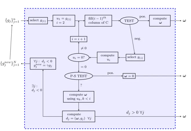
{gj}nj=1 selectg(1) u1=g(1) i= 2 fill(i−1)th column of C TEST pos. neg. compute ω ω i=i+ 1 ui= 0? 6 = 0 = 0 compute ui selectg(i) P-S TEST pos. ? ω= 0 ω go to MGDA-I
Figure 7: Flow chart of third version of MGDA
by the user and whose role will be studied in subsection 2.3.1, the test consists in checking if
c`,`≥a∀` > i: if it is true for all the coefficient the test is positive, the main loop is interrupted
and ω is computed as in (12) withm being the index of the current iteration, otherwise one
continues adding a newui computed as follows: first there is the identification of the index `
such as:
`= argmin
j=i,...,n
cj,j, (14)
then it is setg(i) =g` (these two steps correspond to “select g(i)” in Figure 7), and finally the
Gram-Schmidt process is applied:
ui = 1 Ai g(i)− X k<i ci,kuk ! , (15) whereAi:= 1− X k<i ci,k = 1−ci,i.
The meaning of the stop criterion is the following:
c`,`≥a >0 ⇒ ∃i: c`,i>0 ⇒ g\(`)ui∈ −π 2, π 2
This means that a descent direction forJ(`)can be defined from the{ui}already computed, and
adding a newucomputed on the base ofg(`) would not add much information.
Once computed a new ui, before adding it to the set, we should check if it is nonzero, as it is
shown in the flow chart. If it is zero, we know from the (15) that is:
g(i)= X
k<i
It is possible to substitute in cascade (15) in (16), obtaining: g(i)= X k<i ci,k " 1 Ak g(k)− X `<k ck,`u` !# = =X k<i ci,k 1 Ak g(k)− X `<k ck,` 1 A` g(`)− X j<` c`,juj = =. . . (17)
Therefore, since u1=g(1), one can write:
g(i)= X
k<i
c0i,kg(k) (18)
Computing thec0i,k is equivalent to solving the following linear system:
g(1) g(2) · · · g(i−1) | {z } =A c0 1,i c02,i ... ... c0i−1,i | {z } =x = g(i) | {z } =b
Since N is the dimension of the space in which the gradients live, i.e. gi ∈RN ∀i = 1, . . . , n,
the matrixAis[N×(i−1)], and for sure isi−1≤N, becausei−1is the number of linearly
independent gradients we already found. This means that the system is overdetermined, but we
know from (17)-(18) that the solution exists. In conclusion, to find the c0
i,k we can solve the
following system:
ATAx=ATb (19)
where ATA is a square matrix, and it is invertible because the columns of Aare linearly
inde-pendent (for further details on linear systems, see [19]). Once found the c0i,k, it is possible to
apply the Pareto-stationarity test (P-S TEST in Figure 7), based on the following Proposition. Proposition 5. c0i,k ≤0 ∀k= 1, . . . , i−1 ⇒Pareto-stationarity.
Proof. Starting from the (18), we can write:
g(i)− X k<i c0i,kg(k)= 0 ⇒ n X k=1 γkg(k)= 0 where: γk= −c0i,k k < i 1 k=i 0 k > i γk≥0 ∀k. If we defineΓ = n X k=1
γk, then the coefficients{γΓk}nk=1 satisfy the Definition 2.
Note that the condition given in Proposition 5 is sufficient, but not necessary. Therefore, if it is not satisfied we fall in an ambiguous case: the solution suggested in [5] is, in this case, to
2.2.2 Properties
We now present and prove some properties of MGDA III. Note that these properties are not valid if we fall in the ambiguous case.
Proposition 6. αi, i= 1, . . . , ndefined as in (12) are such that: m
X
k=1
αk = 1 and (ω,uk) =kωk2 ∀k= 1, . . . , m.
Proof. First, let us observe that:
1 αk = 1 + m X j=1 j6=k kukk2 kujk2 = kukk 2 kukk2 + m X j=1 j6=k kukk2 kujk2 = m X j=1 kukk2 kujk2 =kukk2 m X j=1 1 kujk2
Therefore, it follows that:
m X k=1 αk= m X k=1 1 kukk2 m X j=1 1 kujk2 = m X k=1 1/kukk2 m X j=1 1 kujk2 = m 1 X j=1 1 kujk2 m X k=1 1 kukk2 = 1.
Let us now prove the second part: (ω,ui) = m X k=1 αkuk,ui ! =αi(ui,ui) =αikuik2= 1 m X k=1 1 kukk2 =:D
where we used the definition ofω, the linearity of the scalar product, the orthogonality of the
ui and, finally, the definition ofαi. Let us observe that Ddoes not depend oni. Moreover,
kωk2= (ω,ω) = m X k=1 αkuk, m X `=1 α`u` ! = m X j=1 α2j(uj,uj) = = m X j=1 αjD=D m X j=1 αj =D= (ω,ui) ∀i= 1, . . . , m. Proposition 7. ∀i= 1, . . . , m (ω,g(i)) = (ω,ui).
Proof. From the definition ofui in (15), it is possible to writeg(i)in the following way:
g(i)=Aiui+ X k<i ci,kuk= 1− X k<i ci,k ! ui+ X k<i ci,kuk= =u − Xc ! u +Xc u
and doing the scalar product withωone obtains: (g(i),ω) = (ui,ω)− X k<i ci,k ! (ui,ω) + X k<i ci,kuk,ω ! | {z } =(?)
We want to prove that(?) = 0. As we have shown in the proof of Proposition 6:
αk= 1 kukk2 m X j=1 1 kujk2 ⇒ αikuik2= 1 m X j=1 1 kujk2
Using the definition ofω, the linearity of the scalar product and the orthogonality of theui one
obtains: (?) =− X k<i ci,k ! αikuik2+ X k<i ci,kαkkukk2= =− X k<i ci,k ! 1 Pm j=1 1 kujk2 + X k<i ci,k ! 1 Pm j=1 1 kujk2 = 0. Proposition 8. ∀i=m+ 1, . . . , n (g(i),ω)≥akωk2. Proof. It is possible to writeg(i) as follows:
m X
k=1
ci,kuk+vi
where vi⊥ {u1, . . . ,um}. Sincei > m, we are in the case in which the testci,i≥ais positive.
Consequently: (g(i),ω) = m X k=1 ci,k(uk,ω) = m X k=1 ci,kkωk2=ci,ikωk2≥akωk2.
In conclusion, as a straightforward consequence of the Propositions above, we have: (g(i),ω) =kωk2 ∀i= 1, . . . , m (g(i),ω)≥akωk2 ∀i=m+ 1, . . . , n,
which confirms that the method provides a direction that is a descent one even for the gradients not used in the construction of the Gram-Schmidt basis and, consequently, not directly used in
the computation ofω.
2.3
MGDA III b: Improvements related to the ambiguous case
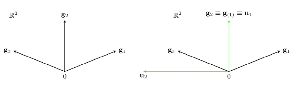
In this work we propose some strategies to avoid going back to MGDA-version I, when we fall in the ambiguous case, since it is very unefficient when a large number of objective functional are considered. In order to do this, we should investigate which are the reasons that lead to the ambiguous case. Let us observe that in the algorithm there are two arbitrary choices: the value
0 g1 g2 g3 R2 0 g1 g2≡g(1)≡u1 g3 u2 R2
Figure 8: Example to illustrate a wrong choice fora.
2.3.1 Choice of the threshold
Let us start with analysing how a too demanding choice of a (i.e. of a too large value) can
affect the algorithm. We will do this with the support of the example in Figure 8, following the algorithm as illustrated in the precedent subsection. For example, assume that the gradients are the following: g1= 5 2 g2= 0 5 g3= −5 2 . (20)
Using the criterion (11) the gradient selected as first isg2. At the first iteration of the loop the
first column of the matrixC is filled in as in (13), with the following result:
C= 1 0.4 0.4 0.4 0 0.4
If a is set, for instance, at 0.5 (or any value greater than 0.4) the stop test fails. However,
looking at the picture, it is intuitively clear thatω =u1 is the best descent direction one can
get (to be more rigorous, it is the descent direction that gives the largest estimate possible from
Proposition 8). If the test fails, the algorithm continues and another vectoruiis computed. This
particular case is symmetric, therefore the choice ofg(2) is not very interesting. Let us say that
g(2) =g3, than u2 is the one shown in the right side of Figure 20 and, since it is nonzero, the
algorithm continues filling another column ofC:
C= 1 0.4 0.4 0.4 −0.6 −0.2
Even in this case the stopping test fails (it would fail with any value ofa due to the negative
term in position (3,3)). Since we reached the dimension of the space, the nextui computed is
zero: this leads to the Pareto-stationarity test, that cannot give a positive answer, because we are not at a Pareto-stationary point. Therefore, we fall in the ambiguous case.
To understand why this happens, let us consider the relation between a and ω, given by
Proposition 8 that we briefly recall:
∀i=m+ 1, . . . , n (g(i),ω)≥akωk2.
This means that, for the gradients that haven’t been used to computeω, we have a lower bound
that it is impossible to know a priori how biga can be. For this reason, the parameter a has
been removed. The stopping test remains the same as before, with only one difference: instead
of checkingc`,`≥aone checks ifc`,`>0.
However, removingais not sufficient to remove completely the ambiguous case, as it is shown
in the next subsubsection.
2.3.2 Ordering criteria
In this subsection we will analyse the meaning of the ordering criterion used in MGDA III and we will present another one, providing some two-dimensional examples in order to have a concrete idea of different situations.
The ordering problem can be divided in two steps:
(i) choice ofg(1)
(ii) choice ofg(i), giveng(k) ∀k= 1, . . . i−1
The naïve idea is to order the gradients in the way that makes the MGDA stop as soon as possible. Moreover, we would like to find an ordering criterion that minimizes the times in which
we fall in the ambiguous case (i.e. when we find aui= 0and the P-S test is not satisfied).
Definition 8. Let us say that an ordering is acceptable if it does not lead to the ambiguous case, otherwise we say that the ordering is not acceptable.
First, we discuss point (ii), since it is simpler. If we are in the case in which we have to add another vector, it is because the stopping test gave a negative result, therefore:
∃`, i≤`≤n: c`,`<0.
We chose asg(i) the one that violates the stopping test the most. This explains the (14), that
we recall here:
g(i)=gk : k= argmin
`
c`,` i≤`≤n.
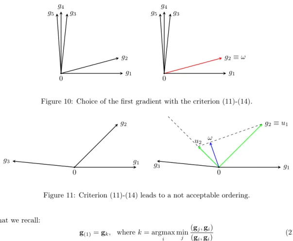
The point (i) is more delicate, since the choice of the first vector influences strongly all the following choices. Intuitively, in a situation like the one shown in Figure 9, we would pick as first
vectorg5 and we would have the stopping test satisfied at the first iteration, in fact ω=g5 is
a descent direction for all the gradients. Formally, this could be achieved using the criterion 11,
0 g1 g2 g3 g4 g5 g6 g7 g8 g9 0 g1 g2 g3 g4 g5 g6 g7 g8 g9 Figure 9: Example 1.
0 g1 g2 g3 g4 g5 0 g1 g2≡ω g3 g4 g5
Figure 10: Choice of the first gradient with the criterion (11)-(14).
0 g1 g2 g3 0 g1 g2≡u1 g3 u2 ω
Figure 11: Criterion (11)-(14) leads to a not acceptable ordering. that we recall: g(1)=gk, wherek= argmax i min j (gj,gi) (gi,gi) (21)
However, it is clear that this is not the best choice possible in cases like the one shown in Figure 10, in which none of the gradients is close to the bisecting line (or, in three dimensions, to the axis of the cone generated by the vectors). In this particular case, it would be better to
pick two external vectors (g1 and g5) to compute ω. Anyway, with the criterion (11)-(14) we
still obtain anacceptableordering, and the descent direction is computed with just one iteration.
However, there are cases in which the criterion (11)-(14) leads to anot acceptable ordering. Let
us consider, for example, a simple situation like the one in Figure 11, with just three vectors, and let us follow the algorithm step by step.
Let the gradients be the following:
g1= 1 0 g2= 0.7 0.7 g3= −1 0.1 (22)
Given the vectors (22), we can build a matrixT such as:
[T]i,j= (gj,gi) (gi,gi) (23) obtaining: T = 1 0.7 −1 0.714 1 −0.643 −0.99 −0.624 1 min=−1 min=−0.643 min=−0.99
{gj}nj=1 selectg(1) u1=g(1) i= 2 fill(i−1)th column of C TEST pos. neg. compute ω ω i=i+ 1 ui= 0? 6 = 0 = 0 compute ui selectg(i) P-S TEST pos. ? ω= 0 ω computeω usinguk, k < i compute dj= (ω, gj) ∀j ω dj >0 ∀j ∀j: dj<0 gnew j =γgj ∃j: dj<0 {gnew j }Nj=1
Figure 12: Flow chart of MGDA-III b
The internal minimum of (11) is the minimum of each row. Among this, we should select the
maximum: the index of this identifies the indexksuch asg(1)=gk. In this case,k= 2. We can
now fill in the first column of the triangular matrixC introduced in (13), obtaining:
C= 1 0.714 0.714 −0.642 0 −0.642
Since the diagonal terms are not all positive, we continue adding g(2) =g3, according to (14).
Note that, due to this choice, the second line of the matrix C has to be switched with the
third. The next vector of the orthogonal baseu2 is computed as in (15), and in Figure 11, right
subfigure, it is shown the result. Having a newu26=0, we can now fill the second column ofC
as follows: C= 1 −0.642 −0.642 0.714 −1.4935 −0.77922
This is a situation analogue to the one examinated in the example of subsection 2.3.1, therefore we fall in the ambiguous case.
A possible solution to this problem is the one proposed in the flow chart in Figure 12: compute
ωwith the{ui}that we already have and check for which gradients it is not a descent direction
(in this case forg1, as shown in the right side of Figure 11). We want this gradient to be “more
0 g1≡u1
g2
g3 u
2ω
Figure 13: Criterion (11)-(14) after doubling.
beginning. This leads to a different matrixT:
T = 1 0.35 −0.5 1.428 1 −0.643 −1.98 −0.624 1 min=−0.5 min=−0.643 min=−1.98
With the same process described above, one obtainsg(1)=u1=g1. The final output of MGDA
is shown in Figure 13, withω= [0.00222,0.0666]T.
However, rerunning MGDA from the beginning is not an efficient solution, in particular in the cases in which we have to do it many times before reaching a good ordering of the gradients. For this reason, a different ordering criterion is proposed: we chose as a first vector the “most external”, or the “most isolated” one. Formally, this means:
g(1)=gk, wherek= argmin i min j (gj,gi) (gi,gi) (24)
On one hand with this criterion it is very unlikely to stop at the first iteration, but on the other hand the number of situations in which is necessary to rerun the whole algorithm is reduced. Note that, in this case, instead of doubling the length of the non-considered gradients, we must make the new gradients smaller.
These solutions are not the only ones possible, moreover there is no proof that the ambiguous case is completely avoided. For instance, another idea could be the following: keeping the
threshold parameterafor the stopping test and, every time the ambiguous case occurs, rerunning
3
Numerical methods for state and sensitivity analyses
In this section, first we will illustrate the general solving procedure that has been applied to solve multi-objective optimization problems with PDE constraints, then we will introduce the specific PDEs used as test cases in this work and finally we will present the first numerical results, related to the convergence of the schemes and the validation of the methods used.
3.1
Solving method
In this subsection we want to explain the method used in this work to solve problem of the kind (6). First, let us recall all the ingredients of the problem:
· state equation: ∂u ∂t +L(u) =s(x, t;p) x∈Ω, 0< t≤T ∇u·n= 0 ΓN ⊆∂Ω, 0< t≤T u=f(t) ΓD⊆∂Ω, 0< t≤T u=g(x) x∈Ω, t= 0
· cost functionalJ that we assume quadratic inu:
J(u(p)) = 1
2q(u, u), (25)
where q(·,·)is a bilinear, symmetric and continuous form. For instance, a very common
choice forJ in problems of fluid dynamics isJ = 12k∇uk2
L2(Ω).
Let us observe that every classical optimization method requires the computation of the gradient
of the cost functional with respect to the parametersp, that we will indicate with ∇J. In order
to compute it, we can apply the chain rule, obtaining:
∇J(p0) =d(J◦u)(p0) =dJ(u0)◦du(p0),
beingu0=u(p0). Therefore,∇J is composed by two pieces. Let us start analysing the first one.
Proposition 9. If J is like in (25), than its Fréchet differential computed inu0 and applied to the generic incrementhis:
dJ(u0)h=q(u0, h)
Proof. Using the definition of Fréchet derivative one obtains: J(u0+h)−J(u0) = 1 2q(u0+h, u0+h)− 1 2q(u0, u0) = =q(u0, h) + 1 2q(h, h) =q(u0, h) +O(khk 2),
where the last passage is justified by the continuity of q(·,·).
The second piece, i.e. du(p0), is just the derivative ofuwith respect to the parameters. This
means that thei−thcomponent of the gradient ofJ is the following:
[∇J(p0)]i=q u0, upi(p
0)
where
upi(p
0) = ∂u ∂pi
(p0),
and it is calledsensitivity (with respect to the parameterpi). We now apply this procedure to
the example introduced above,J = 1
2k∇uk 2
L2(Ω). We observe that the formqis:
q(u, v) = (∇u,∇v)L2(Ω),
that is bilinear, symmetric and continuous. Therefore we can apply the result of Proposition 9, obtaining:
[∇J(p0)]i= ∇u0,∇upi(p
0) L2(Ω).
Summing up: in order to solve a minimization problem like (6), we need to compute the
gradient ofJ with respect to the parameters. To do that, we see from (26) that it is necessary to
knowu0=u(p0)(therefore to solve the state equation withp=p0) and to know upi. The last
step we have to do is finding the equations governing the behaviour of the sensitivitiesupi. To do
that, we apply theContinuous Sensitivity Equation method, shorten in CSE method from now
on. See [9]. It consists in formally differentiating the state equation, the boundary and initial
condition, with respect topi:
∂ ∂pi ∂u ∂t +L(u) = ∂p∂ is(x, t;p) x∈Ω, 0< t≤T ∂ ∂pi(∇u·n) = 0 ΓN ⊆∂Ω, 0< t≤T ∂ ∂piu= 0 ΓD⊆∂Ω, 0< t≤T ∂ ∂piu= 0 x∈Ω, t= 0.
After a permutation of the derivatives, if Lis linear and Ωdoes not depend onp, one obtains
thesensitivities equations: ∂upi ∂t +L(upi) =spi(x, t;p) x∈Ω, 0< t≤T ∇upi·n= 0 ΓN ⊆∂Ω, 0< t≤T upi = 0 ΓD⊆∂Ω, 0< t≤T upi = 0 x∈Ω, t= 0. (27)
For everyi= 1, . . . , N, this is a problem of the same kind of the state equation and independent
from it, therefore from a computational point of view it is possible to use the same solver and
to solve theN+ 1problems in parallel (N sensitivity problems plus the state). However, ifLis
nonlinear,
L(upi)6=
∂ ∂pi
L(u),
and we need to introduce a new operatorLe=L(e u, upi) =
∂
∂piL(u). Therefore, the sensitivities
equations in this case will be:
∂upi ∂t +L(eu, upi) =spi(x, t;p) x∈Ω, 0< t≤T ∇upi·n= 0 ΓN ⊆∂Ω, 0< t≤T upi= 0 ΓD⊆∂Ω, 0< t≤T upi= 0 x∈Ω, t= 0. (28) They are no more independent from the state equation, but they remain independent ones from the others. Let us observe that in this case it is necessary to implement a different (but similar) solver than the one used for the state.
3.2
Test cases
In this work we will consider only unsteady one-dimensional scalar advection-diffusion PDEs,
both linear and nonlinear. Let Ω = (xa, xb) be the domain. The linear equation will be the
following: ∂tu−b∂x2u+c∂xu=s(x, t;p) in(xa, xb), 0< t≤T u(xa, t) =fD(t) 0< t≤T ∂xu(xb, t) =fN(t) 0< t≤T u(x,0) =g(x) in(xa, xb) (29)
where b andc are constant coefficients b, c >0, cb (i.e. dominant advection), s(x, t), fD(t),
fN(t) and g(x) are given functions and pis the vector of control parameters. Being c > 0 it
makes sense to impose Dirichlet boundary condition in xa, since it is the inlet, and Neumann
boundary condition inxb, since it is the outlet. We observe that the problem (29) is well posed,
i.e. the solution exists and is unique. For more details on the well posedness of this kind of problems see [18], [14].
Applying the CSE method, introduced in subsection 3.1, one obtains the following sensitivity
equations, for every i= 1, . . . , N:
∂tupi−b∂ 2 xupi+c∂xupi =spi(x, t;p) in(xa, xb), 0< t≤T upi(xa, t) = 0 0< t≤T ∂xupi(xb, t) = 0 0< t≤T upi(x,0) = 0 in(xa, xb) (30)
Let us observe that the sensitivity equations (30) are independent one from the other and all from the state. Moreover, the same solver can be used for all of them.
On the other hand, for the nonlinear case we consider the following equation:
∂tu−b∂x2u+cu∂xu=s(x, t;p) in(xa, xb), 0< t≤T u(xa, t) =fD(t) 0< t≤T ∂xu(xb, t) =fN(t) 0< t≤T u(x,0) =g(x) in(xa, xb). (31)
We will impose source term, initial and boundary condition such asu(x, t)>0∀x∈(xa, xb), ∀t∈
(0, T). In this way the advection fieldcuis such thatxais always the inlet andxb the outlet, and
we can keep the same boundary condition and, most important thing, the same upwind scheme for the convective term, introduced in the next subsection. However, in this case the sensitivity equations are: ∂tupi−b∂ 2 xupi+cu∂xupi+cupi∂xu=spi(x, t;p) in(xa, xb), 0< t≤T upi(xa, t) = 0 0< t≤T ∂xupi(xb, t) = 0 0< t≤T upi(x,0) = 0 in(xa, xb). (32)
These are linear PDEs of reaction-advection-diffusion with the advection coefficientcu(x, t)and
the reaction coefficientc∂xu(x, t)depending on space and time. In this case it is not possible to
use the same solver for state and sensitivity, moreover the sensitivity equations depend on the solution of the state.
3.3
Numerical schemes
We now introduce the numerical schemes used to solve the problems (29)-(30)-(31)-(32). In every
case, the space has been discretized with a uniform grid{xi}Ni=0 wherexi=xa+i∆xand∆xis
the spatial step, that can be chosen by the user.
x0 x1 x2 x3 . . . xN−1 xN
∆x
Also in time, we considered a uniform discretization: {tn}K
n=0 wheretn =n∆tand∆tis chosen
such as two stability conditions are satisfied: ∆t < 1 2 ∆x2 b ∧ ∆t < ∆x c . (33)
These conditions (33) are necessary, since we use explicit methods in time, as shown in the next subsubsections.
A first order and a second order scheme have been implemented, by using finite differences in space for both orders, while in time explicit Euler for first order, and a Runge-Kutta scheme for second order. See [14] and [10] for more details on these schemes. The resulting schemes are the following:
all of them are initialized using the initial condition and the Dirichlet boundary condition:
u0i =g(xi) ∀i= 0, . . . , N un0 =fD(tn) ∀n= 0, . . . , K.
• First order scheme for the linear case∀ n= 1, . . . , K, ∀i= 1, . . . , N −1:
uni+1=uni −∆t c u n i −uni−1 ∆x + ∆t b un i+1−2uni +uni−1 ∆x2 + ∆t s(xi, t n) (34)
Neumann boundary conditioni=N:
unN+1=unN+1−1+ ∆xfN(tn+1)
• Second order scheme for the linear case∀n= 1, . . . , K, ∀i= 2, . . . , N−1:
un+ 1 2 i =uni − ∆t 2 c 3un i−4uni−1+uni−2 2∆x + ∆t 2 b un i+1−2uni+uni−1 ∆x2 + ∆t 2 s(xi, t n) uni+1=un i −∆t c 3un+ 12 i −4u n+ 12 i−1 +u n+ 12 i−2 2∆x + +∆t b u n+ 12 i+1 −2u n+ 12 i +u n+ 12 i−1 ∆x2 + ∆t s(xi, tn+ 1 2) (35)
Neumann boundary conditioni=N:
unN+1= 1 3(4u n+1 N−1−u n+1 N−2+ 2∆x fN(tn+1))
Since the numerical dependency stencil for the internal nodes (∀i= 1, . . . , N−1) is the
un+12 i−2 u n+1 2 i−1 u n+1 2 i u n+1 2 i+1 uni+1 ∆t 2 ∆x
for the computation ofun1+1 it is necessary to know the value of the solution in a point
outside the domain. Different choices for this node lead to different schemes. Unless
otherwise indicated, in this work we decided to imposeun
−1=un0.
With these two schemes (34)-(35) it is possible to solve the linear state equation (29) and the linear sensitivity equations (30).
For the nonlinear state equation (31) the scheme is very similar to the one shown above, the only difference is in the advection term.
• First order scheme for the nonlinear case∀ n= 1, . . . , K, ∀i= 1, . . . , N −1:
uni+1=uni −∆t cuni u n i −uni−1 ∆x + ∆t b un i+1−2uni +uni−1 ∆x2 + ∆t s(xi, t n) (36)
• Second order scheme for the nonlinear case∀n= 1, . . . , K, ∀ i= 2, . . . , N−1:
un+ 1 2 i =uni − ∆t 2 cu n i 3un i−4uni−1+uni−2 2∆x + ∆t 2 b un i+1−2uni+uni−1 ∆x2 + ∆t 2 s(xi, t n) uni+1=un i −∆t cu n+1 2 i 3un+ 12 i −4u n+ 12 i−1 +u n+ 12 i−2 2∆x + +∆t b u n+ 12 i+1 −2u n+ 12 i +u n+ 12 i−1 ∆x2 + ∆t s(xi, tn+ 1 2) (37)
Note that, since the numerical dependency stencil is the same as in the linear case, we have
the same problem for computation of the solution in the first nodex1.
Finally, to solve the equation (32), the linear schemes can be used, with two simple
modifi-cation. The first one is that the coefficient c, constant in (34)-(35), has to be substituted with
cn
i in (34) and in the first equation of (35), and withc
n+1 2
i in the second equation of (37), being
cn
i 'cu(xi, tn). Note that the equation is linear since we are solving the sensitivity equations in
upk andu(x, t)is given. The second one is that the reaction termc(∂xu)
n i(upk)
n
i must be added.
Let us observe that in this case, for the second order scheme, it is necessary to know the stateu
on a temporal grid twice as fine as the one used for the sensitivity equations.
3.4
Verification of the state analysis
In this subsection we will present some numerical convergence results in order to verify the actual order of the finite differences schemes in some simple cases. This subsection is not meant to be exhaustive on the convergence topic, but only a brief check in some simple cases in which it is easy to compute the analytical solution. First let us observe that the discretization of the diffusion term does not change from the first to the second order scheme, therefore we focused on only advection problems.
3.4.1 Advection problem with a steady solution The first simple case is the following:
∂tu+c ∂xu=x in(0,1), 0< t≤T u(0, t) = 0 0< t≤T u(x,0) = 0 in(0,1). (38) Since both the source term and the Dirichlet boundary condition do not depend on time, there
will be a steady solution, that isuex= x
2
2c. If the final time T is big enough, also the numerical
solution will be steady. The error is computed as follows:
e(T) =kuex(x, T)−uh(x, T)kL2(0,1),
whereuex is the exact solution anduh the numerical solution. In Figure 14 is shown the error
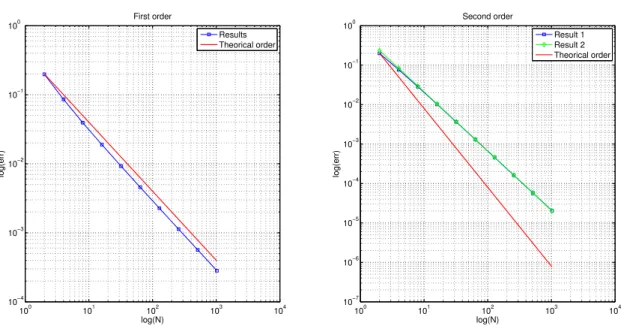
✶ ✵ ✶ ✁ ✶ ✷ ✶ ✸ ✶ ✹ ✶ ✲✹ ✶ ✲✸ ✶ ✲✷ ✶ ✲✁ ✶ ✵ ❧✂✄ ☎✆✝ ✞ ✟ ✠ ✡ ☛ ☞ ☞ ✌ ❋ ✍✎✏✑✂✎✒✓ ✎ ❘✓ ✏✔❧✑✏ ❚✕✓✂✎✍✖✗ ❧✂✎✒✓ ✎ ✶ ✵ ✶ ✁ ✶ ✷ ✶ ✸ ✶ ✹ ✶ ✲✘ ✶ ✲✙ ✶ ✲✚ ✶ ✲✹ ✶ ✲✸ ✶ ✲✷ ✶ ✲✁ ✶ ✵ ❙✓✖✂✛ ✒✂✎✒✓ ✎ ❧✂✄ ☎✆✝ ✞ ✟ ✠ ✡ ☛ ☞ ☞ ✌ ❘✓✏✔❧✑✶ ❘✓✏✔❧✑✜ ❚✕✓✂✎✍✖✗❧✂✎✒✓✎
Figure 14: Convergence advection steady problem
with respect to the grid: the theoretical slope is in red. The first order scheme has the expected convergence. For the second order, two different results are plotted: the green one correspond
to the choice of un
−1=uex(−∆x, tn), the blue one to un−1=fD(tn). As one can notice, the
difference is not significant. However, in both cases the order is not the one expected. This can be explained by the fact that numerically we are imposing two boundary condition to a problem that requires only one. The results obtained removing the Neumann boundary condition and imposing in the last node the same scheme of the internal nodes are shown in Figure 15. These
results show that the order is the one expected if we useun−1=fD(tn), otherwise, using the exact
solution for the external node leads to a problem that is too simple: the error is comparable to
the machine error for all the grids. In fact, we are imposing the exact solution in two nodes (x−1
and x0). Moreover, developing by hand the scheme for the computation of un1 and imposing
un i =u
n+1
i (because of the stationarity), one finds that the scheme yieldsu1=
∆x2
2c , that is the
exact solution in x1. Since uex is a parabola, two nodes inside the domain (plus the external
✶ ✵ ✶ ✁ ✶ ✷ ✶ ✸ ✶ ✹ ✶ ✲✁✂ ✶ ✲✁✄ ✶ ✲✁✹ ✶ ✲✁✷ ✶ ✲✁✵ ✶ ✲ ✂ ✶ ✲✄ ✶ ✲✹ ✶ ✲✷ ✶ ✵ ❧ ☎✆✝✞ ✟ ✠✡ ☛ ☞ ✌ ✍ ✍ ✎ ❘✏ ✑✒❧ ✓✶ ❘✏ ✑✒❧ ✓✔ ❚✕✏☎✖✗✘✙❧
Figure 15: Convergence advection steady problem, without Neumann boundary condition
3.4.2 Advection unsteady problem
The second simple case considered is the following:
∂tu+c ∂xu= 0 in(0,1), 0< t≤T u(0, t) = 1 +αsin(f t) 0< t≤T u(x,0) = 0 in(0,1). (39)
Let us observe that the function u(x, t) = 1 +αsin(f(ct−x)) satisfies the equation and the
boundary condition. Moreover, if the time t is big enough (let us say t > t), the influence of
the initial condition is negligible. The results shown in this subsection are obtained with c= 1,
f = 32π,t= 3 andT = 6. The error is computed as follows:
e(t) =kuex(x, t)−uh(x, t)kL2(0,1) err=ke(t)kL∞(t,T),
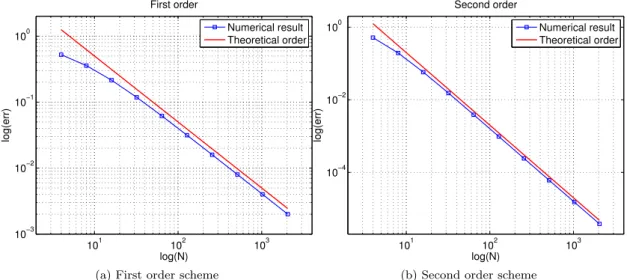
and it is shown in Figure 16 with respect to the grid. On the left there is the first order scheme, on the right the second order. The theoretical slope is in red: when the grid becomes fine enough, both schemes have the order expected, for every time considered.
101 102 103 10−3 10−2 10−1 100 log(N) log(err) First order Numerical result Theoretical order
(a) First order scheme
101 102 103 10−4 10−2 100 Second order log(N) log(err) Numerical result Theoretical order
(b) Second order scheme
Figure 16: Convergence advection unsteady problem.
3.5
Consistency of the sensitivity analysis
The purpose of this subsection is to validate the CSE method introduced in subsection 3.1. To do that, we will consider the problems (29) and (31) with specific boundary and initial conditions:
fD(t) =k+αsin(2πf t) fN(t)≡0 g(x)≡k (40)
whereαandf are given parameters,k is big enough to guaranteeu(x, t)≥0. We consider the
following source term:
s(x, t) = (√ Asin(2πf t+ϕ) sin2(x−xc L π− π 2), ifx∈(xc− L 2, xc+ L 2) 0, otherwise (41)
where L is the width of the spatial support, xc is the centre of the support and A and ϕ are
the design parameters, therefore we havep= (A, ϕ). The source term at some sample times is
shown below. xc 1 L x Source term t1 t2 t3 t4
These being the conditions of the state equation, we now introduce the source terms of the sensitivity equations (30) and (32):
sA(x, t) = ( 1 2√A sin(2πf t+ϕ) sin 2 (x−xc L π− π 2), ifx∈(xc− L 2, xc+ L 2) 0 otherwise (42) and sϕ(x, t) = (√ A cos(2πf t+ϕ) sin2(x−xc L π− π 2), ifx∈(xc− L 2, xc+ L 2) 0 otherwise. (43)
Note that one must solve each problem ((30) and (32)) twice: once with (42) as source term, and once with (43). To validate the method, we observe that a first order Taylor expansion of the solution with respect to the parameters gives:
u(A+dA, ϕ) =u(A, ϕ) +dA uA(A, ϕ) +O(dA2), (44a)
u(A, ϕ+dϕ) =u(A, ϕ) +dϕ uϕ(A, ϕ) +O(dϕ2). (44b)
We now defineuF D as the solution computed with the finite differences scheme, anduCSE as an
approximation of the solution obtained as follows:
uCSE(x, t;pi+dpi) =u(x, t;pi) +dpiupi(x, t;pi),
where pi can be either A orϕ, and u(x, t;pi)is called reference solution. We want to measure
the following quantity:
diff(T) :=kuF D(x, T)−uCSE(x, T)kL2(0,1),
and we expect, due to the Taylor expansion (44), that it will be diff(T)'O(dp2
i). To do that, we
varied the design parameters one at a time, following the procedure illustrated in Algorithm 1.
Figure 17 shows in a logarithmic scale diffA(on the left) and diffϕ(on the right), computed as in
Algorithm 1 Validation of the CSE method
1: A←Arefer,ϕ←ϕrefer
2: r←rstart . r=ratio= dA
A =
dϕ ϕ
3: solve state equation with(A, ϕ)−→store solution inurefer
4: solve sensitivity equations with(A, ϕ)−→store solutions inuA, uϕ
5: fork= 0. . . N do
6: dA←rA,dϕ←rϕ
7: solve state equation with(A+dA, ϕ)−→store solution inuA+dA
8: solve state equation with(A, ϕ+dϕ)−→store solution inuϕ+dϕ
9: diffA[k]← kuA+dA(x, T)−urefer(x, T)−dAuA(x, T)kL2(0,1)
10: diffϕ[k]← kuϕ+dϕ(x, T)−urefer(x, T)−dϕuϕ(x, T)kL2(0,1)
11: r∗= 2
12: end for
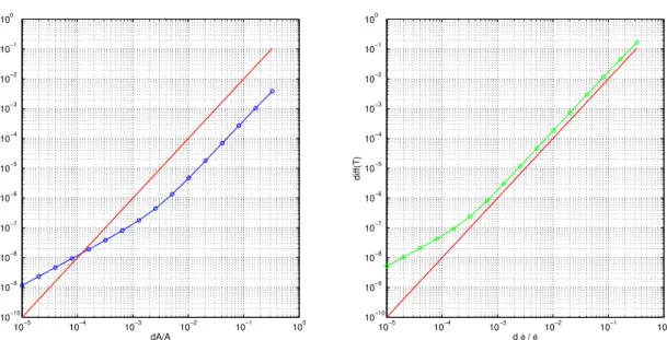
line 9-10, Algorithm 1, for the linear case. The red line is the theoretical slope. Figure 18 shows the same results for the nonlinear case. One can notice that, in the nonlinear case, the slope is the one expected only starting from a certain threshold. This is due to the approach chosen in this work, “differentiate, then discretize”, opposed to the other possible approach “discretize, then
✶ ✲✁ ✶ ✲✂ ✶ ✲✄ ✶ ✲☎ ✶ ✲✆ ✶ ✵ ✶ ✲✆ ☎ ✶ ✲✆ ✵ ✶ ✲✝ ✶ ✲✞ ✶ ✲✂ ✶ ✲ ☎ ✶ ✵ ❞ ✟✠ ✟ ✡ ☛ ☞ ☞ ✌ ✍ ✎ ❞ ✏ ✑ ✑ ❆ ❈❞✟ ✷ ✶ ✲✁ ✶ ✲✂ ✶ ✲✄ ✶ ✲ ☎ ✶ ✲✆ ✶ ✵ ✶ ✲✆ ✵ ✶ ✲✒ ✶ ✲✝ ✶ ✲✓ ✶ ✲✞ ✶ ✲✁ ✶ ✲✂ ✶ ✲ ✄ ✶ ✲ ☎ ✶ ✲✆ ✶ ✵ ❞❢✠❢ ✡ ☛ ☞ ☞ ✌ ✍ ✎ ❞✏✑✑ ✔ ❈❞❢ ✷
Figure 17: Validation of the CSE method, linear case. On the left diffA, on the right diffϕ. In
red the theoretical slope.
✶ ✲✁ ✶ ✲✂ ✶ ✲✄ ✶ ✲☎ ✶ ✲✆ ✶ ✵ ✶ ✲✆ ✵ ✶ ✲✝ ✶ ✲✞ ✶ ✲✟ ✶ ✲✠ ✶ ✲✁ ✶ ✲✂ ✶ ✲ ✄ ✶ ✲ ☎ ✶ ✲✆ ✶ ✵ ❞ ✡☛ ✡ ☞ ✌ ✍ ✍ ✎ ✏ ✑ ✶ ✲✁ ✶ ✲✂ ✶ ✲✄ ✶ ✲ ☎ ✶ ✲✆ ✶ ✵ ✶ ✲✆ ✵ ✶ ✲✝ ✶ ✲✞ ✶ ✲✟ ✶ ✲✠ ✶ ✲✁ ✶ ✲✂ ✶ ✲ ✄ ✶ ✲ ☎ ✶ ✲✆ ✶ ✵ ❞❢☛❢ ☞ ✌ ✍ ✍ ✎ ✏ ✑
Figure 18: Validation of the CSE method, nonlinear case. On the left diffA, on the right diffϕ.
differentiate”: in fact Taylor expansion (44) is carried out on the exact solution. By discretizing the equations, one adds discretization error, so:
diff(T) =O(dp2i) +O(hr),
whereris the order of the scheme used. The change of slope of the numerical results in Figure 18
corresponds to the point in whichO(hr)gets comparable withO(dp2
i). Note that in this case a
spatial step∆x= 0.05has been used.
On the contrary, in the “discretize, then differentiate” approach, the Taylor expansion is consistent with the numerical solution computed, whatever grid is used. In the linear case, one can notice that both approaches yield to the same solution, which explains the results.
4
Numerical results
In this section we present the numerical results obtained by applying MGDA III b, to problems governed by PDEs like (29) and (31), by following the procedure described in subsection 3.1.
First of all, we need to introduce the time dependent cost functionalJ. The sameJ has been
used in all the test cases, and it is the one introduced, as an example, in subsection 3.1, i.e.:
J(p) =1 2k∇u(p)k 2 L2(Ω)= 1 2(∇u(p),∇u(p))L2(Ω). (45)
We also recall that in this case the gradient ofJ with respect to the parameters is:
∇J(p) = (∇u(p),∇upi(p))L2(Ω), (46)
whose computation requires to solve the state and the sensitivity equations.
First we will present some results obtained with theinstantaneous approach, that means, we
define the set of objective functionals as:
Jk(p) =J(u(tk;p)) ∀k= 1, . . . , n,
later, we will present a result obtained with thewindows approach, where:
Jk(p) = Z tk+1
tk
J(u(t;p))dt ∀k= 1, . . . , n.
The solving procedure is schematically recalled in the Algorithm 2, in the case of instantaneous approach. Note that the algorithm is general, the only significant difference for the windows
approach is in the evaluation of the cost functionalsJk (line 8).
In subsection 3.5 we introduced some specific source terms, boundary and initial conditions: unless otherwise indicated, all the results of this subsection are obtained with the same data, with fixed values of the non-optimized parameters, reported in Table 1.
Table 1: Values of non-optimized parameters
Parameter Symbol Value
frequency f 4
source centre xc 0.2
source width L 0.2
b.c. average k 5
b.c amplitude α 1
These choices for the values of the parameters are related to the choice of the time and grid steps: in order to have a spatial grid fine enough to represent accurately the source term we chose
∆x= L
20,
that is, being L= 0.2, ∆x = 0.01. For the temporal step, we recall that it has to satisfy the
stability condition (33).
As we said in the first subsection, unless all the cost functionals have their minimum in the same point, there is not a unique optimal solution: this means that running the multi-objective