SFB 649 Discussion Paper 2010-055
S
FB
6
4
9
E
C
O
N
O
M
I
C
R
I
S
K
B
E
R
L
I
N
Capturing the Zero:
A New Class of
Zero-Augmented Distributions
and Multiplicative Error
Processes
Nikolaus Hautsch*
Peter Malec*
Melanie Schienle*
* Humboldt-Universität zu Berlin, Germany
This research was supported by the Deutsche
Forschungsgemeinschaft through the SFB 649 "Economic Risk". http://sfb649.wiwi.hu-berlin.de
ISSN 1860-5664
SFB 649, Humboldt-Universität zu Berlin Spandauer Straße 1, D-10178 Berlin
Capturing the Zero: A New Class of Zero-Augmented
Distributions and Multiplicative Error Processes
∗Nikolaus Hautsch† Peter Malec‡ Melanie Schienle§ November 2010
Abstract
We propose a novel approach to model serially dependent positive-valued vari-ables which realize a non-trivial proportion of zero outcomes. This is a typical phenomenon in financial time series observed on high frequencies, such as cumulated trading volumes or the time between potentially simultaneously occurring market events. We introduce a flexible point-mass mixture distribution and develop a semiparametric specification test explicitly tailored for such distributions. More-over, we propose a new type of multiplicative error model (MEM) based on a zero-augmented distribution, which incorporates an autoregressive binary choice component and thus captures the (potentially different) dynamics of both zero occurrences and of strictly positive realizations. Applying the proposed model to high-frequency cumulated trading volumes of liquid NYSE stocks, we show that the model captures both the dynamic and distribution properties of the data very
∗
For helpful comments and discussions we thank the participants of workshops at Humboldt-Universit¨at zu Berlin. This research is supported by the Deutsche Forschungsgemeinschaft (DFG) via the Collaborative Research Center 649 ”Economic Risk”.
†
Institute for Statistics and Econometrics and Center for Applied Statistics and Economics (CASE), Humboldt-Universit¨at zu Berlin as well as Quantitative Products Laboratory (QPL), Berlin, and Center for Financial Studies (CFS), Frankfurt. Email: [email protected]. Address: Spandauer Str. 1, D-10178 Berlin, Germany.
‡
Corresponding author. Institute for Statistics and Econometrics, Humboldt-Universit¨at zu Berlin. Email: [email protected]. Address: Spandauer Str. 1, D-10178 Berlin, Germany.
§
Institute for Statistics and Econometrics and Center for Applied Statistics and Economics (CASE), Humboldt-Universit¨at zu Berlin. Email: [email protected]. Address: Spandauer Str. 1, D-10178 Berlin, Germany.
well and is able to correctly predict future distributions.
Keywords: high-frequency data, point-mass mixture, multiplicative error model, excess zeros, semiparametric specification test, market microstructure
JEL classification: C22, C25, C14, C16, C51
1
Introduction
The availability and increasing importance of high-frequency data in empirical finance and financial practice has triggered the development of new types of econometric models capturing the specific properties of these observations. Typical features of financial data observed on high frequencies are strong serial dependencies, irregular spacing in time, price discreteness and the non-negativity of various (trading) variables. To account for these properties, models have been developed which contain features of both time series approaches and microeconometric specifications, see, e.g., Engle and Russell(1998), Russell and Engle (2005) or Rydberg and Shephard(2003), among others.
This paper proposes a novel type of model capturing a further important property of high-frequency data which is present in many situations but not taken into account in extant approaches: the occurrence of a non-trivial part of zeros in the data – henceforth referred to as ”excess zeros” – which is a typical phenomenon in both irregularly-spaced as well as aggregated (regularly spaced) financial time series on high frequencies. For instance, when modeling trade durations, many transaction data sets reveal a high proportion of simultaneous occurrences of trades (and thus zero durations). They are induced either by (large) trades which are simultaneously executed against several (small) orders, by imprecise recording which assigns identical time stamps to fast sequences of trades1 or by actual simultaneous occurrences of trading events. As it is mostly quite difficult or even impossible to exactly identify and to disentangle such effects, the often employed pragmatic solution of just aggregating all simultaneous events together – and thus ultimately discarding zero occurrences – is not appropriate. A further example, which serves as the major motivation for our study, arises in the context of high-frequency time aggregates (e.g., 15 sec or 30 sec data), as often used in high-frequency trading. Here, measures of trading activity, such as cumulated trading volumes, naturally reveal a high proportion of zero observations since even for liquid stocks there is not necessarily trading in each time interval. As a representative example, Figure 1depicts the empirical distribution of cumulated trading volumes per 15 seconds
1
For example, the transaction time stamp provided by the widely used Trade and Quote (TAQ) database is accurate to one second only.
of the Disney stock traded at the New York Stock Exchange (NYSE). Though Disney is a highly liquid security, no-trade intervals amount to a proportion of about 20%, leading to a significant spike at the leftmost bin.
Figure 1: Histogram of 15 Sec Cumulated Volumes of the Disney Stock (NYSE), January 16 to February 10, 2006
The occurrence of such high proportions of zero observations is obviously not appropriately captured by any standard distribution for non-negative random variables, such as the exponential distribution, generalizations thereof as well as various types of truncated models (c.f.Johnson et al.,1994). This has serious consequences in a dynamic framework, as, e.g., in the multiplicative error model (MEM) introduced by Engle (2002) which is commonly used to model positive-valued autocorrelated data. In such a framework, employing distributions which do not explicitly account for excess zeros induces severe distributional misspecifications causing inefficiency and in many cases even inconsistency of parameter estimates. These misspecification effects become even more evident when zero occurrences – and thus (no) trading probabilities – follow their own dynamics. Moreover, standard distributions are clearly inappropriate whenever density forecasts are in the core of interest since they are not able to explicitly predict zero outcomes.
To our best knowledge, existent literature does not provide any systematic and self-contained framework to model, test and predict serially-dependent positive-valued data realizing a non-trivial part of excess zeros. Therefore, our main contributions can be summarized as follows. First, we introduce a new type of discrete-continuous mixture distribution capturing a clustering of observations at zero. The idea is to decompose the distribution into a point-mass at zero and a flexible continuous distribution for strictly positive values. Second, we propose a novel semiparametric density test, which is
tailored to distributions based on point-mass mixtures. Both the proposed distribution as well as the specification test might be valuable not only in the context of financial data but also in engineering or natural sciences, see, e.g., Weglarczyk et al. (2005). Third, we employ the above mixture distribution to specify a so-called zero-augmented MEM (ZA-MEM) that allows for maximum likelihood estimation in the presence of zero observations. Finally, we explicitly account for serial dependencies in zero occurrences by introducing an augmented MEM structure which captures the probability of zeros based on a dynamic binary choice component. The resulting so-called Dynamic ZA-MEM (DZA-MEM) yields a specification which allows to explicitly predict zero outcomes and
thus is able to produce appropriate density forecasts.
A zero augmented model is an important complement to current approaches which reveal clear deficiencies and weaknesses in the presence of zeros. For instance, the quasi log-likelihood function of a MEM based on a (standard) gamma distribution (see, e.g., Drost and Werker, 2004) cannot be evaluated in the case of zero observations. An analogous argument holds for the log-normal distribution yielding QML estimates of a logarithmic MEM (Allen et al., 2008). Consequently, the only feasible distribution yielding QML estimates is the exponential distribution. The latter, however, is heavily misspecified in cases as shown in Figure 1and thus yields clearly inefficient parameter estimates. This inefficiency can be harmful if a model is applied to time-aggregated data and is (re-)estimated over comparably short time intervals as, e.g., a day (for instance, to be not affected by possible structural breaks). Moreover, using exponential QML or the generalized methods of moments (GMM) as put forward byBrownlees et al.(2010) does not allow to explicitly estimate (and thus to predict) point masses at zero. This limits the applicability of such approaches, for instance, in VWAP applications where intraday trading volumes have to be predicted. Finally, from an economic viewpoint, no-trade intervals contain own-standing information. E.g., in the asymmetric information-based market microstructure model by Easley and O’Hara (1992), the absence of a trade indicates lacking information in the market. Indeed, the question whether to trade and (if yes) how much to trade are separate decisions which do not necessarily imply that no-trade intervals can be considered as the extreme case of low trading volumes. Consequently, the binary process of no-trading might follow its own dynamics others than that of (non-zero) volumes.
This paper contributes to several strings of literature. Firstly, it adds to the literature on point-mass mixture distributions. An important distinguishing feature of the existing specifications is whether the point-mass at zero is held constant (e.g., Weglarczyk et al., 2005) or explained by a standard (static) binary-choice model (e.g., Duan et al.,1983).
We extend these approaches by allowing for a dynamic model for zero occurrences. In an MEM context, De Luca and Gallo (2004) orLanne (2006) employ mixtures of continuous distributions which are typically motivated by economic arguments, such as trader heterogeneity. The idea of employing a point-mass mixture distribution to model zero values is only mentioned, but not applied, byCipollini et al. (2006).
Secondly, our semiparametric specification test contributes to the class of kernel-based specification tests, as e.g., proposed byFan(1994),Fernandes and Grammig(2005) or Hagmann and Scaillet (2007). None of the existing methods, however, is suitable for distributions including a point-mass component. If applied to MEM residuals, our approach also complements the literature on diagnostic tests for MEM specifications.
Third, since the proposed dynamic zero-augmented MEM comprises a MEM and a dynamic binary-choice part, we also extend the literature on component models for high-frequency data, as, e.g., Rydberg and Shephard (2003) or Liesenfeld et al. (2006), among others. While the latter focus on transaction price changes, our model
is applicable to various transaction characteristics, as it decomposes a (nonnegative) persistent process into the dynamics of zero values and strictly positive realizations. For instance, the approach can explain the trading probability in a first stage and, given that a trade has occurred, models the corresponding cumulated volume.
We apply the proposed model to 15 second cumulative volumes of two liquid stocks traded at the NYSE. Using the developed semiparametric specification test, we show that the ZA-MEM captures the distributional properties of the data revealing distinct excess zeros very well. Moreover, a density forecast analysis shows that the novel type of MEM structure is successful in explaining the dynamics of zero values and appropriately predicting the entire distribution. The best performance is shown for a DZA-MEM specification where the zero outcomes are modeled using an autoregressive conditional multinomial (ACM) model as proposed by Russell and Engle(2005). In fact, we observe that trading probabilities are quite persistent following their own dynamics. Our results show that the proposed model can serve as a workhorse for the modeling and prediction of various high-frequency variables and can be extended in different directions. Moreover, the introduced class of zero-augmented distributions and semiparametric specification test might be useful also in other areas where (continuous) data reveal a clustering at single realizations. Examples might come from genomics and proteomics (e.g., Taylor and Pollard,2009) as well as hydrology (e.g.,Weglarczyk et al.,2005).
The remainder of this paper is structured as follows. In Section 2, we introduce a novel point-mass mixture distribution and develop a corresponding semiparametric specification test which is applied to evaluate the goodness-of-fit based on MEM residuals.
Section 3 presents the dynamic zero-augmented MEM capturing serial dependencies in zero occurrences. We evaluate the extended model and benchmark its performance against the basic zero-augmented MEM by density forecast methods. Finally, Section 4 concludes.
2
A Discrete-Continuous Mixture Distribution
2.1 Data and Motivation
We analyze high-frequency trading volume data for the two stocks Disney (DIS) and Johnson & Johnson (JNJ) traded at the New York Stock Exchange. The transaction data is extracted from the Trade and Quote (TAQ) database released by the NYSE and covers one trading week from February 6 to February 10, 2006. We filter the raw data by deleting transactions that occurred outside regular trading hours from 9:30 am to 4:00 pm, as well as observations recorded during the first and last 30 minutes of each trading day to reduce the impact of opening and closure effects. The tick-by-tick data is aggregated by computing cumulated trading volumes over 15 second intervals, resulting in 6595 observations for both stocks. Modeling and forecasting cumulated volumes on high frequencies is, for instance, crucial for trading strategies replicating the (daily) volume weighted average price (VWAP), see, e.g.,Brownlees et al.(2010). To account for the well-known intraday seasonalities (see, e.g., Hautsch (2004) for an overview), we divide the cumulated volumes by a seasonality component which is pre-estimated employing a cubic spline function.
An important feature of the data is the high number of zeros induced by non-trading intervals. The summary statistics in Table 1 and the histograms depicted in Figure2 report a non-trivial share of zero observations of about 21% for DIS and roughly 7% for JNJ.
A further major feature of cumulated volumes is their strong autocorrelation and high persistence as documented by the Q-statistics in Table 1and the autocorrelation functions (ACFs) displayed in Figure 3.
To account for these strong empirical features, we first propose a distribution capturing the phenomenon of excess zeros and, secondly, implement it in a MEM setting.
Table 1: Summary Statistics of Cumulated Trading Volumes
All statistics are reported for the raw and seasonally adjusted time series. SD: standard deviation,SK: skewness,q5 andq95: 5%- and 95%-quantile, respectively. nz/n: share of zero
observations. Q(l): Ljung-Box statistic associated withl lags. The 5% critical values associated with lag lengths 20, 50 and 100 are 31.41, 67.51 and 124.34, respectively.
Johnson &
Disney (DIS) Johnson (JNJ)
Raw Adj. Raw Adj.
Obs 6595 6595 6595 6595 Mean 7071.3 1.02 4250.4 1.01 SD 13588.2 1.99 6293.3 1.48 SK 7.31 8.54 8.92 8.95 q5 0 0.00 0 0.00 q95 30000 4.24 14000 3.29 nz/n 20.7% 20.7% 7.1% 7.1% Q(20) 2710.90 2421.30 554.03 1006.02 Q(50) 6601.78 5916.07 867.30 1801.22 Q(100) 12025.76 10745.00 1173.65 2485.09 2.1: DIS 2.2: JNJ
3.1: DIS 3.2: JNJ
Figure 3: Sample Autocorrelograms
Sample autocorrelation functions of raw (grey line) and diurnally adjusted (black line) cumulated trading volumes. Horizontal lines indicate the limits of 95% confidence intervals (±1.96/√n).
2.2 A Zero-Augmented Distribution for Non-Negative Variables
We consider a non-negative random variableX with independent observations{Xt}nt=1,
corresponding, e.g., to the residuals of an estimated time series model. In the presence of zero observations, a natural choice is the exponential distribution as it is also defined for zero outcomes and, as a member of the standard gamma family, provides consistent QML estimates of the underlying conditional mean function (e.g., specified as a MEM). However, in case of high proportions of zero realizations (as documented in Section2.1), this distribution is severely misspecified making QML estimation quite inefficient. To account for excess zeros we assign a discrete probability mass to the exact zero value. Hence, we define the probabilities
π:=P(X >0), 1−π:=P(X = 0). (1)
Conditional on X > 0, X follows a continuous distribution with density gX(x) :=
fX(x|X >0), which is continuous for x ∈ (0,∞). Consequently, the unconditional
distribution of X is semicontinuous with a discontinuity at zero, implying the density
fX(x) = (1−π)δ(x) +π gX(x) 1I(x>0), (2)
where 0≤π ≤1, δ(x) is a point probability mass at x= 0, while 1I(x>0) denotes an
indicator function taking the value 1 for x >0 and 0 else. The probabilityπ is treated as a parameter of the distribution determining how much probability mass is assigned
to the strictly positive part of the support. Note that the above point-mass mixture assumes zero values to be “true” zeros, i.e., they originate from another source than the continuous component and do not result from truncation. This assumption is valid, e.g., in case of cumulative trading volumes, where zero values correspond to non-trade intervals and originate from the decision whether or whether not to trade.
The log-likelihood function implied by the mixture density (2) is
L(ϑ) =nzln (1−π) +nnzlnπ+ X
t,nz
lngX(xt;ϑg), (3)
whereϑ= (π, ϑg)0, whilenzandnnzdenote the number of zero and nonzero observations,
respectively. If no dependencies between π and ϑg are introduced, componentwise
estimation is possible and the estimate of π is given by the empirical frequency of zero observations.
The conditional densitygX(x) can be specified according to any distribution defined
on positive support. We consider the generalized F (GF) distribution, since it nests most of the distributions frequently used in high-frequency applications (see, e.g., Hautsch, 2003). The corresponding conditional density is given by
gX(x) =
a xa m−1[η+ (x/λ)a](−η−m)ηη
λa mB(m, η) , (4)
where a > 0, m > 0, η > 0 and λ > 0. B(·) describes the full Beta function with
B(m, η) := Γ(Γ(mm)Γ(+ηη)). The conditional noncentral moments implied by the GF distribution are
E[Xs|X >0] =λsηs/aΓ(m+s/a) Γ(η−s/a)
Γ(m) Γ(η) ; a η > s. (5)
Accordingly, the distribution is based on three shape parametersa, m and η, as well as a scale parameter λ. The support of the GF distribution includes the exact zero only if the parameters satisfy the condition a m≥1 with the limiting case of an exponential distribution. A detailed discussion of special cases and density shapes implied by different parameter values can be found in Lancaster (1997).
The unconditional density of the zero-augmented generalized F (ZAF) distribution follows from (2) and (4) as
fX(x) = (1−π)δ(x) +π
a xa m−1[η+ (x/λ)a](−η−m)ηη
which reduces to the GF density forπ = 1. The unconditional moments can be obtained by exploiting eq. (5), i.e.
E[Xs] =π E[Xs|X >0] + (1−π) E[Xs|X= 0],
=π λsηs/aΓ(m+s/a) Γ(η−s/a)
Γ(m) Γ(η) ; a η > s. (7)
The log-likelihood function of the ZAF distribution is given by
L(ϑ) =nzln (1−π) +nnzlnπ+ X t,nz lna+ (am−1) lnxt+η lnη (8) −(η+m) ln η+ xtλ−1 a −lnB(m, η)−amlnλ , whereϑ= (π, a, m, η, λ)0.
2.3 A New Semiparametric Specification Test
We introduce a specification test that is tailored to point-mass mixture distributions on nonnegative support like (2) and hence, complements the methods for dealing with excess zero effects as described in Section 2.1. Instead of, e.g., checking a number of moment conditions, we consider a kernel-based semiparametric approach, which allows to formally examine whether the entire distribution is correctly specified. Compared to similar smoothing specification tests for densities with left-bounded support, as, e.g., proposed by Fernandes and Grammig(2005) and Hagmann and Scaillet(2007), the assumption of a point-mass mixture under the null and alternative hypothesis is a novelty. Furthermore, estimation in our procedure is optimized for densities which are locally concave for small positive values as in Section 2.1.
In this setting, an appropriate semiparametric benchmark estimator for the uncon-ditional densityfX(x) must have the point mass mixture structure as in (2). Since the
support of the discrete and continuous component is disjoint, we can estimate both parts separately without further functional form assumptions. In particular, we use the empirical frequency ˆπ=n−1P
t1I(xt>0) as an estimate for the probabilityX >0. The
conditional densitygX is estimated using a nonparametric kernel smoother
ˆ gX(x) = 1 nb n X t=1 Kx,b(Xt), (9)
where K is a kernel function integrating to unity. The estimator is generally consistent on unbounded support for bandwidth choices b = O(n−ν) with ν < 1. Though, if
the support of the density is bounded, in our case from below at zero, standard fixed kernel estimators assign weight outside the support at points close to zero and therefore yield inconsistent results at points near the boundary. Thus instead, we consider a gamma kernel estimator as proposed in Chen (2000) whose flexible form ensures that it is boundary bias free, while density estimates are always nonnegative in contrast to some boundary correction methods for fixed kernels such as boundary kernels (Jones, 1993) or local-linear estimation (Cheng et al.,1997). The asymmetric gamma kernel is defined on the positive real line and is based on the density of the gamma distribution with shape parameterx/b+ 1 and scale parameterb
Kx/bγ +1,b(u) = u
x/bexp(−u/b)
bx/bΓ(x/b+ 1). (10)
For the final standard gamma kernel estimator set Kx,b(Xt) = Kx/bγ +1,b(Xt) in (9).
Note that if the density is locally concave near zero, it is statistically favorable to employ the standard gamma kernel (10) and not the modified version as also proposed in Chen(2000) or other boundary correction techniques such as reflection methods (e.g. Schuster,1958) or cut-and-normalized kernels (Gasser and M¨uller,1979). In this case, signs of first and second derivative of the density in this region are opposed causing the leading term of the vanishing bias of the standard gamma kernel estimator to be of smaller absolute value than the pure second derivative in the corresponding term for the modified estimator and the other estimators (see Zhang (2010) for details). With the same logic, however, the opposite is true for locally convex densities near zero, as for, e.g., income distributions (Hagmann and Scaillet, 2007), which we do not consider here. While for estimation at points further away from the boundary the variance of gamma kernel estimators is smaller compared to symmetric fixed kernels, their finite sample bias is generally larger. We therefore apply a semiparametric correction factor technique as in Hjort and Glad(1995) or Hagmann and Scaillet(2007) to enhance the precision of the gamma kernel estimator in the interior of the support. This approach is semiparametric in that the unknown densitygX(x) is decomposed as the product of the
initial parametric model gX x, ϑ
and a factor r(x) which corrects for the potentially misspecified parametric start. The estimate of the parametric start is given bygX x,ϑb
, where ϑb is the maximum likelihood estimator. The correction factor is estimated
by kernel smoothing, such that ˆr(x) = n1 Pnt=1Kx/b+1,b(xt)/gX Xt,ϑb
bias-corrected gamma kernel estimator is ˜ gX(x) = 1 nb n X t=1 Kx/bγ +1,b(Xt) gX x,ϑb gX Xt,ϑb , (11)
which reduces to the uncorrected estimator if the uniform density is chosen as the initial model. Hjort and Glad(1995) show that a corrected kernel estimator yields a smaller bias than its uncorrected counterpart, whenever the correction function is less “rough” then the original density. Their proof is for fixed symmetric kernels, but the argument also holds true for gamma-type kernels with slightly modified calculations.
The formal test of the parametric modelfX x, ϑ
against the semiparametric alter-native fX(x) measures discrepancies in squared distances integrated over the support.
As the discrete parts coincide in both cases, it is based on
I =π Z ∞ 0 gX(x)−gX x, ϑ 2 dx, (12) where gx(x) and gX x, ϑ
denote the general and parametric conditional densities respectively. The null and alternative hypothesis are
H0: P n ˆ fX(x) =fX x,ϑb o = 1 H1: P n ˆ fX(x) =fX x,ϑb o <1, (13) where ˆfx(x) andfX x,ϑb
are the semiparametric and parametric density estimates with respective continuous conditional partsgX x,ϑb
and ˜gX(x) as in (11). The feasible test
statistic is given by Tn=n √ bπˆ Z ∞ 0 n ˜ gX(x)−gX x,ϑb o2 dx. (14)
Asymptotic normality of statistic (14) could be shown using the results ofFernandes and Monteiro (2005). But it is well-documented that non- and semiparametric tests suffer from size distortions in finite samples (e.g.Fan,1998). Thus, we employ a bootstrap procedure as inFan(1998) to compute size-corrected p-values. This is outlined in detail in the following subsection for a specific model of serial dependence in the data.
We choose the bandwidthbaccording to least squares cross-validation, which is fully data-driven and automatic. Thus, for the bias-corrected gamma kernel estimator (11)
the bandwidthb must minimize CV(b) = 1 n2 X i X j 1 gX xi,ϑb gX xj,ϑb Z ∞ 0 gX x,ϑb 2 Kx/bγ +1,b(xi) Kx/bγ +1,b(xj) dx − 2 n(n−1) X i X j6=i Kxγ i/b+1,b(xj) gX xi,ϑb(i) gX xj,ϑb(i) , (15)
whereϑb(i) denotes the maximum likelihood estimate computed without observationXi.
The cross-validation objective function is directly derived from requiring the bandwidth to minimize the integrated squared distance between semiparametric and parametric estimate. For the uncorrected gamma kernel estimator, the corresponding objective function is analogous to (15), but does not involve density terms.
Our test differs from related methods not only by being designed for point-mass mix-tures. Fan (1994) uses fixed kernels with the respective boundary consistency problems. Fully nonparametric (uncorrected) gamma kernel-based tests asFernandes and Grammig (2005) have a larger finite sample bias near the boundary for locally concave densities and generally also in the interior of the support. The semiparametric test of Hagmann and Scaillet (2007) suffers from the same problem near zero. Furthermore, weighting with the inverse of the parametric density in their test statistic yields a particularly poor fit in regions with sparse probability, which is an issue in our application, as the distributions are heavily right-skewed.
2.4 Empirical Evidence: Testing a Zero-Augmented MEM
To apply the proposed specification test to our data, we have to appropriately capture the serial dependence in cumulated volumes. This task is performed by specifying a multiplicative error model (MEM) based on a zero-augmented distribution. Accordingly, cumulated volumes, yt, are given by
yt=µtεt, εt∼i.i.d.D(1), (16)
whereµt denotes the conditional mean given the past information set Ft−1, while εt
is a disturbance following a distribution D(1) with positive support andE[εt] = 1. A
deeper discussion of the properties of MEMs is given by Engle (2002) or Engle and Gallo(2006). We specifyµt in terms of a Log-MEM specification proposed byBauwens
of µt. Accordingly,µt is given by lnµt=ω+ p X i=1 αi lnεt−i1I(xt−i>0)+ p X i=1 α0i 1I(xt−i=0)+ q X i=1 βi lnµt−i, (17)
where the additional dummy variables prevent the computation of lnεt−i whenever
εt−i = 0. The lag structure is chosen according to the Schwartz information criterion
(SIC). For more details on the properties of the logarithmic MEM, we refer to Bauwens and Giot(2000) andBauwens et al.(2003). A comprehensive survey of additional MEM specifications can be found inBauwens and Hautsch (2008).
We evaluate whether the ZAF distribution provides an appropriate parametric specification for the distribution of MEM innovations for cumulated volumes. Define the zero-augmented MEM (ZA-MEM) as a MEM where εt is distributed according to
the ZAF density (6) with scale parameter λ= (π ξ)−1 and
ξ:=η1/a[Γ(m+ 1/a) Γ(η−1/a)] [Γ(m) Γ(η)]−1. (18)
Recalling (7), this constraint on λ ensures that the unit mean assumption for εt is
fulfilled. The MEM structure (16) implies that, conditionally on the past information set Ft−1, yt follows a ZAF distribution with λt = µt (π ξ)−1. Note that the latter
constraint prevents componentwise optimization of the corresponding log-likelihood and thus requires joint estimation of all parameters.
To generate residuals ˆεt := yt/µˆt which are consistent estimates of the errors εt,
we estimate the model by exponential QML. Alternatively, we could obtain consistent error estimates using the semiparametric methods by Drost and Werker (2004) or employing GMM as inBrownlees et al. (2010). The corresponding estimates are given by Table 2. The consistency and parametric rate of convergence of the conditional mean estimates enable us to use the residuals as inputs for the semiparametric specification test without affecting the asymptotics of the kernel estimators discussed in Section2.3. A similar procedure is applied byFernandes and Grammig (2005) for their nonparametric specification test.
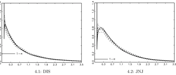
Figure 4 depicts the error densities implied by the quasi maximum likelihood estimates and the semiparametric approach based on the uncorrected gamma kernel. For both stocks, the parametric and semiparametric density are quite close to each other. However, there is a noticeable discrepancy near the mode, which can be explained by the increased bias of the gamma kernel as compared to standard fixed kernels in the interior of the support. To refine the semiparametric density estimate, we employ the
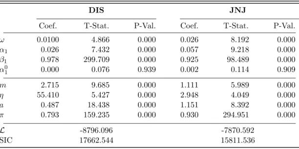
bias-Table 2: Estimation Results – ZA-MEM
Quasi maximum likelihood estimates and t-statistics of the zero-augmented Log-MEM. Lag structure is determined using SIC.
DIS JNJ
Coef. T-Stat. P-Val. Coef. T-Stat. P-Val.
ω 0.0100 4.866 0.000 0.026 8.192 0.000 α1 0.026 7.432 0.000 0.057 9.218 0.000 β1 0.978 299.709 0.000 0.925 98.489 0.000 α01 0.000 0.076 0.939 0.002 0.114 0.909 m 2.715 9.685 0.000 1.111 5.989 0.000 η 55.410 5.427 0.000 2.948 4.049 0.000 a 0.487 18.438 0.000 1.151 8.392 0.000 π 0.793 159.235 0.000 0.930 294.951 0.000 L -8796.096 -7870.592 SIC 17662.544 15811.536
corrected gamma kernel estimator (11), choosing the ZAF distribution as parametric start. The plots in Figure 5 show that, in both cases, the discrepancy near the mode vanishes, as the parametric density now generally lies within the 95%-confidence region of the semiparametric estimate.
The estimation results suggest that the ZAF distribution provides a superior way to model MEM disturbances for cumulated volumes. This graphical intuition can be formally assessed by the proposed semiparametric specification test (14). In the MEM setting (16), we obtain applicable finite sample p-values via the following bootstrap procedure:
Step 1: Draw a random sample {ε∗t}nt=1 from the parametric ZAF distribution with density fε ε,ϑb
, where ϑbis the maximum likelihood estimate of the ZAF parametersϑ
as in (8) from the original data. From this, generate the bootstrap sample {yt∗}nt=1 as
yt∗ = ˆµtε∗t, where ˆµt is the fitted conditional mean as in (17) based on the maximum
likelihood estimates from the original data.
Step 2: Use {yt∗}nt=1 to compute the statistic Tn, which we denote asTn∗. This requires
the re-evaluation of both the parametric and semiparametric estimates of fε(ε).
Step 3: Steps 1 and 2 are repeated B times and critical values are obtained from the empirical distribution of
Tn,r∗ B
r=1.
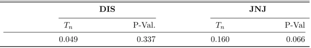
Table 3 displays the test results based onB = 500 bootstrap replications for the critical values. In both cases, the statistic is insignificant at the 5%-level, which implies that we cannot reject the null hypothesis as given in (13). These results confirm that the
4.1: DIS 4.2: JNJ
Figure 4: Estimates of Error Density with Gamma KDE
The black solid line represents the error density implied by the QML estimates of the ZA-MEM. The black dashed line is the semiparametric estimate based on the gamma kernel estimator. The grey dashed lines are 95% confidence bounds of the kernel density estimator. LSCV bandwidths: 0.0212 (DIS), 0.0210 (JNJ). Estimates of 1−π based on sample percentage of zeros values: 0.2068 (DIS), 0.0705 (JNJ).
5.1: DIS 5.2: JNJ
Figure 5: Estimates of Error Density with Corrected Gamma KDE
The black solid line represents the error density implied by the QML-estimates of the ZA-MEM. The black dashed line is the semiparametric estimate based on the bias-corrected gamma kernel estimator. The grey dashed lines are 95% confidence bounds of the kernel density estimator. LSCV bandwidths: 1.3055 (DIS), 1.3067 (JNJ). Estimates of 1−πbased on sample percentage of zeros values: 0.2068 (DIS), 0.0705 (JNJ).
ZA-MEM is able to capture the distributional properties of high-frequency cumulated volumes.
3
Dynamic Zero-Augmented Multiplicative Error Models
3.1 Motivation
Assumption (1) implies that, conditional on past information, the trading probability is constant or, more formally,
π :=P(εt>0|Ft−1) =P(yt>0|Ft−1) =P(It= 1|Ft−1), (19)
whereItis a “trade indicator” taking the value 1 foryt>0 and 0 else. Given that
(non-zero) cumulative volume is clearly time-varying and reveals persistent serial dependencies, the assumption of constant no-trade probabilities appears to be rather restrictive. Moreover, it is at odds with the well-known empirical evidence of autocorrelated trading intensities, see, e.g., Engle and Russell(1998). Table 4 shows the results of a simple runs test based on the trade indicatorIt suggesting that the null hypothesis of no serial
correlation in no-trade probabilities is clearly rejected. Consequently, we propose an augmented version of ZA-MEM accounting also for dynamics in zero occurrences.
3.2 A ZA-MEM with Dynamic Zero Probabilities
Assume that, given the past information set Ft−1, the conditional probability of the
disturbanceεtbeing zero depends on a restricted information setHt−1 ⊂ Ft−1. Moreover,
πt is assumed to depend onHt−1 by a functionπ(·;ψ) with parameter vectorψ,
πt:=P(εt>0|Ft−1) =P(εt>0|Ht−1) =π(Ht−1;ψ). (20)
Table 3: Semiparametric Test for Specification of Error Density
Results of the semiparametric specification test from Section2.3applied to the MEM errorsεt.
The reported p-values are based on the empirical distribution of the test statistic resulting from 500 simulated bootstrap samples.
DIS JNJ
Tn P-Val. Tn P-Val
Table 4: Runs Test for Trade Indicator
Results of the two-sided runs test for serial dependence of the indicator for nonzero aggregated volumes. Under the null of no serial dependence, the statisticZ= R−V(ER(R)) (R: number of runs) is asymptotically standard normal.
DIS JNJ
Z P-Val. Z P-Val
-6.523 0.000 -6.432 0.000
As a consequence of this assumption, the disturbances lose the i.i.d. property and, conditionally on Ht−1, are independently but not identically distributed. Thus, the
dynamics of the endogenous variable,yt, are not fully captured by the conditional mean
µt, as past information contained inHt−1 affects the innovation distribution. Similar
generalizations of the MEM error structure have been considered, e.g., by Zhang et al. (2001) or Drost and Werker (2004). The resulting dynamic zero-augmented MEM (DZA-MEM) can be formally written as
yt=µtεt; εt|Ht−1∼i.n.i.d.PMD(1), (21)
where PMD(1) denotes a point-mass mixture as in (2) with assumption (1) replaced by (20) andE[εt|Ht−1] =E[εt] = 1. Hence, the conditional density ofεt givenHt−1 is
fε(εt|Ht−1) = (1−πt)δ(εt) +πtgε(εt|Ht−1) 1I(εt>0), (22)
where the conditional density for εt >0, gε(εt|Ht−1), depends on Ht−1 through the
probability πt, as the unit mean assumption in (21) requires
κt:=E[εt|εt>0;Ht−1] =π−t1, (23)
such that
E[εt] =E{E[εt|Ht−1]}=E[πtκt] = 1. (24)
Since the functionπ(·;ψ) is equivalent to a binary-choice specification for the trade indicator It defined in (19), the log-likelihood of the DZA-MEM consists of a MEM
and a binary-choice part, L(ϑ) = n X t=1 {It lnπt+ (1− It) ln (1−πt)}+ X t,nz {lnfε(yt/µt|Ht−1;ϑg)−lnµt}, (25)
whereϑ= (ψ, ϑg, ϑµ)0 withϑµ denoting the parameter vector of the conditional mean
µt. As in the previous section, a separate optimization of the two parts is infeasible,
since the constraint (23) implies that both components depend on the parameters of the binary-choice specification,ψ.
If we use the ZAF distribution as point-mass mixture PMD(1), we obtain the conditional density of εtgiven Ht−1 as
fε(εt|Ht−1) = (1−πt)δ(εt) +πt
a εa mt −1[η+ (εtπtξ)a](−η−m)ηη
(πtξ)−a m B(m, η)
1I(εt>0), (26)
where we setλt= (πtξ)−1, withξ defined as in (18), to meet the constraint (23). The
corresponding log-likelihood function is
L(ϑ) = n X t=1 {It lnπt+ (1− It) ln (1−πt)}+ X t,nz loga+ (am−1) lnxt (27) −(η+m) ln η+ xt µt πtξ a +η lnη−amln µtπt−1ξ−1 −lnB(m, η) , whereϑ= (ψ, a, m, η, ϑµ)0.
3.3 Dynamic Models for the Trade Indicator
To allow the trade indicatorItto follow a dynamic process, we propose two alternative
specifications: a parsimonious autologistic specification and a more flexible parameteri-zation using autoregressive conditional multinomial (ACM) dynamics as proposed by Russell and Engle (2005). By considering the general logistic link function
πt=π(Ht−1;ψ) =
exp(ht)
1 + exp(ht)
, (28)
the autologistic specification for ht= ln[πt/(1−πt)] is given by
ht=θ0+ l X i=1 θi∆t−i+gt, andgt= d X i=1 γiIt−i, (29)
where ∆t denotes an indicator for large values of the endogenous variable ofyt and is
defined as
∆t:= max(yt− It,0). (30)
This type of transformation was suggested in a similar setting byRydberg and Shephard (2003) and accounts for the multicollinearity between the lags of yt and It. The
autologistic model has advantages in terms of tractability, such as the concavity of the log-likelihood function, making numerical maximization straightforward. However, since this process does not include a moving average component, it is not able to capture persistent dynamics in the binary sequence. Therefore, as an alternative specification, we propose an ACM specification given by
ht=$+ v X j=1 ρjst−j + w X j=1 ζjht−j, (31) where st−j = It−j−πt−j p πt−j(1−πt−j) (32)
denotes the standardized trade indicator. The process {st} is a martingale difference
sequence with zero mean and unit conditional variance, which implies that {ht} follows
an ARMA process driven by a weak white noise term. Consequently, {ht}is stationary
if all values of z satisfying 1−ζ1z−. . .−ζwzw = 0 lie outside the unit circle. For more
details, see Russell and Engle (2005).
An appealing feature of the ACM specification in the given framework is its sim-ilarity to a MEM. Actually, analogously to a MEM specification, it imposes a linear autoregressive structure for the logistic transformation of the probability πt, which,
in turn, equals the conditional mean of the trade indicator It given the restricted information set Ht−1, i.e., E[It|Ht−1].
The DZA-MEM dynamics can be straightforwardly extended by covariates which allow to test specific market microstructure hypotheses. Moreover, a further natural extension of the DZA-MEM is to allow for dynamic interaction effects between the conditional mean of yt, µt, and the probability of zero values, πt. For instance, by
as ht=$+ v X j=1 ρjst−j+ w X j=1 ζjht−j+ m X j=1 τjµt−j, (33) lnµt=ω+ p X i=1 αi lnεt−i1I(xt−i>0)+ p X i=1 α0i1I(xt−i=0)+ q X i=1 βi lnµt−i+ n X i=1 %iπt−i.
In the resulting model, the intercepts $ and ω are not identified without additional restrictions. Hence, identification requires, for instance, $ = 0. Alternatively, or additionally, dynamic spillover effects might be also modeled by the inclusion of the lagged endogenous variables of the two equations, see, e.g., Russell and Engle(2005) in an ACD-ACM context.
3.4 Diagnostics
The evaluation of the DZA-MEM is complicated by the fact that the disturbances are not i.i.d. In particular, the non-identical distribution makes an application of the semiparametric specification test from Section 2.3 impossible. Moreover, since the disturbances are not i.i.d. even given the restricted information set Ht−1, we cannot
employ a transformation that provides standardized i.i.d. innovations as in De Luca and Zuccolotto (2006). As an alternative, we suggest evaluating the model based on density forecasts as developed by Diebold et al. (1998) and firstly applied to MEM-type models by Bauwens et al. (2004). One difficulty is that this method is designed for continuous random variables, while we have to deal with a discrete probability mass at zero. Therefore, following Liesenfeld et al. (2006) andBrockwell(2007), we employ a modified version of the test. The idea is to add random noise to the discrete component, making sure that the c.d.f. is invertible. Thus, we compute randomized probability integral transforms zt= ( UtFY(yt|Ft−1) ifyt= 0, FY(yt|Ft−1) ifyt>0, (34)
whereFY(yt|Ft−1) denotes the conditional c.d.f. of yt implied by the DZA-MEM, while
Ut are random variables with {Ut}tn=1 being i.i.d. U(0,1). Using equation (22), we
obtain zt= ( Ut (1−πt) ifyt= 0, (1−πt) +πtGε(yt/µt|Ht−1) ifyt>0, (35)
whereGε(yt/µt|Ht−1) is the conditional c.d.f. of the disturbancesεtforεt>0 evaluated
atyt/µt. For a DZA-MEM based on the ZAF distribution, it follows that
zt= ( Ut (1−πt) ifyt= 0, (1−πt) +πt [B(c;m, η)/B(m, η)] ifyt>0, (36) whereB(c;m, η) :=Rc 0 t
m−1(1−t)η−1dt is the incomplete beta function evaluated at
c:= ytµ−t1πtξ ah
η+ ytµ−t1πtξ ai−1
. (37)
If the conditional distribution of yt is correct, the zt sequence is i.i.d. U(0,1), see
Brockwell (2007) for a proof. WhileDiebold et al.(1998) recommend a visual inspection of the properties of the zt’s, we also check for uniformity using Pearson’sχ2-test.
3.5 Empirical Evidence on DZA-MEM Processes
We apply a DZA-MEM by parameterizing the conditional mean functionµt based on
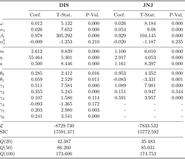
the Log-MEM specification (17). The lag orders in both dynamic components are chosen according to the Schwarz information criterion. Table 5 shows the estimation results for the DZA-MEM with autologistic binary-choice component. No consistent effects for the large volume indicatormtacross the two stocks are found. Large volumes
increase the trading probability in the case of DIS, while reducing it for JNJ. However, the lagged trade indicators are significantly positive in almost every case. Thus, trade occurrences are positively autocorrelated, which is in line with empirical studies on market microstructure (see, e.g., Engle,2000).
For both stocks, all Q-statistics of the autologistic residuals
ut= It−πˆt p ˆ πt (1−πˆt) (38)
are significant at the 5% level, showing that an autologistic specification does not completely capture the dynamics and is too parsimonious.
As shown by Table 6, dynamically modeling trade occurrences by an ACM specifi-cation yields significantly lower Q-statistics. Hence, the ACM specifispecifi-cation seems to fully capture the persistence in the trade indicator series, with the parameter estimates underlining the strong persistence in the process. Actually, the coefficient ζ1 is close to
unity for both stocks suggesting that the underlying process is very persistent.
We evaluate the model using the density forecast approach discussed in Section3.4. Table 7shows the results of the χ2-test for uniformity of the randomized probability
Table 5: Estimation Results – DZA-MEM with Autologistic Component
Maximum likelihood estimates of the DZA-MEM based on the ZAF distribution with autologistic specification for the binary choice component. The Q-statistics refer to the residuals of the autologistic component. 5% critical values of the Q-statistics with 20, 50 and 100 lags are 31.410, 67.505 and 124.342, respectively. The autologistic residuals are defined as:
ut= √It−πˆt
ˆ
πt(1−πˆt)
.
DIS JNJ
Coef. T-Stat. P-Val. Coef. T-Stat. P-Val.
ω 0.012 5.132 0.000 0.026 8.184 0.000 α1 0.026 7.652 0.000 0.054 9.08 0.000 β1 0.978 305.292 0.000 0.929 104.145 0.000 α01 -0.009 -1.253 0.210 -0.020 -1.187 0.235 m 2.612 9.839 0.000 1.100 6.010 0.000 η 55.464 5.301 0.000 2.917 4.053 0.000 a 0.500 8.446 0.000 1.161 8.397 0.000 θ0 0.285 2.412 0.016 0.953 4.352 0.000 θ1 0.059 2.529 0.011 -0.083 -3.331 0.001 γ1 0.511 7.584 0.000 1.089 7.981 0.000 γ2 0.355 5.245 0.000 0.151 0.947 0.344 γ3 0.107 1.580 0.114 0.591 3.957 0.000 γ4 -0.093 -1.365 0.172 - - -γ5 0.203 2.980 0.003 - - -γ6 0.241 3.541 0.000 - - -L -8729.730 -7833.532 SIC 17591.371 15772.592 Q(20) 42.387 35.483 Q(50) 86.260 85.031 Q(100) 173.606 174.753
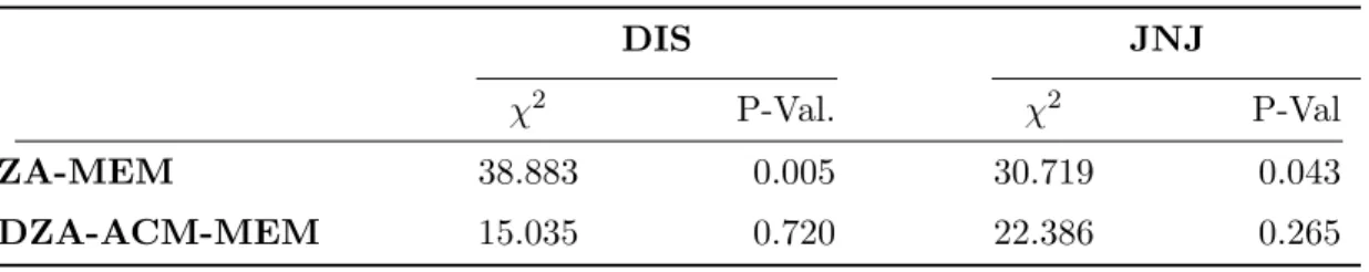
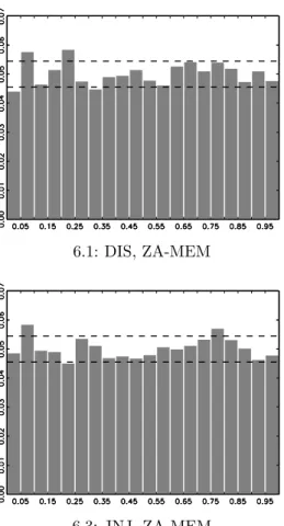
integral transforms (PITs) implied by the ZA-MEM and the DZA-ACM-MEM. For the former specification, the χ2-statistics are significant at the 5% level. In the case of the DZA-ACM-MEM, the null hypothesis of a uniform distribution cannot be rejected at any conventional significance level for both stocks. For DIS, the χ2-statistic nearly halves indicating an impressive performance improvement. These findings are underlined by the histograms of the PITs depicted in Figure6. For both stocks, the PIT histogram implied by the DZA-ACM-MEM is close to a uniform distribution, while almost none of the bars is outside the 95% confidence region.
Table 6: Estimation Results – DZA-MEM with ACM Component
Maximum likelihood estimates of the DZA-MEM based on the ZAF distribution with ACM specification for the binary choice component. The Q-statistics refer to the residuals of the ACM component. 5% critical values of the Q-statistics with 20, 50 and 100 lags are 31.410, 67.505 and 124.342, respectively. The ACM residuals are defined as:
ut= √It−πˆt
ˆ
πt(1−πˆt)
.
DIS JNJ
Coef. T-Stat. P-Val. Coef. T-Stat. P-Val.
ω 0.013 5.721 0.000 0.026 8.374 0.000 α1 0.025 7.780 0.000 0.054 8.987 0.000 β1 0.979 327.030 0.000 0.930 104.084 0.000 α01 -0.018 -2.588 0.010 -0.031 -1.825 0.068 m 2.652 9.493 0.000 1.109 6.555 0.000 η 55.332 4.121 0.000 2.949 4.398 0.000 a 0.495 17.256 0.000 1.152 9.176 0.000 $ 0.023 1.970 0.049 0.112 2.056 0.040 ρ1 0.202 7.820 0.000 0.237 6.940 0.000 ρ2 -0.138 -4.870 0.000 -0.146 -3.815 0.000 ζ1 0.983 116.111 0.000 0.957 45.964 0.000 L -8726.831 -7838.810 SIC 17550.398 15774.355 Q(20) 30.672 20.425 Q(50) 52.548 51.552 Q(100) 109.633 124.276
Table 7: χ2-Test for Uniformity of the PITs
Results of theχ2-test for uniformity of the randomized probability integral transforms of the estimated ZA-MEM and DZA-ACM-MEM specifications.
DIS JNJ
χ2 P-Val. χ2 P-Val
ZA-MEM 38.883 0.005 30.719 0.043
6.1: DIS, ZA-MEM 6.2: DIS , DZA-ACM-MEM
6.3: JNJ, ZA-MEM 6.4: JNJ, DZA-ACM-MEM
Figure 6: Histograms of Computed PIT-Sequences
Histograms of the randomized probability integral transforms of the estimated ZA-MEM and DZA-ACM-MEM specifications. The dashed lines represent 95% confidence bounds.
4
Conclusions
We introduce a new approach for modeling autoregressive positive-valued variables with excess zero outcomes. These properties are typical for both irregularly-spaced and time-aggregated financial high-frequency data and cannot be appropriately handled in extant approaches.
To capture the clustering of observations at zero, we propose a new point-mass mixture distribution, which consists of a discrete component at zero and a flexible continuous distribution for the strictly positive part of the support. To evaluate such a distribution, a novel semiparametric specification test tailored for point-mass mixture distributions is introduced. Finally, to accommodate serial dependencies in the data we incorporate the proposed point-mass mixture into a new type of multiplicative error model (MEM) capturing the dynamics of both zero occurrences and strictly positive values.
The empirical evidence based on cumulated trading volumes of two NYSE stocks shows that a zero-augmented MEM relying on the proposed point-mass mixture is able to capture the occurrence of excess zeros very well. The best fit is shown for a specification incorporating a two-state ACM component for the trade indicator. Besides MEM dynamics in the volumes, the model also explains the (own-standing) dynamics in trade occurrences and produces good density forecasts.
The model is sufficiently flexible to be extended in various ways, e.g., to allow for dynamic spillovers between the two types of dynamics or to incorporate regressors. Moreover, the model is straightforwardly extended to a multivariate framework, in the spirit of, e.g.Manganelli (2005),Cipollini et al. (2006) or Hautsch(2008).
Finally, the proposed ZAF distribution, its dynamic inclusion and the new semi-parametric test for point-mass mixtures could be relevant also in other areas, such as hydrology or genetics (see, e.g., Weglarczyk et al.,2005;Taylor and Pollard,2009).
References
Allen, D., F. Chan, M. McAleer, and S. Peiris (2008): “Finite sample properties
of the QMLE for the Log-ACD model: application to Australian stocks,”Journal of Econometrics, 147, 163–185.
Bauwens, L., F. Galli, and P. Giot (2003): “The moments of Log-ACD models,” CORE Discussion Paper.
Bauwens, L. and P. Giot (2000): “The logarithmic ACD model: an application
to the bid-ask quote process of three NYSE stocks,” Annales D’Economie et de Statistique, 60, 117–149.
Bauwens, L., P. Giot, J. Grammig, and D. Veredas(2004): “A comparison of
financial duration models via density forecasts,”International Journal of Forecasting, 20, 589–609.
Bauwens, L. and N. Hautsch (2008): “Modeling financial high-frequency data with
point processes,” inHandbook of Financial Time Series, ed. by T. G. Andersen, R. A. Davis, J.-P. Kreiss, and T. Mikosch.
Brockwell, A. (2007): “Universal residuals: a multivariate transformation,” Stat
Probab Lett., 77, 1473–1478.
Brownlees, C. T., F. Cipollini, and G. M. Gallo(2010): “Intra-daily volume
modeling and prediction for algorithmic trading,”Journal of Financial Econometrics, 8, 1–30.
Chen, S. (2000): “Probability density function estimation using gamma kernels,”
Cheng, M., J. Fan, and J. Marron(1997): “On automatic boundary corrections,”
The Annals of Statistics, 25, 1691–1708.
Cipollini, F., R. F. Engle, and G. M. Gallo (2006): “Vector multiplicative error
models: representation and inference,” NYU Working Paper No. Fin-07-048.
De Luca, G. and G. M. Gallo (2004): “Mixture Processes for Financial Intradaily
Durations,”Studies in Nonlinear Dynamics & Econometrics, 8.
De Luca, G. and P. Zuccolotto (2006): “Regime-switching pareto distributions
for ACD models,”Computational Statistics & Data Analysis, 51, 2179–2191.
Diebold, F. X., T. A. Gunther, and A. S. Tay (1998): “Evaluating density
forecasts with application to financial risk management,” International Economic Review, 39, 863–883.
Drost, F. C. and B. J. M. Werker (2004): “Semiparametric duration models,”
Journal of Business and Economic Statistics, 22, 40–50.
Duan, N. J., W. G. Manning, C. N. Morris, and J. P. Newhouse (1983):
“A comparison of alternative models for the demand for medical care,” Journal of Business and Economic Statistics, 1, 115–126.
Easley, D. and M. O’Hara (1992): “Time and the process of security price
adjust-ment,”Journal of Finance, 47, 577–605.
Engle, R. F. (2000): “The econometrics of ultra-high-frequency-data,”Econometrica,
68, 1–22.
——— (2002): “New frontiers for ARCH models,” Journal of Applied Econometrics, 17, 425–446.
Engle, R. F. and G. M. Gallo (2006): “A multiple indicators model for volatility using intra-daily data,” Journal of Econometrics, 131, 3–27.
Engle, R. F. and J. Russell (1998): “Autoregressive conditional duration: a new
model for irregularly spaced transaction data,” Econometrica, 66, 1127–1162.
Fan, Y. (1994): “Testting the goodness of of fit of a parametric density function by
kernel method,”Econometric Theory, 10, 316–356.
——— (1998): “Goodness-of-fit tests based on kernel density estimators with fixed smoothing parameters,”Econometric Theory, 14, 604–621.
Fernandes, M. and J. Grammig (2005): “Nonparametric specification tests for
conditional duration models,” Journal of Econometrics, 127, 35–68.
Fernandes, M. and P. Monteiro (2005): “Central limit theorem for asymmmetric
kernel functionals,”Annals of the Institute of Statistical Mathematics, 57, 425–442.
Gasser, T. and H. M¨uller (1979): “Kernel estimation of regression functions,” in
Hagmann, M. and O. Scaillet (2007): “Local multiplicative bias correction for
asymmetric kernel density estimators,”Journal of Econometrics, 141, 213–249.
Hautsch, N. (2003): “Assessing the Risk of Liquidity Suppliers on the Basis of Excess
Demand Intensities,”Journal of Financial Econometrics, 1, 189–215.
——— (2004): Modelling Irregularly Spaced Financial Data: Theory and Practice of Dynamic Duration Models, Berlin: Springer.
——— (2008): “Capturing common components in high-frequency financial time series: A multivariate stochastic multiplicative error model,”Journal of Economic Dynamics & Control, 32, 3978–4009.
Hjort, N. L. and I. K. Glad (1995): “Nonparametric density estimation with a
parametric start,” The Annals of Statistics, 23, 882–904.
Johnson, N. L., S. Kotz, and N. Balakrishnan(1994): Continuous Univariate
Distributions, Volumes I and II, New York: John Wiley and Sons, second ed.
Jones, M.(1993): “Simple boundary correction for kernel density estimation,”Statistics
and Computing, 3, 135–146.
Lancaster, T. (1997): The Econometric Analysis of Transition Data, Cambridge:
Cambridge University Press.
Lanne, M. (2006): “A mixture multiplicative error model for realized volatility,”
Journal of Financial Econometrics, 4, 594–616.
Liesenfeld, R., I. Nolte, and W. Pohlmeier (2006): “Modeling financial
transac-tion price movements: a dynamic integer count model,” Empirical Economics, 30, 795–825.
Manganelli, S.(2005): “Duration, Volume and volatility impact of trades,” Journal
of Financial Markets, 8, 377–399.
Russell, J. R. and R. F. Engle (2005): “A discrete-state continuous-time model of
financial transactions prices and times: the autoregressive conditional multinomial-autoregressive conditional duration model,”Journal of Business & Economic Statis-tics, 23, 166–180.
Rydberg, T. and N. Shephard(2003): “Dynamics of trade-by-trade price movements:
decomposition and models,”Journal of Financial Econometrics, 1, 2–25.
Schuster, E.(1958): “Incorporating support constraints into nonparametric estimators of densities,”Communications in Statistics, Part A - Theory and Methods, 14, 1123– 1136.
Taylor, S. and K. Pollard (2009): “Hypothesis tests for point-mass mixture data
with application to omics data with many zero values,” Statistical Applications in Genetics and Molecular Biology, 8, 1–43.
Weglarczyk, S., W. G. Stupczewski, and V. P. Singh (2005): “Three parameter
discontinuous distributions for hydrological samples with zero values,”Hydrological Processes, 19, 2899–2914.
Zhang, M. Y., J. R. Russell, and R. S. Tsay (2001): “A nonlinear autoregressive
conditional duration model with applications to financial transaction data,”Journal of Econometrics, 104, 179–207.
Zhang, S. (2010): “A note on the performance of gamma kernel estimators at the
SFB 649 Discussion Paper Series 2010
For a complete list of Discussion Papers published by the SFB 649,
please visit http://sfb649.wiwi.hu-berlin.de.
001 "Volatility Investing with Variance Swaps" by Wolfgang Karl Härdle and Elena Silyakova, January 2010.
002 "Partial Linear Quantile Regression and Bootstrap Confidence Bands" by Wolfgang Karl Härdle, Ya’acov Ritov and Song Song, January 2010. 003 "Uniform confidence bands for pricing kernels" by Wolfgang Karl Härdle,
Yarema Okhrin and Weining Wang, January 2010.
004 "Bayesian Inference in a Stochastic Volatility Nelson-Siegel Model" by Nikolaus Hautsch and Fuyu Yang, January 2010.
005 "The Impact of Macroeconomic News on Quote Adjustments, Noise, and Informational Volatility" by Nikolaus Hautsch, Dieter Hess and David Veredas, January 2010.
006 "Bayesian Estimation and Model Selection in the Generalised Stochastic Unit Root Model" by Fuyu Yang and Roberto Leon-Gonzalez, January 2010.
007 "Two-sided Certification: The market for Rating Agencies" by Erik R.
Fasten and Dirk Hofmann, January 2010.
008 "Characterising Equilibrium Selection in Global Games with Strategic Complementarities" by Christian Basteck, Tijmen R. Daniels and Frank Heinemann, January 2010.
009 "Predicting extreme VaR: Nonparametric quantile regression with refinements from extreme value theory" by Julia Schaumburg, February 2010.
010 "On Securitization, Market Completion and Equilibrium Risk Transfer" by Ulrich Horst, Traian A. Pirvu and Gonçalo Dos Reis, February 2010.
011 "Illiquidity and Derivative Valuation" by Ulrich Horst and Felix Naujokat,
February 2010.
012 "Dynamic Systems of Social Interactions" by Ulrich Horst, February 2010.
013 "The dynamics of hourly electricity prices" by Wolfgang Karl Härdle and Stefan Trück, February 2010.
014 "Crisis? What Crisis? Currency vs. Banking in the Financial Crisis of 1931" by Albrecht Ritschl and Samad Sarferaz, February 2010.
015 "Estimation of the characteristics of a Lévy process observed at arbitrary frequency" by Johanna Kappusl and Markus Reiß, February 2010.
016 "Honey, I’ll Be Working Late Tonight. The Effect of Individual Work Routines on Leisure Time Synchronization of Couples" by Juliane Scheffel, February 2010.
017 "The Impact of ICT Investments on the Relative Demand for High-Medium-, and Low-Skilled Workers: Industry versus Country Analysis" by Dorothee Schneider, February 2010.
018 "Time varying Hierarchical Archimedean Copulae" by Wolfgang Karl Härdle, Ostap Okhrin and Yarema Okhrin, February 2010.
019 "Monetary Transmission Right from the Start: The (Dis)Connection Between the Money Market and the ECB’s Main Refinancing Rates" by Puriya Abbassi and Dieter Nautz, March 2010.
020 "Aggregate Hazard Function in Price-Setting: A Bayesian Analysis Using Macro Data" by Fang Yao, March 2010.
021 "Nonparametric Estimation of Risk-Neutral Densities" by Maria Grith, Wolfgang Karl Härdle and Melanie Schienle, March 2010.
022 "Fitting high-dimensional Copulae to Data" by Ostap Okhrin, April 2010. 023 "The (In)stability of Money Demand in the Euro Area: Lessons from a
Cross-Country Analysis" by Dieter Nautz and Ulrike Rondorf, April 2010. 024 "The optimal industry structure in a vertically related market" by
Raffaele Fiocco, April 2010.
025 "Herding of Institutional Traders" by Stephanie Kremer, April 2010.
026 "Non-Gaussian Component Analysis: New Ideas, New Proofs, New Applications" by Vladimir Panov, May 2010.
027 "Liquidity and Capital Requirements and the Probability of Bank Failure" by Philipp Johann König, May 2010.
028 "Social Relationships and Trust" by Christine Binzel and Dietmar Fehr, May 2010.
029 "Adaptive Interest Rate Modelling" by Mengmeng Guo and Wolfgang Karl
Härdle, May 2010.
030 "Can the New Keynesian Phillips Curve Explain Inflation Gap Persistence?" by Fang Yao, June 2010.
031 "Modeling Asset Prices" by James E. Gentle and Wolfgang Karl Härdle, June 2010.
032 "Learning Machines Supporting Bankruptcy Prediction" by Wolfgang Karl Härdle, Rouslan Moro and Linda Hoffmann, June 2010.
033 "Sensitivity of risk measures with respect to the normal approximation
of total claim distributions" by Volker Krätschmer and Henryk Zähle, June 2010.
034 "Sociodemographic, Economic, and Psychological Drivers of the Demand for Life Insurance: Evidence from the German Retirement Income Act" by Carolin Hecht and Katja Hanewald, July 2010.
035 "Efficiency and Equilibria in Games of Optimal Derivative Design" by Ulrich Horst and Santiago Moreno-Bromberg, July 2010.
036 "Why Do Financial Market Experts Misperceive Future Monetary Policy Decisions?" by Sandra Schmidt and Dieter Nautz, July 2010.
037 "Dynamical systems forced by shot noise as a new paradigm in the interest rate modeling" by Alexander L. Baranovski, July 2010.
038 "Pre-Averaging Based Estimation of Quadratic Variation in the Presence of Noise and Jumps: Theory, Implementation, and Empirical Evidence" by Nikolaus Hautsch and Mark Podolskij, July 2010.
039 "High Dimensional Nonstationary Time Series Modelling with Generalized
Dynamic Semiparametric Factor Model" by Song Song, Wolfgang K. Härdle, and Ya'acov Ritov, July 2010.
040 "Stochastic Mortality, Subjective Survival Expectations, and Individual
Saving Behavior" by Thomas Post and Katja Hanewald, July 2010.
041 "Prognose mit nichtparametrischen Verfahren" by Wolfgang Karl Härdle, Rainer Schulz, and Weining Wang, August 2010.
042 "Payroll Taxes, Social Insurance and Business Cycles" by Michael C. Burda and Mark Weder, August 2010.
043 "Meteorological forecasts and the pricing of weather derivatives" by Matthias Ritter, Oliver Mußhoff, and Martin Odening, September 2010. 044 "The High Sensitivity of Employment to Agency Costs: The Relevance of
Wage Rigidity" by Atanas Hristov, September 2010.
045 "Parametric estimation of risk neutral density functions" by Maria Grith and Volker Krätschmer, September 2010.
SFB 649 Discussion Paper Series 2010
For a complete list of Discussion Papers published by the SFB 649,
please visit http://sfb649.wiwi.hu-berlin.de.
046 "Mandatory IFRS adoption and accounting comparability" by Stefano Cascino and Joachim Gassen, October 2010.
047 "FX Smile in the Heston Model" by Agnieszka Janek, Tino Kluge, Rafał
Weron, and Uwe Wystup, October 2010.
048 "Building Loss Models" by Krzysztof Burnecki, Joanna Janczura, and
Rafał Weron, October 2010.
049 "Models for Heavy-tailed Asset Returns" by Szymon Borak, Adam
Misiorek, and Rafał Weron, October 2010.
050 "Estimation of the signal subspace without estimation of the inverse covariance matrix" by Vladimir Panov, October 2010.
051 "Executive Compensation Regulation and the Dynamics of the Pay-Performance Sensitivity" by Ralf Sabiwalsky, October 2010.
052 "Central limit theorems for law-invariant coherent risk measures" by Denis Belomestny and Volker Krätschmer, October 2010.
053 "Systemic Weather Risk and Crop Insurance: The Case of China" by Wei
Xu, Ostap Okhrin, Martin Odening, and Ji Cao, October 2010.
054 "Spatial Dependencies in German Matching Functions" by Franziska Schulze, November 2010.
055 "Capturing the Zero: A New Class of Zero-Augmented Distributions and Multiplicative Error Processes" by Nikolaus Hautsch, Peter Malec and Melanie Schienle, November 2010.