Computational Study of Free Jets Emanating from Circular and Lobed Orifice-Lattice Boltzmann Method

Lehigh University

Lehigh Preserve

Theses and Dissertations

8-1-2018

Computational Study of Free Jets Emanating from

Circular and Lobed Orifice-Lattice Boltzmann

Method

Yang Chen

Lehigh University, [email protected]

Follow this and additional works at:https://preserve.lehigh.edu/etd

Part of theMechanical Engineering Commons

This Dissertation is brought to you for free and open access by Lehigh Preserve. It has been accepted for inclusion in Theses and Dissertations by an authorized administrator of Lehigh Preserve. For more information, please [email protected].

Recommended Citation

Chen, Yang, "Computational Study of Free Jets Emanating from Circular and Lobed Orifice-Lattice Boltzmann Method" (2018).

Theses and Dissertations. 4269. https://preserve.lehigh.edu/etd/4269

Computational Study of Free Jets Emanating from

Circular and Lobed Orifice-Lattice Boltzmann

Method

by

Yang Chen

A Dissertation

Presented to the Graduate and Research Committee of Lehigh University

in Candidacy for the Degree of Doctor of Philosophy

in

Mechanical Engineering

Lehigh University August 2018

ii

© 2018 Copyright Yang Chen

iii

DISSERTATION SIGNATURE SHEET

Approved and recommended for acceptance as a dissertation in partial fulfillment of the requirements for the degree of Doctor of Philosophy.

______________________ Date ______________________ Dr. Alparslan Oztekin Dissertation Director ______________________ Accepted Date Committee Members: ________________________ Dr. Alparslan Oztekin ________________________ Dr. Yue Yu ________________________ Dr. Edmund Webb III

________________________ Dr. Yaling Liu

iv

ACKNOWLEDGEMENTS

There are many people, whom I would like to acknowledge for their support, suggestions and help. I express extraordinary respect to my great two advisors. I would first like to thank Dr. Alparslan Oztekin and Dr. Yue Yu for their patient guidance, solid support and meticulous help. Alp’s solid background and extreme research experience helped me expand my academic breadth. Yue gave me patient suggestions about Mathematic modeling and coding and helped me significantly on code debugging. I also would like to appreciate Dr. Edmund Webb III and Dr. Yaling Liu for serving as committee members for this dissertation. I also wish to thank Dr. Xiaoyi He, one of the top experts in the field of Lattice Boltzmann Method around the world and my PhD internship supervisor at Air Products & Chemicals.

Through some emotional moments, some great friends I made at Lehigh give me tremendous help not only about the academic research and about mental support. Wei Wei, Haolin Ma, Guosong Zeng, Shengmeng Rong, Weina Wang, Xiao Ma and Jia Liu became good friends, inspiring each other with brilliant ideas, sharing both happiness and sadness and material and spiritual help.

I would also like to thank my parents, Yuangang Chen and Jinchuan Shi, for all their support and love all the time during my whole doctoral journey. They are always my spiritual support.

v

TABLE OF CONTENTS

Mathematical and Numerical Algorithm ... 9

2.1 Single-relaxation time Lattice Boltzmann Method with LES model ... 9

2.2 Multi-block approach in Lattice Boltzmann Method ... 12

2.3 Boundary condition... 14

2.4 Pseudopotential Lattice Boltzmann Method ... 16

2.5 openMPI parallel algorithm ... 19

2.6 Summary ... 21

Single-phase jet from circular and lobed nozzle ... 23

3.1 Introduction ... 23

3.2 Single-phase jet from circular orifice ... 27

3.3 Single-phase jet from 6-lobed orifice ... 56

Multiphase jet flows issued from a circular nozzle ... 76

4.1 Introduction ... 76 4.2 Droplets ... 78 4.3 Simulation setup ... 90 4.4 Results ... 93 4.5 Conclusion ... 102 Conclusion ... 104 5.1 Future work ... 106 References ... 107 Vita ... 111

vi

LIST OF TABLES

Table 1 Uniform exit velocity and actual exit Reynolds Number (built with the

equiseta diameter and the exit velocity) ... 27

Table 2 Inverse of scaled centerline streamwise velocity decay starts location and slope as a function of the Reynolds number ... 43

Table 3 Turbulence plots’ features as a function of the jet Reynolds number ... 46

Table 4 Computational grid size ... 59

Table 5 Uniform exit velocity and actual exit Reynolds Number of 6-lobed jet ... 59

Table 6 Simulation conditions for dimensionless numbers under lattice unit ... 92

Table 7 Surface tension, Weber number and Oh number obtained through Laplace analysis ... 94

Table 8 Physical properties of test fluids ... 98

vii

LIST OF FIGURES

Figure 1 D319 lattice units velocity directions on cube lattice ... 10

Figure 2 Interface structure between two blocks of different lattice spacing ... 12

Figure 3 Lattice nodes of curved boundary ... 15

Figure 4 Schematic of domain decomposition along streamwise direction for openMPI parallel computing algorithm ... 20

Figure 5 Sketch of expected topology of circular free jet ... 23

Figure 6 Schematic representation of jet nozzle exit for circular and 6-lobde case; (a) Diameter of circular orifice exits; (b) equivalent diameter of 6-lobed nozzle exit... 26

Figure 7 boundary conditions for single-phase circular and 6-lobed jet simulation ... 27

Figure 8 Structured mesh shown in XZ plane view ... 29

Figure 9 Flow chat of the computational procedure using multi-block approach ... 32

Figure 10 schematic of refined mesh around circular jet nozzle exit ... 34

Figure 11 Lattice nodes of curved boundary ... 35

Figure 12 Strouhal number versus scaled distance between two circular cylinders at Re=100 ... 37

Figure 13 Instantaneous vorticity contours for the flow past two stationary cylinders in tandem at Re=100 of LBM simulation results: Left is S/D=3.5 case; right is S/D=4.0 case ... 38

Figure 14 Instantaneous vorticity contours for the flow past two stationary cylinders in tandem at Re=100 of reference in Lin 2012: Left is S/D=3.5 case; right is S/D=4.0 case ... 38

Figure 15 The scaled mean centerline streamwise velocity vs the normalized length obtained by two different mesh density at Re=72000 ... 39

Figure 16 Scaled mean centerline streamwise velocity of all different Reynolds number cases ... 40

Figure 17 Comparison of scaled mean centerline streamwise velocity at Re=1050 between LBM simulation and experimental reference [24] ... 41

Figure 18 Comparison of scaled mean centerline streamwise velocity at Re=2700 between LBM simulation and experimental reference [24] ... 42

Figure 19 Comparison of scaled mean centerline streamwise velocity at Re=4050 between LBM simulation and experimental reference [24] ... 42

Figure 20 Inverse of scaled mean centerline streamwise velocity of all Reynolds number cases ... 43

Figure 21 Scaled mean centerline streamwise turbulence intensity of all different Reynolds number cases ... 45

viii

Figure 22 2 seconds spans of velocity signal at X/D = 1, 2, 4, 5, 6 and 10 for Re=2700

... 47

Figure 23 2 seconds spans of velocity signal at X/D = 1, 2, 4, 5, 6 and 10 for Re=1620 ... 47

Figure 24 Normalized power spectra of velocity signals for Re = 2700 ... 49

Figure 25 Normalized power spectra of velocity signals for Re = 4050 ... 50

Figure 26 Flow images, case Re-1050, at 2.0s, 2.5s, 3.378s, 4.563s and 6.25s from top to bottom ... 51

Figure 27 Flow images, case Re=2700, at 1.7s, 1.79s, 1.85s, 2.05s and 2.57s from top to bottom ... 52

Figure 28 Instantaneous vorticity images for different Reynolds number cases ... 54

Figure 29 Schematic representation of 6-lobed nozzle exit ... 58

Figure 30 six-lobed jet orifice geometry and refined mesh around the exit ... 58

Figure 31 Normalized minor plane instantaneous streamwise velocity contours of 6-lobed jet (left) and circular jet (right) for Re=2700 at t=8s ... 61

Figure 32 Comparison of 6-lobed orifice and circular orifice for normalized mean centerline streamwise velocity at Re=2700 case ... 62

Figure 33 Normalized instantaneous streamwise velocity contours of 6-lobed jet in the XZ plane (left) and YZ plane (right) for Re=72000 at t=2s ... 63

Figure 34 Comparison of centerline streamwise mean velocity with Mi 2010 [33] at Re=72000 ... 64

Figure 35 Normalized minor plane instantaneous streamwise velocity contours of 6-lobed jet (left) and circular jet (right) for Re=72000 at t=2s ... 65

Figure 36 Comparison of mean centerline streamwise velocity for 6-lobed and circular jet orifice for Re=72000 case ... 66

Figure 37 Contours of normalized RMS of streamwise velocity fluctuation at major plane of 6-lobed orifice jet (left); minor plane of 6-lobed jet orifice (middle); major plane of circular jet orifice (right) ... 67

Figure 38 Comparison of centerline turbulent kinetic energy with Mi 2010 [33] at Re=72000 ... 69

Figure 39 Instantaneous vorticity contours for Re=72000 case at t=0.006s: (left) circular nozzle exit major plane; (right) 6-lobed nozzle exit minor plane ... 70

Figure 40 Instantaneous flow images of 6-lobed jet at major plane streamwise velocity for Re=72000 case, at (a) 0.0015s; (b) 0.0021s; (c) 0.0051s; (d) 0.0083s; (e) 0.0139s; (f) 0.0255s ... 71

Figure 41 Instantaneous flow images of 6-lobed jet at minor plane streamwise velocity for Re=72000 case, at (a) 0.0015s; (b) 0.0021s; (c) 0.0051s; (d) 0.0083s; (e) 0.0139s; (f) 0.0255s ... 72

ix

Figure 42 Instantaneous flow images of circular jet at minor plane streamwise velocity for Re=72000 case, at (a) 0.0015s; (b) 0.0021s; (c) 0.0051s; (d) 0.0083s; (e)

0.0139s; (f) 0.0255s ... 73

Figure 43 Name definitions for the propose investigation (a) liquid jet and (b) ligament ... 76

Figure 44 Location of simulation parameters on the regime map mentioned ... 77

Figure 45 Comparison of log10 scales density of components along y=100 for oil and air system 900:1 ... 79

Figure 46 Density of Oil contour at t=0.001s, 0.002s, 0.00273s, 0.00283s, 0.0032s and 0.0036s ... 80

Figure 47 Comparison of density of components along centerline (z=30, y=30, 0≤x≤100) ... 82

Figure 48 Normalized components density along centerline (z=30, y=30, 0≤x≤100) at G12=0.2, G21=1.0 ... 83

Figure 49 LBM results of pressure difference versus inverse of droplet radius for static droplet radius ... 84

Figure 50 Simulation results of different equilibrium contact angels for a liquid droplet on a flat and uniform no-slip solid wall with different liquid-solid interaction strength 𝑔𝑤 ... 87

Figure 51 Instantons Iso-surface of Droplets deformation at 𝑔𝑤 = -1.5 ... 88

Figure 52 Instantons Iso-surface of Droplets deformation at 𝑔𝑤 = -2.5 ... 89

Figure 53 boundary conditions for liquid-liquid system circular jet simulation ... 91

Figure 54 Instantaneous flow images of Re=460 case: 𝛾_𝜌 = 1.3, 𝛾_𝜗= 1.4 and We=1.52. The computation domain is set to be 100×100×300. A droplet forms mainly at the tip of jet; the character of varicose breakup (Regimes II) appear. ... 95

Figure 55 Flow images comparison of Re=460 case between pseudopotential LBM simulation and experiment [45] ... 96

Figure 56 Comparison of the present result of Re=460 case in the dimensionless diagram ... 96

Figure 57 Instantaneous Iso-surface flow images of Re=3400 case: 𝛾𝜌 = 1.3, 𝛾𝜗 = 1.4 and We=1 × 104. The computation domain is set to be 240 × 240 × 600. the character of atomization breakup (Regimes IV) appear. ... 101

Figure 58 Reference using color-fluid Lattice Boltzmann Method results of Re=3400, 𝛾_𝜌 = 1.3, 𝛾_𝜗= 1.4, We=1 × 104 and Fr=8.5 case. The computational domain is set to be 240 × 240 × 600. A large number of droplets are entrained from the jet surface; the character of atomization breakup (Regimes IV) appear. ... 101

Figure 59 Summary of the openFOAM simulation result in the dimensionless diagram ... 102

1

ABSTRACT

The Lattice Boltzmann method is an effective computational fluid dynamics tool to study complex flows. Unlike conventional numerical schemes based on discretization of macroscopic continuum equations, the Lattice Boltzmann

method is based on particles and mesoscopic kinetic equations. Single-Relaxation Time Lattice Boltzmann Method (SRTLBM) with Smagorinsky LES model is applied to simulate high Reynolds number jet flows of single and multiphase flows

emanating. The multi-block approach is implemented to refine the mesh when the high resolution is needed in the region around the core jet. An 2nd _order

accurate interface treatment between neighboring blocks is derived to satisfy the conservation of mass momentum and the continuity of the stresses across the interface. The bounce back boundary condition and curve boundary condition using extrapolation approach based on the idea of bounce back of the non-equilibrium part is implemented to impose the velocity boundary conditions at surfaces. The core jet length, velocity decay, turbulence intensity, vortex

generation, jet breakup and noise spectrum analysis are studied for both circular and lobed jet orifices for a range of Reynolds number from 1000 to 72000. The pseudopotential Shan/Chen model Lattice Boltzmann Method is applied to study the small density ratio at low Reynold’s number and low Weber number liquid jet breakup of the water/silicon oil multiphase fluid. Multiphase jet flow simulations at high Reynold’s number and high Weber number are performed by utilizing OpenFOAM and predicted results are compared with results of documented experimental measurements.

2

NOMENCLATURES

Equilibrium distribution function Single-Relaxation time

Lattice directional velocity Collision term

Spatial coordinate Time

Relaxation time Density

Bulk velocity of the fluid Weighting factor

Lattice speed

Differential time operator Speed of sound

Kinematic viscosity Turbulent viscosity Filtered strain rate tensor Smagorinsky constant Reynolds number Time step

Non-equilibrium distribution function Interaction force Gravity acceleration Gas constant Temperature Attractive parameter Repulsion parameter Aspect ratio Equivalent diameter Length of domain Width of domain

3 H St S/D 𝑈∗ Z/D TI f rms 𝑘̅ G P 𝛾_𝜌 𝛾𝜗 𝑊𝑒 𝐹𝑟 𝑂ℎ Height of domain Strouhal number

Normalized distance by diameter of cylinder Normalized velocity

Normalized distance by diameter of jet orifice Turbulence intensity

Frequency in Hz Root-mean square

Turbulence kinetic energy Strength of interaction force Pressure

Density ratio

Kinematic viscosity ratio Weber number Froude number Ohnesorege’s number Subscripts 𝛼 x y z w o Lattice branch x coordinate y coordinate z coordinate water oil Greek’s Symbol ∆ ∇ 𝜓 𝜎 𝜃 Difference Gradient Effective mass Surface tension Contact angle

4

Chapter 1

Introduction

1.1

Motivation

Single and multiphase jets emanating from circular and lobed orifices are encountered in a number of diverse applications. Some of typical applications include air supply for mechanical ventilation in buildings, heat exchangers in industrial processes, aircraft propulsion, etc. Such flows are useful because of their intrinsic properties of providing an efficient mixing by exchanging mass, momentum and/or heat. Liquid-liquid jet flows appear in many natural and industrial processes, e.g., chemical processing and industrial gas storage in oceans. Especially in the nuclear engineering field, the interaction between melt and coolant must be well understood for the safety design of nuclear reactors. Although the air jet and liquid-liquid jets issued from circular and lobed orifices are well studied using

computational and experimental methods, there are still outstanding issues to be addressed Lattice Boltzmann Method can be used to study these flows. Compared with other macroscopic CFD methods based on the Naiver-Stokes equations solvers, Lattice Boltzmann Method focuses on microscopic kinetic equations and offers several advantages. First, the macroscopic mass and momentum is calculated from the discretized distribution functions of each node, which is related to the local neighboring nodes. Second, Lattice Boltzmann Method is easy to be implemented for flow in complex geometries. Third, parallel computing using sub domain with Message Passing Interface approach can be effectively applied to solve Lattice

5

Boltzmann governing equations. Fourth, comparing with VOF method,

pseudopotential Lattice Boltzmann Method for multi-phase flow simulations can dispose phases separations automatically avoiding tracking the fluid phase fracture.

1.2

Literature Review

The Lattice Boltzmann method is widely used to simulate complex flow problems. Unlike conventional numerical schemes based on discretization of macroscopic continuum equations, the Lattice Boltzmann method is based on microscopic models and mesoscopic kinetic equations.

The kinetic nature of the LBM introduces three important features that distinguish it from other numerical methods such as finite element method (FEM) and finite difference method (FDM). First, the convection operator (the streaming process) of the LBM in phase space (velocity space) is linear. This feature is borrowed from the kinetic theory and contrasts with the nonlinear convection terms in other

approaches that use a macroscopic representation. Simple convection combined with a relaxation operator (the collision process) of the LBM allows the recovery of the nonlinear macroscopic advection through multi-scale expansions. Second, the incompressible Naiver-Stokes (NS) equations can be obtained in the nearly

incompressible limit of LBM. The pressure of LBM is calculated by using an equation of state. In contract, in the direct numerical simulation of the incompressible NS equations, the pressure satisfies a Poisson equation with velocity strains acting as sources. Solving this equation for the pressure often produces numerical difficulties, which requires special treatment, such as iteration or relaxation. Third, the LBM utilizes a minimal set of velocities in phase space. Because only one or two speeds and a few directions are used in LBM, the transformation relates to the microscopic

6

distribution function and macroscopic quantities is greatly simplified and required of simple arithmetic calculations. Additionally, most properties in Lattice Boltzmann method are local, which means a large matrix calculation is not needed. For each lattice, mass and momentum are calculated by 9 local discretized distribution populations (or nineteen for three-dimensional model). In addition, Lattice Boltzmann Method can be easily parallelized [1] [2] [3].

In the literature, the lattice Boltzmann equation with the single-relaxation-time (SRT) approximation also known as Bhavnagar-Gross-Krook (BGK) model [4], is the most popular, accurate and efficient scheme. However, the simplicity of the lattice BGK model comes at the expense of numerical instability and inaccuracy in implementing boundary conditions, especially with high Reynolds number flows. These deficiencies in the LBGK models can be overcome with the use of SRT-LES model [5]. In the Smagorinsky model, the sub-grid stress is determined with the strain-rate tensor from the non-equilibrium moments [6].

Several treatments for the curve solid boundary condition are researched, e.g. Guo et al., [7]; Ladd, 1994 [8]; Mei et al., 1999 [9]; He et al. [10]. In the present study of single phase fluid flow, an extrapolation method developed by Guo et al. is adopted for the jet emanating from circular orifice. This treatment has been proved to be of the second order accuracy and has well-behaved stability characteristics.

Considering the simulation efficiency and computational cost, a low-resolution LBM simulation runs on a coarse grid and models global flow behavior of the entire domain with low consumption of computational resources. For regions of inner volume including jet orifice, LBM simulation is performed on fine grids, which are superposed on the coarse one [11]. The global simulation on the coarse grids

7

determines the flow properties on boundaries of the fine grids. Thus, the locally refined fine-grid simulations follow the global fluid behavior and model the desired small-scale and turbulent flow motion with their denser numerical discretization [12]. Besides the performance improvement of the adaptive simulation, the locally refined LBM is suitable for acceleration on parallel computing (openMPI).

The pseudopotential model presented by Shan and Chen in 1993 [13], is the most widely used LBM for multi-phase flow problems. The basic concept is to obtain the microscopic molecular interactions at the mesoscopic scale using an effective mass depending on the local microscopic density. With such interaction forces, the fluid flow separates into two phases with high and low densities when the interaction force strength is modified under critical values. Such automatic phase separation is an attractive character as the phase interface is no longer a mathematical boundary and no explicit interface tracking or capturing is needed [14]. The densities change smoothly from one bulk value to another across the phase interface, which usually occupied several lattice nodes. Due to its computational efficiency, and clear representation of microscopic physics, this pseudopotential model has been successfully applied into a wealth of research fields such as fluid mixing, energy, environment, biology and geology [15].

1.3

Dissertation structure

In this study, we implement the Lattice Boltzmann Method to investigate single-phase and multi-single-phase jet flow issued from circular and lobed jet orifices.

Simulations are conducted for a widely range of Reynolds number. The jet breakup phenomenon and vortex generation shall be studied for the air jet and water/silicon oil liquid-liquid systems. The numerical method is detailed in Chapter 2 with a

8

summary included for the algorithm employed. In Chapter 3, the results of single-phase air jet flows issued from circular and lobed orifices are presented. In Chapter 4, the results of large density ratio droplets and liquid-liquid system jet breakup simulations are presented. Conclusion and outlook for future research and investigations are presented in Chapter 5.

9

Chapter 2

Mathematical Model and Numerical Algorithm

2.1

Single-relaxation time Lattice Boltzmann Method with LES model

In D3Q19 lattice configuration, space is discredited into a cube lattice, and there are 19 discrete velocities. Lattice Boltzmann governing equation yields:

𝑓𝛼(𝑥 + 𝑒𝛼𝛻𝑡, 𝑡 + 𝛻𝑡) − 𝑓𝛼(𝑥, 𝑡) = 𝛺𝛼 (1) 𝑒_𝛼 = { (0,0,0), 𝛼 = 0 (±1,0,0), (0, ±1,0), (0,0, ±1), 𝛼 = 1 − 6 (±1, ±1,0), (±1,0, ±1), (0, ±1, ±1), 𝛼 = 7 − 18 (2)

where 𝑓𝛼(𝑥, 𝑡) is the distribution function at computing node x at time t, and

𝑓𝛼(𝑥 + 𝑒𝛼∇𝑡, 𝑡 + ∇𝑡) is the distribution function after advection and changes due to

Ω_𝛼. Ω_𝛼 satisfies conservation laws and be compatible with the symmetry of the model.

For the single-relaxation time collision term yields

𝛺𝛼 = − 1 𝜏[𝑓𝛼(𝑥, 𝑡) − 𝑓𝛼 𝑒𝑞_{(𝑥, 𝑡)]} (3) where 𝜏 is the dimensionless relaxation time, and 𝑓_𝛼𝑒𝑞(𝑥, 𝑡) is the equilibrium

distribution function defined as:

𝑓_𝛼𝑒𝑞(𝑥, 𝑡) = 𝑤_𝛼𝜌[1 + (3𝑒⃗⃗⃗⃗ ∙𝑢𝛼⃗⃗ 𝑐2 + 9(𝑒⃗⃗⃗⃗ ∙𝑢𝛼⃗⃗ )2 𝑐4 − 3 2 𝑢2 𝑐2)] (4)

10 where 𝜌 is the local density, and 𝑐 = ∇𝑥

∇𝑡 = 1 (in lattice unit). The speed of sound is

𝑐𝑠 = 𝑐/√3. The weighting factors 𝑤𝛼 for the D3Q19 are 𝑤0 = 1 3, 𝑤1−6 = 1 18, 𝑤7−18= 1 36.

Figure 1 D319 lattice units velocity directions on cube lattice

The mass and momentum conservations are strictly enforced

𝜌= ∑18𝛼=0𝑓𝛼 (5)

𝜌𝑢 = ∑18_𝛼=0𝑓_𝛼∙ 𝑒_𝛼 (6)

The hydrodynamic equations derived from above equations via the Chapman-Enskog

analysis are

𝜕_𝑡𝜌 + 𝛻⃗ ∙ 𝜌𝑢⃗ = 0 (7)

𝜕_𝑡𝑢⃗ + 𝑢⃗ ∙ 𝛻⃗ 𝑢⃗ = −𝛻⃗ 𝑝 + 𝜗𝛻2_{𝑢⃗ + 𝑎 (8)}

11 Where 𝑝 = 𝑐_𝑠2_𝜌/𝜌

0 and the kinematic viscosity 𝜗 has the following relation with the relaxation time

𝜗 =1

3(𝜏 −

1

2) (9) The LES method is a powerful tool in numerical simulation of turbulent flows. The

basic idea of LES is based on the following assumptions: the small-scale structures of sub-grid flow field is not sensitive to the large-scale structures of flow field, neither to the influence of boundary conditions. Therefore, small-scale structures are more general, and easier to model [6].

For LES turbulence model, 𝜗_{𝑡𝑜𝑡𝑎𝑙} = ϑ + 𝜗_{𝑒𝑑𝑑𝑦}, where ϑ and 𝜗_{𝑒𝑑𝑑𝑦} are the molecular viscosity and turbulent viscosity (or eddy viscosity), respectively. In the Smagorinsky model, the eddy viscosity 𝜗_{𝑒𝑑𝑑𝑦} is determined with the filtered strain rate tensor

𝑆𝛼𝛽 = (𝜕𝛼𝑢𝛽+ 𝜕𝛽𝑢𝛼)/2, a filter length scale ∆𝑥 and the Smagorinsky constant 𝐶𝑠 [6]:

𝑆_𝑖𝑗 ≈ −3

2𝜌𝑐2_𝜏∆𝑡𝑄𝑖𝑗 (10) where 𝑄_𝑖𝑗 = ∑ 𝑒_{𝛼 𝛼,𝑖}𝑒_𝛼,𝑗(𝑓_𝛼− 𝑓_𝛼𝑒𝑞).

For convenience, we use the notation 𝑓_𝛼 and 𝑆_𝑖𝑗 to denote the filtered variables of the resolved scale in the LBM-LES algorithm. The eddy kinematic viscosity can be calculated according to Smagorinsky model [16]:

𝜗_{𝑒𝑑𝑑𝑦} = (𝐶_𝑠∆_𝑥)2𝑆̅, 𝑆̅ = √2𝑆: 𝑆 (11) In the LBM-LES algorithm, the relationship between the non-dimensional relaxation time and the kinematic viscosity is

𝜗 = 1 3(𝜏 − 0.5)𝑐 2_{∆𝑡, 𝜗} 𝑡𝑜𝑡𝑎𝑙 = 𝜗 + 𝜗𝑒𝑑𝑑𝑦 = 1 3[(𝜏 + 𝜏𝑒𝑑𝑑𝑦)− 0.5)]𝑐 2_{∆𝑡 (12)}

12

𝜏_{𝑡𝑜𝑡𝑎𝑙} = 0.5 [√𝜏2_{+ 18(𝐶}

𝑠∆𝑥)2(𝜌𝑐4∆𝑡2)−1√2 ∑ 𝑄𝑖,𝑗 𝑖𝑗𝑄𝑖𝑗− 𝜏] (13)

2.2

Multi-block approach in Lattice Boltzmann Method

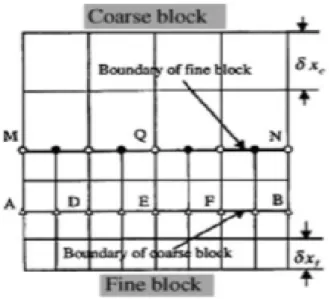
When the high resolution around the core jet is needed, the multi-block approach is used. An accurate interface treatment between neighboring blocks is derived by He et al [17], to satisfy the conservation of mass momentum and the continuity of stresses across the interface.

To illustrate the basic idea of grid refinement in our simulation, a horizontal plane three-block (coarse block, finer block and finest block) system as shown in Figure 2 is considered in the derivation for the interface information exchange. The ratio of the lattice space between the neighboring two blocks is

𝑛 = 𝛿𝑥_𝑐/𝛿𝑥_𝑓 (14)

13

For a given Re, in order to keep a consistent viscosity 𝜗 = (2𝜏 − 1)𝛿_𝑥/6, the relation between relaxation times 𝜏_𝑓 on the fine block and 𝜏_𝑐 on the coarse block must obey [18]

𝜏_𝑓= 1

2+ 𝑛(𝜏𝑐 − 1

2) (15) Since the velocity and density are continuous across the interface between two blocks, the equilibrium part across the interface follow:

𝑓_𝛼𝑒𝑞,𝑐(𝑥, 𝑡)=𝑓_𝛼𝑒𝑞,𝑓(𝑥, 𝑡) (16) In the LBER-LES with non-uniform mesh, we set 𝐶_𝑠2 = 0.16, and ∆_𝑥= 𝛿_𝑥 for each blocks, which means ∆_𝑥𝑐= 𝛿_𝑥𝑐 = 1 for coarse block, ∆_𝑥𝑓𝑖𝑛𝑒𝑟= 𝛿_𝑥𝑓𝑖𝑛𝑒𝑟 = 1/2 for finer block and ∆_𝑥𝑓𝑖𝑛𝑒𝑠𝑡= 𝛿_𝑥𝑓𝑖𝑛𝑒𝑠𝑡 = 1/4 for finest block.

At the interface, the spatial and temporal interpolation is needed [9]. The typical transverse surface structure is shown in Figure2. The time step size of a LBM

simulation is partially defined by the grid spacing, which is the spacing between two neighboring grid sites. For LBM simulation, the computations on the coarse grid and fine grid must be synchronized. The fine grid must perform the computations with several smaller steps to advance its simulation to the same time, as well as the simulation proceeds with one large time step on the coarse grid. At first, the global simulation on the coarse grid is running with a large time step 𝑡_𝑐, from the initial time 𝑇₁ to time 𝑇₃. Synchronously, the fine grid simulation is starting from time 𝑇₁ to

𝑇₂. When the fine grid simulation starts at time 𝑇₂, it runs with a smaller time step

𝑡𝑓(𝑡𝑐 = 2𝑡𝑓). The coarse grid computation does not provide the values of the particle distributions 𝑓_𝑖, on the interfaces at time 𝑇₂ due to its large time step size. Therefore, we perform a temporal interpolation to compute 𝑓_𝑖 at time 𝑇₂ from the global

14

computation results on the coarse grid at time 𝑇₁ and 𝑇₃, with the following scheme [12]: 𝑓_𝛼𝑐_{(𝑥, 𝑇} 2) = (1 − 𝑡𝑓 𝑡𝑐) 𝑓𝛼 𝑐_{(𝑥, 𝑇} 1) + 𝑡𝑓 𝑡𝑐𝑓𝛼 𝑐_{(𝑥, 𝑇} 3) (17) After the temporal interpolation, we have computed the particle distributions of grid sites on the coarse grid at time 𝑇₂. However, we still need more information for fine grid on the interface, which is the ‘ghost point’. Therefore, we execute a spatial interpolation to compute ghost point for fine grid on the interface with the second order 2D Lagrange interpolation [19].

2.3

Boundary condition

The bounce back boundary condition based on the idea of bounce back of the non-equilibrium part is implemented [20]. The primary boundary conditions are involved: no-slip boundary wall, periodic boundaries, and curve boundaries using

extrapolation approach [7].

Considering the uniform velocity flow field, the velocity boundary condition for the LBGK model is implemented. As D2Q9 LBGK example, the boundary is aligned with

𝑓₁, 𝑓₅, 𝑓₈ pointing into the domain. After streaming, 𝑓₀, 𝑓₂, 𝑓₃, 𝑓₄, 𝑓₆, 𝑓₇ are known. Suppose that 𝑢_𝑥= 𝑢_𝑖𝑛, 𝑢_𝑦 = 0 are specified on the wall and we want to use Eq. to determine 𝑓₁, 𝑓₅, 𝑓₈ and ρ, which can be put into the form

𝑓₁+ 𝑓₅ + 𝑓₈ = 𝜌 − (𝑓₀+ 𝑓₂+ 𝑓₄ + 𝑓₃+ 𝑓₆+ 𝑓₇) (18) 𝑓₁ + 𝑓₅+ 𝑓₈ = 𝜌𝑢_𝑥+ (𝑓₃+ 𝑓₆+ 𝑓₇) (19) 𝑓₅ − 𝑓₈ = 𝑓₄− 𝑓₂+ 𝑓₇ − 𝑓₆ (20) Equations (18-20) satisfy 𝜌 =(𝑓0+ 𝑓2+ 𝑓4+2(𝑓3+ 𝑓6+ 𝑓7)) 1−𝑢𝑥 (21)

15

We use the bounce back rule for the non-equilibrium part of the particle distribution normal to the inlet, to find 𝑓₁− 𝑓₁𝑒𝑞 = 𝑓₃ − 𝑓₃𝑒𝑞. With 𝑓₁ known, 𝑓₅, 𝑓₈ are obtained by the remaining two equations:

𝑓₁ = 𝑓₃+2 3 𝜌𝑢𝑥 (22) 𝑓₅ = 𝑓₇−(𝑓2−𝑓4) 2 + 𝜌𝑢𝑥 6 (23) 𝑓₈ = 𝑓₆+(𝑓2−𝑓4) 2 + 𝜌𝑢𝑥 6 (24)

In evolution, the distribution functions at the boundaries need to be specified according to the conditions for the macroscopic variables. Here we consider the velocity boundary conditions at the wall and use extrapolation method to apply the curve boundary condition at the circular boundary of the orifice. As it is shown in Figure 3, the link between the fluid node 𝑥_𝑓 and solid node 𝑥_𝑠 intersects the curve wall at the node 𝑥_𝑤. The fraction of the intersected link in the fluid region is defined as ∆=|𝑋_|𝑋𝑓−𝑋𝑤|

𝑠−𝑋𝑤|. After the collision step, the distribution functions 𝑓𝜕(𝑥𝑓, 𝑡) at the fluid node 𝑥𝑓 are known, however, we also need to know the distribution function

16

𝑓_𝜕(𝑥_𝑤, 𝑡) at the solid node 𝑥_𝑤 that moves from 𝑥_𝑤 to 𝑥_𝑓 in the streaming step. The so-called boundary condition here is to get 𝑓_𝜕(𝑥_𝑤, 𝑡). The basic idea of the

extrapolation method is to decompose 𝑓_𝜕(𝑥_𝑤, 𝑡) into the equilibrium and non-equilibrium functions. The non-equilibrium part could be determined by a fictitious equilibrium distribution, while the non-equilibrium part is approximated by that of neighboring fluid node along the link. Thus, the distribution function at the node 𝑥_𝑤

could be expressed as:

𝑓_𝛼(𝑥_𝑤, 𝑡) = 𝑓_𝛼𝑒𝑞(𝑥_𝑤, 𝑡) + 𝑓_𝛼𝑛𝑒𝑞(𝑥_𝑤, 𝑡) (25)

in the above equation, the equilibrium distribution could be approximated by a fictitious one: 𝑓_𝛼𝑒𝑞(𝑥𝑤, 𝑡) = 𝑤𝛼𝜌[1 + ( 3𝑒⃗⃗⃗⃗ ∙𝑢𝛼⃗⃗ 𝑤 𝑐2 + 9(𝑒⃗⃗⃗⃗ ∙𝑢𝛼⃗⃗ 𝑤)2 𝑐4 − 3 2 𝑢𝑤2 𝑐2 )] (26) with the velocity at the solid node could be chosen as followed relations:

𝑢𝑤 = { [𝑢_𝑏+ (∆ − 1)𝑢_𝑓]/∆, ∆≥ ∆_𝑐 𝑢_𝑏+ (∆ − 1)𝑢_𝑓+ 1−∆ 1+∆[2𝑢𝑏+(∆−1)𝑢𝑓𝑓] 1+∆ , ∆< ∆𝑐 (27)

while ∆𝑐 is the judgment parameter and in the current study ∆𝑐= 0.65 [7].

The non-equilibrium part could be approximated by the non-equilibrium part of the distribution function at the fluid nodes 𝑥_𝑓 and 𝑥_𝑓𝑓:

𝑓_𝛼𝑛𝑒𝑞(𝑥𝑤, 𝑡) =

{ 𝑓𝛼(𝑥𝑓, 𝑡) − 𝑓𝛼

𝑒𝑞

(𝑥𝑓, 𝑡), ∆≥ ∆𝑐

∆ (𝑓_𝛼(𝑥_𝑓, 𝑡) − 𝑓_𝛼𝑒𝑞(𝑥_𝑓, 𝑡)) + (1 − ∆) (𝑓_𝛼(𝑥_𝑓𝑓, 𝑡) − 𝑓_𝛼𝑒𝑞(𝑥_𝑓𝑓, 𝑡)), ∆< ∆_𝑐 (28)

2.4

pseudopotential Lattice Boltzmann Model

As a mesoscopic method with microscopic models, Lattice Boltzmann method (LBM) has an instinct kinetic nature and only involves simple algorithm with collision-streaming processes. The phase segregation and surface tension in multiphase flow

17

are due to the interparticle forces/microscopic interactions. The LBM is capable of incorporating these interactions without tracking/capturing the interface between immiscible phases/components. Hence, the LBM attracted attention in simulating multiphase flow. Shan and Chen [13] developed a potential multiphase LB model for multiphase and multi-component flows with introducing inter-particle interaction forces between fluid particles at neighboring lattice sites. The interaction potentials control the form of the equation of state (EOS) of the fluid. Phase separation occurs automatically when the interaction potentials are properly chosen. This interaction force includes two parts for the multi-component fluid. One is the interaction between molecules from the same component, 𝐹 𝑖,𝑖, and another is the interaction between molecules from different components, 𝐹 _𝑖,𝑗, which are calculated by the interaction potential. However, this pseudopotential model cannot satisfy the momentum conservation law at a local position and limited by the density ratio (maximum value is 10). In 2006, Yuan and Schaeffer [21] developed a relatively simple but effective method to incorporate various EOS into the pseudo potential model. The general idea is to associate the effective mass with different EOS i.e. vdW-EOS, C-S EOS and P-R EOS. The density ratio is only one defining characteristic of a MCMP flow system. A water-air system and an oil-air system perform very differently, although they have a similar density ratio. To capture these effects, the viscosity and the surface tension are two important factors [22]. For solid and wetting boundary, an additional force term should be introduced to the fluid-solid interaction, 𝐹 _𝑠,𝑖, which is dominated by above effective mass and an indicator

function that equals 1 for solid nodes and 0 for fluid nodes. Hence, the total force on each particle can be expressed as:

18

𝐹 _{𝑡𝑜𝑡𝑎𝑙,𝑖} = 𝐹 _𝜎,𝜎+ 𝐹 _𝜎,𝜎̅ + 𝐹 _𝑏,𝜎̅ + 𝐹 _𝑠,𝜎̅ (29)

These forces are represents respectively as shown below.

𝐹_𝜎,𝜎̅(𝑋) = −𝑐0𝜓𝜎(𝑋)𝑔𝜎𝜎̅𝛻𝜓𝜎̅(𝑋) (30)

𝐹_𝜎,𝜎(𝑋) = −𝑐0𝜓𝜎(𝑋)𝑔𝜎𝜎𝛻𝜓𝜎(𝑋) (31) where 𝑐0 is a constant that depends on the lattice structure. For the D2Q9 and D3Q19 lattices, 𝑐0 = 6.0, and for the D3Q15 lattice, 𝑐0 = 10.0 [22]. The coefficients for the strength of the interparticle force are gσσ̅ and gσσ, with negative value representing an attractive force between particles and positive value a repulsive force [23].

𝐹𝑏,𝜎(𝑋) = ∆𝜌𝑔 (32) where g is the acceleration of gravity,

𝐹_𝑠,𝜎(𝑋) = 𝑔𝑤𝜓(𝜌𝜎) ∑𝑁𝛼=1𝑤(|𝑒𝛼|2)𝜓(𝜌𝑠𝑜𝑙𝑖𝑑)𝑠(𝑥 + 𝑒𝛼)𝑒𝛼 (33) where g_w determines the strength of the interaction force between fluid and solid. In most studies employing the MCMP pseudopotential model, the interaction strength within each component, namely 𝑔𝜎𝜎 𝑎𝑛𝑑 𝑔𝜎̅𝜎̅ is set as zero, and only the interaction between different components 𝑔𝜎𝜎̅ contributes to the phase separation. Unfortunately, by using only one free parameter 𝑔𝜎𝜎̅ to control the two-fluid

system, the density ratio between the components is only unit and the maximum kinematic viscosity ratio achievable is less than 5 [15]. These forces can be

incorporated into the model by shifting the velocity in the equilibrium distribution. This means that the velocity 𝑢⃗ in the equilibrium equation is replaced by

𝑢⃗ _𝑖𝑒𝑞= 𝑢⃗ _𝑖 +𝜏𝑖𝐹 𝑡𝑜𝑡𝑎𝑙,𝑖

𝜌𝑖(𝑥 ) (34) Unlike in the original Shan and Chen model, the coefficient of interaction strength within a component (𝑔_𝑖,𝑖) here cannot control the overall interaction strength.

19

However, the coefficient of interaction strength between different components (𝑔_𝑖,𝑗) is very important for creating and extending the MCMP LBE model. The behavior of interactions between different components is mainly controlled by this force, so the interaction can be adjusted through changing the value of 𝑔_𝑖,𝑗. For MCMP model, this force usually plays a critical role in adjusting the system density ratio, which need to be investigated and explained in different cases.

The effective of mass can be defined as:

𝜓_𝜎(𝜌) = √2(𝑃𝜎−𝑐𝑠2)

𝑐0𝑔𝜎𝜎 (35) where p is the pressure. We implement Peng-Robinson (P-R) EOS into the effective mass, because P-R EOS provided a maximum increase in the density ratio while maintaining small spurious currents around the interface. The P-R EOS is expressed as: 𝑃 = 𝜌𝑅𝑇 1−𝑏𝜌− 𝑎𝛼(𝑇)𝜌2 1+2𝑏𝜌−𝑏2_𝜌2 (36) 𝛼(𝑇) = [1 + (0.37464 + 1.5422𝜔 − 0.26992𝜔2)(1 − √𝑇/𝑇𝑐)]2 (37) with a =0.4572𝑅2𝑇𝑐2 𝑃𝑐 , 𝑏 = 0.07788𝑇𝑐

𝑃𝑐 , where a is the attractive parameter, b is the repulsion parameter, R is the gas constant, ω is the acentric factor, and 𝑇_𝑐 and 𝑃_𝑐are the critical temperature and critical pressure, respectively. T is the temperature, since only isothermal systems are considered in our validation case, we set T as a constant, which equals 1.

2.5

openMPI parallel algorithm

The Message Passing Interface (MPI) is a message-passing library based on a distributed parallel programming model and achieves a process-level parallelism. It employs message passing for the necessary communication between the processes

20

running in parallel, to achieve parallelization of programs. Each of the processes involved has its own resources different from the others’. A process can send a message or data to another process and receive data from another process.

A process can send a message to all other processes in its” communication world” or in its group and gather data from them as well.

Figure 4 Schematic of domain decomposition along streamwise direction for openMPI parallel computing algorithm

We use C++ and openMPI library to implement parallel computing for the multi-phase LBM simulations. Figure 4 shows the concept of decomposition of the whole domain along the streamwise direction. With the definition of nodes number and rank size using,

21

MPI_Comm_size(MPI_COMM_WORLD, &numnodes); MPI_Comm_rank(MPI_COMM_WORLD, &mynode);

the whole domain is divided into couple segmentations and with several interfaces between two neighboring sub-domains created. The distribution functions on the interface of each node are packed as two-dimensional arrays and stored temporally. All the information transfer to the arrays of the interfaces belong to the neighboring nodes with MPI_SEND using same tag. Meanwhile, the arrays receive all the

information on the interfaces belong to the neighboring nodes with MPI_RECV using a different tag. After the transfer process, all the information is unpacked to the original four-dimensional distribution functions, then the LBM algorithm proceeds in every single node independently.

2.6

Summary

Our Lattice Boltzmann Method solver is build and developed using C++ based on classic BGK Lattice Boltzmann Method. In the solver, the multi-block is included for mesh refinement, and we use this approach to refine the mesh for simulations of the single-phase air jet flow issued from circular and lobed orifice. Results of these simulations are presented and discussed in Chapter 3. For high Reynolds number cases, the LES turbulence model is modified in our solver. In our single-phase and multi-phase jet breakup simulations, the LES model is applied. For the curve boundary, we implement the extrapolation approach to modify the circular jet orifice boundary condition. For water-silicon oil jet investigations, we build the multi-phase module using original Shan/Chen model. Using the benchmark of the static droplet without gravity force, Laplace analysis and three-dimensional droplet

22

including gravity force, we validated our multi-phase Lattice Boltzmann solver. We implemented the solver in liquid-liquid jet breakup simulations. Results of these simulations are presented and discussed in Chapter 4. Our single-phase simulations are parallelized using openMP and multi-phase simulations are parallelized using openMPI.

23

Chapter 3

Single-phase jet from circular and lobed orifice

3.1

Introduction

In the modern industry, air jets are widely used for diverse applications: including air supply for mechanical ventilation in buildings, heat exchange in industrial processes and aircraft propulsion, etc. Such flows are useful because of their intrinsic

properties of providing an efficient mixing by exchanging mass, momentum, heat. These flows are also encountered often since it is easily to generate them.

Figure 5 displays a schematic diagram of the expected general topology of a free circular jet [24]. With the orifice, the jet is blown with an nearly uniform flow velocity 𝑊₀ into the stationary ambient air. The vorticity layer rolls up, generating vortex and providing regularity of formation and evolution [25].

24

The shear layer structure influences the uniform core, that result in oscillation and reduction in the local mean velocity [26]. The generated vortices move downstream with the shear layer, due to the interaction between the jet core and ambient air [27]. The organized vortices break down, become unstable, decay to smaller structures, and eventually tune into fully developed turbulence. The decay can be triggered in two ways: 1) for low Reynolds number, the vortices are more likely to survive until the end of the potential core, where the inner border rotation region is met. In such case, the structure is symmetric and unstable [28]; 2) for higher

Reynolds number flow, the evolution of the vortices is more rapid than the previous case. The decay starts before the “self-closure”, therefore the large-scale structure cannot be observed around the later part of the core. The distance, from the exit section required for the roll-up, evolution, and decay of the vortices, is based on the Reynolds number and the thickness boundary layer [24].

For rectangular jets with an aspect ratio greater than 1, the azimuthal curvature variation of initial vertical structures produces non-uniform self-induction and three-dimensional structures. As a result, these flows spread out to the ambient with greater rate in the plane through the minor axis of their orifice exit than the one through major axis. In other words, as such flow proceeds downstream, the mean-flow cross-section tends to flip the minor and major axes at a certain distance from the orifice [29].

In noncircular jets studies, the axisymmetric lobed jet orifice geometry is usually included. It is applied as a baseline to quantify the relative mixing performance and to describe the behavior of the noncircular jet [30]. Two types of instabilities are

25

mainly presented in the simulations of asymmetric lobed jet: the primary Kelvin-Helmholtz instability (K-H) and secondary-type instability. The growing of the K-H structures results in the secondary-type instabilities of the braid between two successive rings [31]. Thus, it appears that the production of streamwise structures in the round jet is governed by the K-H rings. Unlike the circular jet, the streamwise structures in the non-circular jet are generated by the transverse shear that is

induced by the shape of the orifice, and may dominate the mixing phenomenon [32]. The main objective of this research is to investigate the mixing processes of the circular and lobed jets by studying the spread speed, the vortex generation, the core jet length, the main jet breakup, and the turbulence effects in the near fields of jet orifice. Next, we compare flow-fields of the circular and lobed jets in the near and transition fields. Boundary conditions, hydraulic diameters of the orifice and, Reynolds number are matched for comparisons of the circular and lobed. It aims at reporting the instantaneous/mean flow fields and the turbulence Reynolds stresses to quantify the differences/similarities between them.

In this chapter, we implement the single-phase Lattice Boltzmann Method along with LES turbulence model to handle high Reynold’s number jet flows. To reduce the computational requirement, the multi-block approach has been applied to refine the mesh around the core jet and jet orifice.

Single-phase jet flow simulations are conducted using openMP (for parallel

computing) on 16-core workstation. The total resolution with refined mesh is about 30 million and the total run time for each case is around 140 hours.

26

Source codes and post-processing codes are developed in C++ and run on Linux systems. Flow images are generated by TECPLOT.

Figure 6 Schematic representation of jet nozzle exit for circular and 6-lobde case; (a) Diameter of circular orifice exits; (b) equivalent diameter of 6-lobed nozzle exit

Figure 6 shows the shape and dimensions of the two orifice plates used in the present study. For the circular jet orifice, the orifice cross-section AR, is 1, and the hydraulic diameter is 40mm. The computational domain for the circular jets matches the experimental setup of Todde. V. et, al [24]. For the 6-lobed jet, the orifice cross-section AR, is 1.5. The hydraulic diameter is 𝐷_𝑒 = 12𝑚𝑚, which is similar to the experimental setup of by Mi. et, al [33]. Figure 7 illustrates the schematic diagram of the computational domain and boundary conditions imposed for the single-phase circular and 6-lobed jet flow simulations, and the details are discussed in the following sections.

Present orifice shapes and Dimensions (in millimeters). a. Circle: 𝐷_𝑒 = 𝐷 = 40𝑚𝑚,

𝐷𝑒

𝐷 = 1 and AR=1

b. 6-lobed rectangular orifice:

𝐷_𝑒 = 12𝑚𝑚 and AR=1.5 40 3 3 3 3 10 3 (a) _(b)

27

Figure 7 boundary conditions for single-phase circular and 6-lobed jet simulation

3.2

Single-phase jet from circular orifice

3.2.1

Simulation Setup

Reynolds number for different jet flow cases are listed in Table 1. The dimensions of the flow domain are 0.2m(L)*0.2m(W)*0.8m(H). The jet orifice is located at the center of the bottom plane, and the orifice has the hydraulic diameter 𝐷_𝑒 = 40 mm

related to the exit area S, with definition of 𝐷_𝑒 = √4𝑆/𝜋. The Reynolds number 𝑅𝑒_𝐷

is based on the hydraulic diameter and the uniform inlet velocity varying from 0.4 m/s to 26.7 m/s.

Table 1 Uniform exit velocity and actual exit Reynolds Number (built with the equiseta diameter and the exit velocity)

Test Case Uniform exit velocity (m/s) Exit Reynolds Number, 𝐑𝐞𝐃

1 2 3 4 5 0.4 0.62 1.0 1.5 2.5 1050 1620 2700 4050 6750 inlet outlet Peri o d ic b o u n d ar y Peri o d ic b o u n d ar y

Present domain and boundary setting of the single-phase circular and 6-lobed jet flow. The jet orifice locates on the no-slip bottom. The top is the fully developed outlet with zero gradient of velocity. The periodic boundary is applied for the sides.

28

We impose a non-dimensional uniform velocity and density (pressure) profile for the jet at the exit of the orifice: w₀ = 0.1 and 𝜌₀ = 1.0 (𝑃 = 𝑐 ∗ 𝜌₀). The desired

Reynolds number is selected, then the molecular viscosity 𝜗₀ is achieved with 𝑤₀ = 0.1 and 𝐷_𝑒 = 20 (in lattice units). Initially, the system is set at a quiescent state with

ρ = 𝜌₀ = 1.0 and u = v = w = 0 everywhere except at the jet orifice, where

𝑤 = 𝑤₀𝑧̂.

With the refined mesh and time step, the actual simulation time step is 0.002s, and the early stage results during 0-12s for all cases are shown in the following sections. Because for the downstream field fluids to reach fully developed state requires much longer domain length along streamwise direction than our setup, we present the near fields fluid flow visualizations and flow profiles in the results discussion section.

3.2.2

Mesh Refinement

In the application of LBM, one limitation to the numerical efficiency is that it is constrained by a special uniform lattice. The challenge of the uniform grid is how to offer high resolution near the jet orifice and core jet regions. It is desired to split the computational domain into grid blocks: within each block, uniform lattice spacing can be performed. For the grid block near jet orifice and core jet regions, the lattice separation is minimized, while the spacing could be large near the outer regions. The blocks are connected through the interfaces. An accurate interface treatment

between neighboring blocks can be derived to satisfy the conservation of mass and momentum and the continuity of stresses across the interface [12].

29

Figure 8 Structured mesh shown in XZ plane view

In the single-phase simulations, the domain size is two times finer in the fine block than that in the coarse one, which means the finer block contains 2 times finer mesh at the sub-block refined domain.

Between coarse, fine and finer blocks, two interfaces are introduced and need to be considered for the distribution functions transfer between each interface.

The information of the coarse block nodes is stored on the interface between two neighboring blocks temperately:

{ 𝑓𝑠𝑡𝑜𝑟𝑒 𝑐𝑜𝑎𝑟𝑠𝑒_{(𝑎, 𝑖, 𝑗, 𝑘) = 𝑓} 𝑖𝑛𝑡𝑒𝑟𝑓𝑎𝑐𝑒𝑐𝑜𝑎𝑟𝑠𝑒 (𝑎, 𝑖, 𝑗, 𝑘), 𝑓_{𝑠𝑡𝑜𝑟𝑒}𝑒𝑞,𝑐𝑜𝑎𝑟𝑠𝑒(𝑎, 𝑖, 𝑗, 𝑘) = 𝑓_{𝑖𝑛𝑡𝑒𝑟𝑓𝑎𝑐𝑒}𝑒𝑞,𝑐𝑜𝑎𝑟𝑠𝑒(𝑎, 𝑖, 𝑗, 𝑘) (38) { 𝑓𝑠𝑡𝑜𝑟𝑒 𝑓𝑖𝑛𝑒𝑟_{(𝑎, 𝑖, 𝑗, 𝑘) = 𝑓} 𝑖𝑛𝑡𝑒𝑟𝑓𝑎𝑐𝑒 𝑓𝑖𝑛𝑒𝑟 _{(𝑎, 𝑖, 𝑗, 𝑘),} 𝑓_{𝑠𝑡𝑜𝑟𝑒}𝑒𝑞,𝑓𝑖𝑛𝑒𝑟(𝑎, 𝑖, 𝑗, 𝑘) = 𝑓_{𝑖𝑛𝑡𝑒𝑟𝑓𝑎𝑐𝑒}𝑒𝑞,𝑓𝑖𝑛𝑒𝑟 (𝑎, 𝑖, 𝑗, 𝑘) (39)

It's then transferred from the temporarily storage to the fine blocks. However, some nodes on the interface of finer blocks do not exist on the interface of coarse blocks. Such nodes are so-called “Ghost nodes”. In order to get the information of the ghost

30

nodes for coarse blocks, both spatial and temporal interpolation is necessary to get the distribution function on the ghost nodes. For the spacing interpolation,

considering the viscosity terms, a 2nd _{order two-dimensional interpolation is applied:}

Forward one-dimensional interpolation for interface sides:

𝑓_{𝑠𝑡𝑜𝑟𝑒}(𝑎, 𝑖, 𝑗) =

(3𝑓𝑠𝑡𝑜𝑟𝑒(𝑎, 𝑖, 𝑗 − 1) + 6𝑓𝑠𝑡𝑜𝑟𝑒(𝑎, 𝑖, 𝑗 + 1) − 𝑓𝑠𝑡𝑜𝑟𝑒(𝑎, 𝑖, 𝑗 + 3)) (40)

Backward one-dimensional interpolation for interface sides:

𝑓𝑠𝑡𝑜𝑟𝑒(𝑎, 𝑖, 𝑗) =

(−𝑓_{𝑠𝑡𝑜𝑟𝑒}(𝑎, 𝑖, 𝑗 − 3) + 6 ∗ 𝑓_{𝑠𝑡𝑜𝑟𝑒}(𝑎, 𝑖, 𝑗 − 1) + 3 ∗ 𝑓_{𝑠𝑡𝑜𝑟𝑒}(𝑎, 𝑖, 𝑗 + 1)) (41)

Forward two-dimensional interpolation for the inner interface:

𝑓𝑠𝑡𝑜𝑟𝑒(𝑎, 𝑖, 𝑗) =

(9 ∗ 𝑓𝑠𝑡𝑜𝑟𝑒(𝑎, 𝑖 − 1, 𝑗 − 1) + 18 ∗ 𝑓𝑠𝑡𝑜𝑟𝑒(𝑎, 𝑖 + 1, 𝑗 − 1) − 3 ∗ 𝑓𝑠𝑡𝑜𝑟𝑒(𝑎, 𝑖 + 3, 𝑗 − 1) +

18 ∗ 𝑓𝑠𝑡𝑜𝑟𝑒(𝑎, 𝑖 − 1, 𝑗 + 1)+36 ∗ 𝑓𝑠𝑡𝑜𝑟𝑒(𝑎, 𝑖 + 1, 𝑗 + 1) − 6 ∗ 𝑓𝑠𝑡𝑜𝑟𝑒(𝑎, 𝑖 + 3, 𝑗 + 1) −

3 ∗ 𝑓𝑠𝑡𝑜𝑟𝑒(𝑎, 𝑖 − 1, 𝑗 + 3) − 6 ∗ 𝑓𝑠𝑡𝑜𝑟𝑒(𝑎, 𝑖 + 1, 𝑗 + 3) + 𝑓𝑠𝑡𝑜𝑟𝑒(𝑎, 𝑖 + 3, 𝑗 + 3))/64 (42) Backward two-dimensional interpolation for the inner interface:

𝑓𝑠𝑡𝑜𝑟𝑒(𝑎, 𝑖, 𝑗) =

(−3 ∗ 𝑓𝑠𝑡𝑜𝑟𝑒(𝑎, 𝑖 − 3, 𝑗 − 1) + 18 ∗ 𝑓𝑠𝑡𝑜𝑟𝑒(𝑎, 𝑖 − 1, 𝑗 − 1) + 9 ∗ 𝑓𝑠𝑡𝑜𝑟𝑒(𝑎, 𝑖 + 1, 𝑗 − 1) −

6 ∗ 𝑓𝑠𝑡𝑜𝑟𝑒(𝑎, 𝑖 − 3, 𝑗 + 1)+36 ∗ 𝑓𝑠𝑡𝑜𝑟𝑒(𝑎, 𝑖 − 1, 𝑗 + 1) + 18 ∗ 𝑓𝑠𝑡𝑜𝑟𝑒(𝑎, 𝑖 + 1, 𝑗 + 1) +

𝑓𝑠𝑡𝑜𝑟𝑒(𝑎, 𝑖 − 1, 𝑗 + 3) − 6 ∗ 𝑓𝑠𝑡𝑜𝑟𝑒(𝑎, 𝑖 − 1, 𝑗 + 3) − 3 ∗ 𝑓𝑠𝑡𝑜𝑟𝑒(𝑎, 𝑖 + 1, 𝑗 + 3))/64 (43)

For the temporal interpolation, a 1st _{order one-dimensional interpolation is adopted.}

After the interpolation for ghost nodes, all the information is transferred from the temporally storage including the ghost nodes to the finer block side interface by:

𝑓𝑓𝑖𝑛𝑒𝑟_{(𝑎, 𝑖, 𝑗, 𝑘) = 𝑓} 𝑠𝑡𝑜𝑟𝑒𝑐𝑜𝑎𝑟𝑠𝑒(𝑎, 𝑖, 𝑗, 𝑘) + ( 1 𝑟𝑒𝑓) ( 𝛺𝑐𝑜𝑎𝑟𝑠𝑒 𝛺𝑓𝑖𝑛𝑒𝑟) ( 1−𝛺𝑓𝑖𝑛𝑒𝑟 1−𝛺𝑐𝑜𝑎𝑟𝑠𝑒) (𝑓𝑠𝑡𝑜𝑟𝑒 𝑒𝑞,𝑐𝑜𝑎𝑟𝑠𝑒 (𝑎, 𝑖, 𝑗, 𝑘) − 𝑓𝑠𝑡𝑜𝑟𝑒𝑐𝑜𝑎𝑟𝑠𝑒(𝑎, 𝑖, 𝑗, 𝑘)) (44) Where ref is the refined times. In the solver, we use ref=2.

31

The calculation algorithm starts once the fine and finer blocks receive all the information from the interfaces. After the algorithm update the inside of the fine blocks, the information for the next time step is transferred back to the coarse blocks by: 𝑓𝑐𝑜𝑎𝑟𝑠𝑒_{(𝑎, 𝑖, 𝑗, 𝑘) = 𝑓} 𝑠𝑡𝑜𝑟𝑒 𝑓𝑖𝑛𝑒𝑟 (𝑎, 𝑖, 𝑗, 𝑘) +(𝑟𝑒𝑓) ∗ (𝛺𝑓𝑖𝑛𝑒𝑟 𝛺𝑐𝑜𝑎𝑟𝑠𝑒) ∗ ( 1−𝛺𝑐𝑜𝑎𝑟𝑠𝑒 1−𝛺𝑓𝑖𝑛𝑒𝑟) (𝑓𝑖𝑛𝑡𝑒𝑟𝑓𝑎𝑐𝑒 𝑒𝑞,𝑓𝑖𝑛𝑒𝑟 (𝑎, 𝑖, 𝑗, 𝑘) − 𝑓_{𝑖𝑛𝑡𝑒𝑟𝑓𝑎𝑐𝑒}𝑓𝑖𝑛𝑒𝑟 (𝑎, 𝑖, 𝑗, 𝑘)) (45) The flow chart of the computational procedure for the multi-block Lattice Boltzmann

Method is shown in Figure 9 [12].

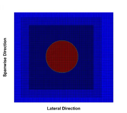
In our single-phase simulations, the whole domain is refined within three non-uniform meshes using multi-block approach as shown in Figure 8. The red region is the finest block around the jet orifice; the green region is the fine block relatively far from the jet orifice and around the core jet areas; the blue regions are the coarse blocks that away from the jet orifice and core jet areas. Because of the periodic boundary condition implanted for all four sides, the influence from coarse blocks near the side boundaries to the inside domain is acceptable.

32

Figure 9 Flow chat of the computational procedure using multi-block approach

1

Set initial values in all blocks

Algorithm in coarse blocks

Transfer information in coarse blocks to finer blocks

Spatial interpolation for ghost in fine blocks and store them in temporal storage

Algorithm in finer blocks

Same time level as coarse blocks

Transfer information in finer blocks to coarse blocks

End of total time steps

Output data files no

33

3.2.3

Boundary Conditions

For the bottom boundary, we implement uniform streamwise velocity for the jet orifice exit and the no-slip boundary condition for the bottom wall.

For the jet orifice:

𝑓₅ = 𝑓₆+ 𝑊₀∗ 𝜌₀/3 (46) 𝑓11= 𝑓14+ 𝑊0∗ 𝜌0 6 − 𝑓1−𝑓2+𝑓7−𝑓10+𝑓9−𝑓8 2 (47) 𝑓₁₂= 𝑓₁₃+ 𝑊₀∗𝜌0 6 + 𝑓1−𝑓2+𝑓7−𝑓10+𝑓9−𝑓8 2 (48) 𝑓₁₅= 𝑓₁₈+ 𝑊₀∗𝜌0 6 − 𝑓3−𝑓4+𝑓7−𝑓10+𝑓8−𝑓9 2 (49) 𝑓₁₆= 7 + 𝑊₀∗𝜌0 6 + 𝑓3−𝑓4+𝑓7−𝑓10+𝑓8−𝑓9 2 (50) For the no-slip bottom wall:

𝑓₅ = 𝑓₆+ 𝑊₀∗ 𝜌₀/3 (51) 𝑓₁₁ = 𝑓₁₄−𝑓1−𝑓2+𝑓7−𝑓10+𝑓9−𝑓8 2 (52) 𝑓₁₂ = 𝑓₁₃+𝑓1−𝑓2+𝑓7−𝑓10+𝑓9−𝑓8 2 (53) 𝑓₁₅ = 𝑓₁₈−𝑓3−𝑓4+𝑓7−𝑓10+𝑓8−𝑓9 2 (54) 𝑓₁₆ = 𝑓₁₇+𝑓3−𝑓4+𝑓7−𝑓10+𝑓8−𝑓9 2 (55) For the fully-developed top-outlet boundary [34]:

𝑓_𝑎(𝑛𝑧) = 𝑓𝑎(𝑛𝑧 − 1) (56) At this top boundary, we consider the zero Gradient of velocity,

𝑑𝑈

𝑑𝑛 = 0 (57) For side boundaries, periodic condition is imposed:

34

We follow the bounce back boundary condition by Zou/He [20] and modify the equilibrium part to reduce the information loss during the distribution function of collision on the boundary and bounce back processes. We focus on the core jet part and near jet orifice exit. The information loss is still acceptable around the no-slip wall and periodic boundaries.

Figure 10 schematic of refined mesh around circular jet nozzle exit

For the curved boundary condition, the extrapolation approach is applied to specify the distribution functions on the boundary that does not belong to any grid blocks. As in Figure 11, we consider the velocity boundary conditions at the wall node, which is the neighboring one and belongs to the no-slip bottom wall. Extrapolation method is applied to handle the boundary condition along the orifice circular side.

35

Figure 11 Lattice nodes of curved boundary

In these series of studies, the critical fraction of the intersected link in the fluid region: ∆𝑐 is set to 0.65. As discussed in the Chapter 2, we compare the defined fractions ∆, (where ∆=|𝑋𝑓−𝑋𝑤|

|𝑋𝑠−𝑋𝑤|) with ∆𝑐. If ∆> 0.65, the boundary node is closer to the outside the solid region, and we use the macroscopic information of the

neighboring nodes at solid region 𝑁_𝑤 and the fluid region 𝑁_𝑓 on the intersected link. If ∆< 0.65, the boundary node is closer to the inside fluid region, the macroscopic information of neighboring nodes at the solid region 𝑁_𝑤, the fluid region 𝑁_𝑓 and the successive fluid region nodes 𝑁𝑓𝑓 is then adopted.

3.2.4

Flow past cylinders

physical Boundary boundary node,b fluid node f wall node,w fluid node ff

36

Here we present the simulations of flow past two cylinders as a benchmark of our SRT Lattice Boltzmann Method solver and we compare the Karman vortex street and vortex-shedding phenomenon for validation.

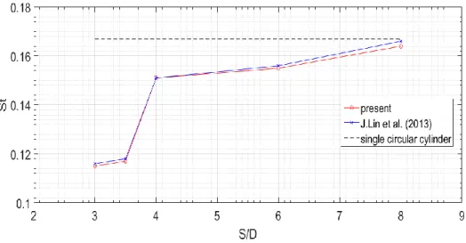
Flow past two tandem stationary cylinders in a uniform stream is a non-trivial nonlinear system, and previous studies demonstrates that the vortices separation between tow cylinders S/D has an important influence on the flow structure. In this section, such a flow configuration is investigated to validate our algorithm, the multi-grid non-uniform mesh model, and the curve boundary conditions with Re=100. The dimensionless computational domain is 25D (L)*10D (H) and the front cylinder center is located at 12.5D downstream of the inlet boundary and is on the centerline of the computational domain. The cylinder diameter is meshed with 20 lattices and the inlet free-stream velocity is V=0.1. The computed Strouhal number is presented in Figure 12. With the separation distance between two cylinders increases from 3D to 8D, Strouhal number increases. Similar trend has been reported by G.V.

Papaioannou, et al [35]. When S/D increases from 3 to 3.5, Strouhal number increases gradually, and it is significantly lower value than that from single circular cylinder case (𝑆𝑡_𝑠 = 0.167, as shown in the grey dash line). A sudden jump is

observed when S/D increases from 3.5 to 4. The mechanism of the jump is that once S/D increases beyond a critical value the vortex suppression region is translating to the co-shedding regime as the following contours shown.

37

Figure 12 Strouhal number versus scaled distance between two circular cylinders at Re=100

Figure 13 and Figure 14 show the results of flow patterns for the cases of S/D=3.5 and 4 obtained by LBM simulations, and the comparison to the work done by J. Lin et al [36]. The left panels indicate the instantaneous vorticity contours for S/D=3.5 cases, comparing to the results of reference J. Lin et al. [36]. With the free shear layers from the front cylinder reattach to the upstream side of the rear cylinder, the presence of the rear cylinder suppresses the vortex shedding from the front one and vortices are only shed behind the rear cylinder.

The right panels of each figure shows the cases of S/D=4.The vortices are shed from both cylinders, as shown in the contours, which leads to a sudden increase in the Strouhal number. As S/D is increasing further, the interaction from the two cylinders decreases and St approaches the value of the shedding frequency of vortices from the single circular cylinder. Our result has a good agreement with results reported by J. Lin et al [36].

38

(a) present LBM simulation S/D=3.5 (b) present LBM simulation S/D=4

Figure 13 Instantaneous vorticity contours for the flow past two stationary cylinders in tandem at Re=100 of LBM simulation results: Left is S/D=3.5 case; right is S/D=4.0 case

(a) J. Lin et al. [36] S/D=3.5 (b) J. Lin et al. [36] S/D=4

Figure 14 Instantaneous vorticity contours for the flow past two stationary cylinders in tandem at Re=100 of reference in Lin 2012: Left is S/D=3.5 case; right is S/D=4.0 case

3.2.5

Mesh Study

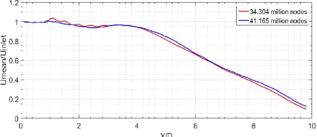
Although the LES method is a powerful tool in numerical simulation of turbulent flows and has less requirement in mesh size comparing to DNS, We should note that the LES method is still a turbulence model with modified small-scale structures of sub-grid flow field. Thus, the mesh convergence check is necessary. Figure 15 depicts the scaled centerline streamwise velocity obtained using two different mesh density levels at Re=72000. The resolution of coarse mesh is 34.304 million; the resolution of finer mesh is 41.165 million, which is 1.6 times finer than the ones in the original refined setup. No significant difference in the mean centerline streamwise velocity is observed; the decay location and spread out rate is similar between two different mesh sizes. Although notable difference is found at the area that is close to the jet orifice, it is still considered as a good match because this area is outside the main

39

interested region in our validations. Thus, the original mesh setup is sufficient to ensure spatial convergence in predicting the development of the flow fields.

Figure 15 The scaled mean centerline streamwise velocity vs the normalized length obtained by two different mesh density at Re=72000

3.2.6

Statistical Quantities: Mean Velocity

One of the most important phenomena in this study is the core jet length and velocity decay account of the jet breakup at the downstream region. The mean centerline streamwise velocity is the most important statistical representation of the core jet length and velocity decay phenomenon. Since the fluid in the tank is stationary initially, we should not consider the flow field until it is influenced by the impulsive start. For the following centerline streamwise mean velocity calculations, we collect the data with the time interval, from 2.0s to 10.0s. Velocity profiles are presented in non-dimensional units by scaling the distances to the jet orifice diameter and the velocities to the actual uniform inlet velocity. The normalized velocity is indicated as

𝑈∗ and is defined as

40

Figure 16 displays the mean centerline streamwise velocity distributions for all cases. The length D denotes the jet orifice diameter. This simulation domain has length of 20D in streamwise direction (z-axis). We present the profiles in 10D, because we set fully developed outflow boundary condition as the outlet. Such outlet simplifies the later part of the computational domain, in an unrealistic way, and hence the

effected region is less representative.

At lower Reynolds numbers, all the regions, up to approximately 6 diameters, shows an almost constant speed and no velocity decay. For all cases, in the region very close to the jet orifice (𝑍 < 0.5𝐷), small amplitude oscillations are noticed. This noise is more likely to be introduced by the boundary layer of the jet orifice.

Figure 16 Scaled mean centerline streamwise velocity of all different Reynolds number cases

The amplitude of the fluctuation depends on the Reynolds number. For the lowest Reynolds number case, Re=1050, the mean centerline streamwise velocity remains nearly constant until the start of the velocity decay at 6.5D, which is the location of the jet breakup. The jet decays linearly in the streamwise direction beyond 𝑍/𝐷 ≈ 6.5. For the intermediate Reynolds number flows (2700 ≤ 𝑅𝑒 ≤ 4050), the mean streamwise velocity decay happens closer to the jet orifice, which means the core jet