Diagnosing observation error correlations for Doppler radar radial winds in the Met Office UKV model using observation-minus-background and observation-minus-analysis statistics

Diagnosing observation error correlations 

for Doppler radar radial winds in the Met 

Office UKV model using observation­

minus­background and observation­

minus­analysis statistics 

Article 

Published Version 

Creative Commons: Attribution 4.0 (CC­BY) 

Open Access 

Waller, J. A., Simonin, D., Dance, S. L., Nichols, N. K. and 

Ballard, S. P. (2016) Diagnosing observation error correlations 

for Doppler radar radial winds in the Met Office UKV model 

using observation­minus­background and observation­minus­

analysis statistics. Monthly Weather Review, 144 (10). pp. 

3533­3551. ISSN 0027­0644 doi: https://doi.org/10.1175/MWR­

D­15­0340.1 Available at http://centaur.reading.ac.uk/65806/ 

It is advisable to refer to the publisher’s version if you intend to cite from the 

work. 

To link to this article DOI: http://dx.doi.org/10.1175/MWR­D­15­0340.1 

Publisher: American Meteorological Society 

All outputs in CentAUR are protected by Intellectual Property Rights law, 

including copyright law. Copyright and IPR is retained by the creators or other 

copyright holders. Terms and conditions for use of this material are defined in 

the 

End User Agreement  

. 

www.reading.ac.uk/centaur  

 

CentAUR 

Central Archive at the University of Reading 

Reading’s research outputs online

Diagnosing Observation Error Correlations for Doppler Radar Radial Winds

in the Met Office UKV Model Using Observation-Minus-Background and

Observation-Minus-Analysis Statistics

J. A. WALLER

School of Mathematical and Physical Sciences, University of Reading, Reading, United Kingdom

D. SIMONIN

MetOffice@Reading, University of Reading, Reading, United Kingdom

S. L. DANCE ANDN. K. NICHOLS

School of Mathematical and Physical Sciences, University of Reading, Reading, United Kingdom

S. P. BALLARD

MetOffice@Reading, University of Reading, Reading, United Kingdom

(Manuscript received 3 September 2015, in final form 7 June 2016) ABSTRACT

With the development of convection-permitting numerical weather prediction the efficient use of high-resolution observations in data assimilation is becoming increasingly important. The operational assimilation of these observations, such as Doppler radar radial winds (DRWs), is now common, although to avoid violating the assumption of uncorrelated observation errors the observation density is severely reduced. To improve the quantity of observations used and the impact that they have on the forecast requires the introduction of the full, potentially correlated, error statistics. In this work, observation error statistics are calculated for the DRWs that are assimilated into the Met Office high-resolution U.K. model (UKV) using a diagnostic that makes use of statistical averages of observation-minus-background and observation-minus-analysis residuals. This is the first in-depth study using the diagnostic to estimate both horizontal and along-beam observation error statistics. The new results obtained show that the DRW error standard deviations are similar to those used operationally and increase as the observation height increases. Surprisingly, the estimated observation error correlation length scales are longer than the operational thinning distance. They are dependent both on the height of the observation and on the distance of the observation away from the radar. Further tests show that the long correlations cannot be attributed to the background error covariance matrix used in the assimilation, although they are, in part, a result of using superobservations and a simplified observation operator. The inclusion of correlated error statistics in the assimilation allows less thinning of the data and hence better use of the high-resolution observations.

1. Introduction

With the recent development of convection-permitting numerical weather prediction (NWP), such as the Met Office U.K. variable resolution (UKV) model (Lean et al.

2008;Tang et al. 2013), the assimilation of observations that have high frequency both in space and time has be-come increasingly important (Park and Zupanski 2003;

Dance 2004;Sun et al. 2014;Ballard et al. 2016;Clark et al. 2015). The potential for assimilating one such set of observations, the Doppler radar radial winds (DRWs) (Lindskog et al. 2004;Sun 2005), has been explored by a number of operational centers (e.g.,Lindskog et al. 2001;

Salonen et al. 2007;Rihan et al. 2008;Salonen et al. 2009). The assimilation of the DRWs has been shown to provide a significant positive impact on the forecast (Xiao et al. 2005;Lindskog et al. 2004;Montmerle and Faccani

Corresponding author address: J. A. Waller, Department of Meteorology, University of Reading, Earley Gate, P.O. Box 243, Reading, RG6 6BB, United Kingdom.

E-mail: [email protected] Denotes Open Access content.

DOI: 10.1175/MWR-D-15-0340.1

2009;Simonin et al. 2014;Xue et al. 2013,2014) and as a result they are now included in operational assimilation (Xiao et al. 2008;Simonin et al. 2014).

Currently at the Met Office the error statistics associ-ated with DRWs are assumed to be uncorrelassoci-ated (Simonin et al. 2014). To reduce the large quantity of data and ensure the assumption of uncorrelated errors is rea-sonable the DRW observations are ‘‘superobbed’’ and thinned before assimilation (Simonin et al. 2014). These processes result in a large number of observations being discarded. To improve convection-permitting NWP it is necessary to make better use of high-frequency DRW observations. This requires less thinning of the observa-tional data, and hence the inclusion of correlated obser-vation error statistics in the assimilation system is required (Liu and Rabier 2003). Currently the full ob-servation error statistics associated with the DRWs are unknown. Therefore, the aim of this manuscript is both to estimate and to provide an understanding of the corre-lated observation errors associated with DRW.

In general, the errors associated with the observations can be attributed to four main sources: 1) instrument error, 2) error introduced in the observation operator, 3) errors of ‘‘representativity’’ (i.e., errors that arise where the observations can resolve spatial scales that the model cannot), and 4) preprocessing errors (i.e., errors introduced by preprocessing). For DRWs the instrument errors are independent and uncorrelated. Observation error correlations, which may be state dependent and dependent on the model resolution, are likely to arise from the other sources of error (Janjic´ and Cohn 2006;

Waller 2013;Waller et al. 2014a,b) (seesection 5bfor a more detailed description). The inclusion of correlated observation errors in the assimilation has been shown to lead to a more accurate analysis, the inclusion of more observation information content, and improvements in the forecast skill score (Stewart et al. 2013;Stewart 2010;

Healy and White 2005;Stewart et al. 2008;Weston et al. 2014). Significant benefit may even be provided by us-ing only a crude approximation to the observation error covariance matrix (Stewart et al. 2013; Healy and White 2005).

A number of methods exist for estimating the obser-vation error covariances (e.g., Hollingsworth and Lönnberg 1986;Dee and da Silva 1999).Xu et al. (2007)

presented an innovation method based on that of

Hollingsworth and Lönnberg (1986) for estimating DRW error and background wind error covariances.

Simonin et al. (2012)previously calculated observation error statistics for DRWs using the method ofXu et al. (2007). The work ofSimonin et al. (2012)suggests that the observation error standard deviation increases with the height of the observation and that the observations

errors have a correlation length scale of 1–3 km. How-ever, the Hollingsworth and Lönnberg (1986) method was initially designed to provide estimates of the back-ground error statistics under the assumption of un-correlated observation errors. The method can be used to estimate both correlated background and correlated observation errors; however, determining how to split the estimated quantity into observation and background errors is nontrivial (Bormann and Bauer 2010). Indeed the result is subjective. To overcome this difficulty most recent attempts to diagnose the observation error cor-relations have made use of the diagnostic proposed in

Desroziers et al. (2005). Initially designed as a consis-tency check, the diagnostic provides an estimate of the observation error covariance matrix using the statistical average of minus-background and observation-minus-analysis residuals. However, in theory it relies on the use of exact background and observation error statistics in the assimilation. Despite this limitation, the diagnostic has been used to estimate interchannel observation error sta-tistics (Stewart et al. 2009,2014;Bormann and Bauer 2010;

Bormann et al. 2010;Weston et al. 2014) even when the error statistics used in the assimilation are not exact. The method ofDesroziers et al. (2005)has also been used by

Wattrelot et al. (2012)to calculate observation error sta-tistics for the Doppler radial winds assimilated into the Météo-France system. Their results, published as a confer-ence paper, show a similar error standard deviation to those found inSimonin et al. (2012), but suggest that the obser-vation errors have a larger correlation length scale of ap-proximately 10 km (we cannot determine the length scale precisely because of the data thinning they have applied).

Here we present the first in-depth study using the di-agnostic ofDesroziers et al. (2005)to calculate obser-vation error statistics for the DRWs assimilated into the Met Office UKV model. Because of the limitations of the diagnostic we consider the sensitivity of the estimated observation error statistics to the choice of assimilated background error statistics. To aid our un-derstanding of the source of observation error we also consider the sensitivity of the estimated observation error statistics to the use of superobservations and the use of a more sophisticated observation operator. We find that, for summer season observations, the DRW error standard deviations are similar to those used op-erationally although, surprisingly, the observation error correlation length scales are longer than the operational thinning distance. Because of the uncertainty in the re-sults arising from the diagnostic the estimated correla-tion length scales should be interpreted as indicative, rather than necessarily quantitatively perfect. However, results from the diagnostics can still provide useful in-formation as further tests show that the long correlations

cannot be attributed to the background error covariance matrix used in the assimilation, although they may, in part, be a result of using superobservations and a sim-plified observation operator.

This paper is organized as follows. In section 2 we give a description of the diagnostic ofDesroziers et al. (2005). We describe the DRW observations and their model representations insection 3and insection 4we describe the experimental design. Insection 5we con-sider the estimated observation error statistics from four different cases. Finally we conclude insection 6. 2. The diagnostic of Desroziers et al. (2005)

Data assimilation techniques combine observations y2RNp with a model prediction of the state, the back-groundxb_2RNm

, often determined by a previous forecast. HereNp_andNm_{denote the dimensions of the observation}

and model state vectors, respectively. In the assimilation the observations and background are weighted by their respective errors, using the background and observation error covariance matricesB2RNm3NmandR2RNp3Np, to provide a best estimate of the state,xa_2RNm

, known as the analysis. To calculate the analysis the background must be projected into the observation space using the possibly nonlinear observation operator,H:RNp/RNm. After an assimilation step the analysis is evolved forward in time to provide a background for the next assimilation.

Desroziers et al. (2005) assume that the analysis is determined using

xa5xb1Ky2H(xb), (1) whereK5BHT(HBHT1R)21is the gain matrix andHis the linearized observation operator, linearized about the current state.

The diagnostic described in Desroziers et al. (2005)

estimates the observation error covariance matrix by using the minus-background and observation-minus-analysis residuals. The background residual, also known as the innovation,

do_b5y2H(xb) , (2) is the difference between the observation y and the mapping of the forecast vector,xb_{, into observation space}

by the observation operatorH. The analysis residual,

do_a5y2H(xa) (3)

’y2H(xb)2HKdo_b, (4) is similar to the background residuals, but with the forecast vector replaced by the analysis vectorxa_{. By}

taking the statistical expectation of the product of the analysis and background residuals results in

E[do_ado_bT]’R, (5) assuming that the forecast and observation errors are uncorrelated. Equation(5)is exact if the observation and background error statistics used in assimilation are exact. The theoretical work ofWaller et al. (2016)

provides insight into how results from the diagnostic can be interpreted when the incorrect background and observation error statistics are used in the as-similation. Because of the statistical nature of the diagnostic the resulting matrix will not be symmetric. Therefore, if the matrix is to be used it must be symmetrized.

3. Doppler Radar radial wind observations and their model representation

a. The Met Office UKV model and 3D variational assimilation scheme

The operational UKV model is a variable-resolution convection permitting model that covers the United Kingdom (Lean et al. 2008;Tang et al. 2013). The model has 70 vertical levels. The horizontal grid has a 1.5-km fixed resolution on the interior surrounded by a variable-resolution grid that increases smoothly in size to 4 km. The variable-resolution grid allows the downscaled boundary conditions, taken from the global model, to spin up before reaching the fixed interior grid. The initial conditions are provided from a 3D variational assimilation scheme that uses an incremental approach (Courtier et al. 1994) and is a limited-area version of the Met Office variational data assimilation scheme (Lorenc et al. 2000;Rawlins et al. 2007). The assimilation uses an adaptive mesh that allows the accurate representation of boundary layer structures (Piccolo and Cullen 2011,2012). The background error covariance statistics used in this study are described in

section 4.

b. Doppler radar radial wind data

Doppler radar is an active remote sensing instrument that provides observations of radial wind by measuring the phase shift between a transmitted electromagnetic wave pulse and its backscatter echo. The radial velocity of a scattering target is then estimated from the Doppler shift (Doviak and Zrnic´ 1993). While it is possible to derive clear air radar returns (e.g., Rennie et al. 2010,

2011), in this work we consider only observations where the scattering targets are assumed to be raindrops. The DRW data used at the Met Office are acquired using 18

C-band weather radars. Each radar completes a series of scans out to a range of 100 km every 5 min at different elevation angles (typically 18, 28, 48, 68, and 98) with a 18 3600 m resolution volume. Before being assimilated the data are processed and a quality control procedure is applied. This ensures that no observations that disagree with neighboring observations or have a large departure from the background are assimilated. The observa-tions errors are assumed Gaussian and uncorrelated in space or time with standard deviations that range from 1.8 m s21for observations close to the radar to 2.8 m s21 for observations farthest away from the radar. Further details of the operational assimilation of DRWs at the Met Office can be found inSimonin et al. (2014).

1) THE CURRENT OPERATIONAL OBSERVATION OPERATOR

To compare the background with the observations it is necessary to map the model state into observation space. The current operational observation operator, following

Lindskog et al. (2000), first interpolates the NWP model horizontal and vertical wind componentsu,y, andwto the observation location. The horizontal wind is then projected in the direction of the radar beam and pro-jected onto the slant of the radar beam using

yr5(usinf1ycosf) cos(u)1wsin(u) , (6)

wherefis the radar azimuth angle clockwise from due north anduis the beam center elevation angle. The el-evation angleu5«1aincludes a correction termathat must be added to the measurement elevation angle «. The correction term

a5tan21 rcos(«) rsin(«)1a_e1h_r , (7)

wherehris the height of the radar above sea level,ris the

range of the observation, andae is the effective Earth

radius (1.3 times the actual Earth radius) required to take account of Earth’s curvature and the radar beam refraction (Doviak and Zrnic´ 1993). The correction term is not exact. The value of ae is only valid in the

in-ternational standard atmosphere. This simple opera-tional observation operator does not account for the beam broadening or reflectivity weighting. Additionally, only the horizontal wind components are updated in the minimization, and the vertical component of wind is ignored, which for small elevation angles should be ac-ceptable. In addition no information about hydrometeor fall speed is available to the assimilation system.

This operational observation operator is used in the majority of results discussed in this article.

2) AN IMPROVED OBSERVATION OPERATOR

An improved observation operator has been trialled in the operational system; it accounts for some broad-ening of the beam (vertical only), as well as a reflectivity weighting. Both of these processes are often ignored in operational DRW assimilation (Ge et al. 2010). This improved observation operator is similar to the operator described byXu and Wei (2013), although it differs in some important details. The beam broadening model

Wbbtakes the form

W_bb(u_z)5exp 22 ln(2) u 2 z u2 3dB , (8)

withuz5u2ub, whereuis the beam center elevation as

in(6),ubis the elevation within the beam, andu3dBis the half power bandwidth (angular range of the antenna pattern in which at least half of the maximum power is still emitted; Toomay and Hannen 2004). For the re-flectivity weighting, a climatological profile with heighth

is used: W_ref(h)5Zh1c, (9) where Z5 26 dB:h,Brightband_L 22 dB:h.Brightband_U, (10)

cis a constant scaling factor, Brightband_L is the lower limit of the bright band, and Brightband_U is the upper limit of the bright band. The height of the bright band (a layer of melting ice resulting in intense reflectivity re-turn;Kitchen 1997) is derived from the forecast model temperature field, and has a thickness set to 250 m. The reflectivity profile increases by 10 dB from the bottom to the center of the bright band and then decreases linearly. The beam broadening and reflectivity weighting are combined to give a single weight,W5WrefWbband this weighting is included in the new observation operator:

y_r5

å

ML_u beam

W(usinf1ycosf) cos(u) . (11)

The summation in(11) is made over the model levels (ML_ubeam) present within the beam thickness. In this formulation,

å

Wis equal to one over ML_ubeam. The im-plementation of this new observation operator has been shown to reduce the error in the background residuals. This new observation operator may be further improved (Fabry 2010), although the operational use of a more complex observation operator may not be feasible. While these simplifications and omissions in the

observation operator exist, they will introduce addi-tional error when the model background is projected into observation space. These errors may well be cor-related and should ideally be accounted for in the ob-servation error covariance matrix.

3) SUPEROBSERVATION CREATION

To reduce the density of the observations, multiple observations are made into a single superobservation. Only observations that have passed the quality control procedure described inSimonin et al. (2014)are com-bined to make the superobservations. There are a num-ber of methods for calculating the superobservations. The Doppler radar superobservations used at the Met Office are calculated using innovations following the method of

Salonen et al. (2008). The radar scan is divided into 38by 3 km cells and one observation is created per cell using the following procedure:

1) Project background winds into observation space using(6).

2) Calculate the background residual at each observa-tion locaobserva-tion.

3) Average all background residuals that fall within a superobservation cell.

4) Add the average residual to the simulated back-ground radial wind at the center of the superobser-vation cell to give a value for the superobsersuperobser-vation. The calculated superobservations are subject to a second quality-control procedure (Simonin et al. 2014). They are then further thinned to 6 km, where it is assumed that the observations will have uncorrelated error, using Poisson disk sampling (Bondarenko et al. 2007).

4) SUPEROBSERVATION ERROR

The calculated superobservations have an associated superobservation error«so_{. The literature shows that the} superobbing procedure reduces the uncorrelated por-tion of the error; however, the correlated error is not reduced (Berger and Forsythe 2004). Berger and Forsythe (2004)showed that the covariance of the su-perobservation error will be equivalent to the averaged observation error covariance matrix for the raw obser-vations (i.e., creating the superobserobser-vations using the background does not introduce any background error into«so_{) if the following conditions are met:}

1) The observation and background errors are independent.

2) The background state errors are fully correlated within the superobservation cell.

3) The background state errors in a superobservation cell all have the same magnitude.

4) The background residuals are equally weighted within a superobservation cell.

However, for DRWs it is not clear that all the assump-tions will hold. In particular, assumpassump-tions 1 and 2 are valid at close range to the radar where the super-observation cells are small. However, at far range the superobservation cells are large and the assumptions are likely to be invalid. Therefore, it is possible that at large ranges there is a small influence of the background er-rors on the error associated with the superobservation.

5) ERROR SOURCES FORDOPPLER RADAR RADIAL WINDS

In the introduction the four main sources of obser-vation error are introduced. The obserobser-vation error will not only be a function of the observation type, but also of the observation preprocessing, observation operator and model resolution. Here we list some of the obser-vation error sources specific to DRWs:

d Errors introduced by clutter removal.

d Error introduced when creating the superobservations. d Misrepresentation of radar beam bending.

d Misrepresentation of beam broadening.

d Approximation of volume measurement as point measurement.

d Discrete approximation of continuous mapping from model to observation space.

d Errors of representativity. d Instrument error.

There may be additional unknown sources of error. It has been shown that some of these errors, such as the instrument error or those errors caused by the mis-representation of radar beam bending, are small (Xu and Wei 2013). However, there are other errors, such as the error introduced when creating the super-observations, misrepresentation of beam broadening, and the approximation of volume measurement as a point measurement, that we hypothesize will have a more significant contribution to the observation error statistics. Indeed,Fabry and Kilambi (2011)suggest that if the antenna beamwidth and reflectivity weighting are ignored in the observation operator, then the observa-tion errors will have long correlaobserva-tion length scales greater than 10 km.

4. Experimental design

To calculate estimates of the observation error co-variances we require background and analysis residuals. We use archived observations and background data pro-duced by the operational Met Office system from June,

July and August 2013. To generate the analyses we run four different assimilation configurations, detailed be-low. Using these backgrounds, analyses, and observa-tions we are able to determine the backgrounddoband

analysisdo_a residuals. Observations in this study come from 9 of the 18 radars in the network. Although ob-servation errors are likely to be state dependent (Waller et al. 2014b), we have used 3 months’ worth of data to ensure that we have enough data for the sta-tistical sampling error to be small. We have restricted ourselves to the summer season as we expect mainly convective rainfall (Hand et al. 2004;Hawcroft et al. 2012), which is likely to result in state-dependent ob-servation errors that are all similar.

Case 1 uses residuals produced by running the UKV under the January 2014 operational configuration. This uses superobservations (calculated as described in sec-tion 3b) thinned to 6 km and the observation operator given in(6). The background error covariance (‘‘New’’) has been derived using the Covariances and VAR Transforms (CVT) software, which is the new Met Of-fice covariance calibration and diagnostic tool that an-alyses training data representing forecast errors [either using the so-called National Meteorological Center (NMC) lagged forecast technique or ensemble pertur-bations]. Here an NMC method has been applied to (T16 h)2(T13 h) forecast differences to diagnose a variance and correlation length scale for each vertical mode.

Case 2 considers the effect of using the old (used prior to January 2013) operational UKV background error covariance matrix (‘‘Old’’). These statistics were gen-erated from (T124 h)2(T112 h) forecast differences; contrary to the CVT approach, the correlation functions used specific fixed length scales (Ballard et al. 2016). This background error covariance matrix has larger variances than the matrix used in case 1 and the corre-lation length scales are slightly longer. A comparison between cases 1 and 2 shows the impact of the assimi-lated background error covariance matrix on the esti-mated observation error statistics.

Case 3 uses the same background error covariance as case 1, but used raw observations (thinned to 6 km) rather than using the superobservations. A compari-son between cases 1 and 3 shows the impact of the superobservations on the estimated observation error statistics.

Case 4 uses the same design as case 3, the assimilation of raw observations, but the operational observation operator is replaced with the observation operator de-scribed in (11). A comparison between cases 3 and 4 shows the impact of the observation operator on the estimated observation error statistics.

We summarize the different cases inTable 1. For each case the available data for each radar scan are stored in 3D arrays of sizeNs_3Nr_3Na_{, whereN}s_is

the number of scans containing data, Nr_{516 is the}

number of ranges, andNa_{5120 is the number of}

azi-muths. Figure 1 shows a radar scan with the typical superobservation cells. The data are also separated by elevation, with data available at elevation angles 18, 28, 48, and 68. (We do not estimate the observation error statistics for the 98 beam due the lack of available data.) The position of these observations at these el-evations is shown in Fig. 2 (we note that the color scheme for each given elevation is used throughout the figures in this manuscript). It is important to note that these observations are only available in areas where there is precipitation and it is possible that only part of the scan contains observations. Furthermore, the use of the superobservations, thinning, and quality control results in a limited amount of data in each scan. The amount of data available differs for each elevation, with data for the lower elevations available out to far range (a result of the quality control procedures) and for higher elevations available only for near range. This lack of data means that standard deviations and correlations are not available for every range at each elevation. Results are only plotted for standard de-viations if 1500 or more samples were available and for correlations if the number of samples was greater than 500. The minimum number of samples is chosen to ensure that sampling error does not contaminate our estimates of the error statistics. Observations may be correlated along the beam, horizontally or vertically. Here we consider both horizontal correlations and those along the beam.

Horizontal correlations consider how observations at a given height are correlated. The blue cells inFig. 1

show a set of observations that would be compared for a given height. For each radar scan, data are sorted into 200-m height bins. Here the height takes into account the height of the radar above sea level. All observations that fall into a particular height bin are considered. The data are binned by separation distance for each pair of observations and from this the correlations are calculated.

TABLE1. Summary of experimental design for different cases. Case B Superobservations

Observation operator 1 New Yes Old 2 Old Yes Old 3 New No Old 4 New No New

When calculating along-beam correlations we con-sider how observations in the same beam are correlated to each other, where correlations are expressed for the separation distance along the beam. The red cells in

Fig. 1show one set of observations that would be con-sidered in this case. Here the samples used for calcu-lating(5)are taken to be the individual scans along the azimuth. Samples are taken on all dates, from all radars, and from each azimuth. When calculating results along the beam we do not expect to obtain symmetric corre-lation functions. When considering the along-beam correlations at any given range the positive separation distance will result in a different correlation to the

negative separation distance. For example, say we are considering the correlations for the observation lo-cated at 30-km range; the correlation with the 18-km observation (212-km separation) will have a smaller measurement volume whereas the observation at 42 km (112-km separation) will have a larger mea-surement volume. This is an important factor to con-sider when analyzing the along-beam correlation results. When plotting the along-beam correlation functions, it can appear as though the plot is in-complete for data at low elevation, far range, and high height (e.g., Figs. 10 and 11). This is a result of the range limit of the radar. For example, as depicted in

FIG. 1. A typical radar scan where each box is the location of a superobservation. The blue cells show a group of observations, all at the same height, that would be compared to calculate horizontal correlations. The red cells show observations that would be compared to calculate the along-beam correlations.

Fig. 2, at an elevation of 18and height of 2.5 km, the range of the observation is 94 km. There are no ob-servations available beyond a range of 100 km from the radar, so therefore we are unable to calculate the correlation beyond a separation distance of 16 km (i.e., 6 km farther from the radar).

For both horizontal and along-beam correlations it is possible to calculate an average correlation function using all available data that is homogeneous for all elevations, heights, and ranges. These average correlation functions provide an overall impression of how the calculated co-variance differs between cases. The average along-beam correlation functions are also comparable to those calcu-lated inWattrelot et al. (2012). The disadvantage of this method is that different elevations represent different heights in the atmosphere, and also have interaction with different model levels. Therefore it is difficult to dis-tinguish how the error correlations arise, whether they are a result of errors in the observation operator or arise from the misrepresentation of scales. In an at-tempt to understand exactly what is contributing to the error we also calculate the correlations for different elevations separately as this allows us to better un-derstand the origin and behavior of the errors.

5. Results

a. Case 1—Results from the operational system

We begin by calculating the observation error co-variances for case 1. Here data were acquired using the January 2014 operational system. This uses super-observations (calculated as described in section 3) thinned to 6 km, the observation operator given in(6), and the new background error covariance statistics.

1) HORIZONTAL CORRELATIONS

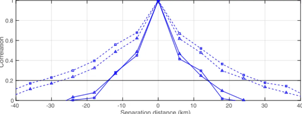
We first calculate the average horizontal correlation function using all data from all elevations. We show the standard deviation for this case inTable 2and the corre-lation in Fig. 3. (Note that the table and figure contain results for all cases; in this section we discuss the results for case 1 only). The standard deviation falls within the range of operational DRW standard deviations. We see that the estimated correlation length scale [defined to be the dis-tance at which correlation becomes insignificant (,0.2);

Liu and Rabier 2002] is approximately 24 km. This is much larger than the distance of 1–3 km calculated inSimonin et al. (2012)using the method ofXu et al. (2007)and the operational thinning distance of 6 km. This indicates that the assumption of uncorrelated errors is incorrect.

We now consider the horizontal correlations for dif-ferent heights and each elevation separately. InFig. 4we plot the standard deviation with height for each eleva-tion. We see that the standard deviations increase with height, with the exception of the lowest levels, and are similar for each elevation. For each elevation, the vol-ume of atmosphere sampled by the observation in-creases with height. (Note that at any given height the volume sampled by the 68beam will be smaller than the 18beam). Observations that sample larger volumes are

TABLE 2. Horizontal and along-beam standard deviations calculated for cases 1–4 using all available data up to a height of 5 km. Case Horizontal standard deviation (m s21) Along-beam standard deviation (m s21) 1 1.97 1.95 2 1.57 1.59 3 1.96 1.99 4 1.82 1.89

FIG. 3. All elevation horizontal observation error correlations for case 1 (control; squares), case 2 (alternate background error statistics; diamonds), case 3 (thinned raw data; triangles), and case 4 (new observation operator; circles). Error correlations are deemed to be insignificant below the horizontal line at 0.2.

expected to have a larger instrument error as the Doppler shift is calculated from multiple scattering targets in the measurement volume. In addition, these observations will be subject to more error from the observation oper-ator as only information from the model level nearest to the center of the sample volume is utilized, even when the sample volume spans several model layers. The increased errors at the lowest height may be a result of larger rep-resentativity errors as the observations at the lower heights sample smaller volumes than the model resolu-tion. Our results support previous work inSimonin et al. (2014)and we find that the standard deviations are sim-ilar to those used operationally.

Next we consider how the horizontal correlation length scale changes for a given elevation at different heights. We plot the calculated correlation functions for a range of

heights inFig. 5. We see that the correlation length scale increases with height and ranges between 17 and 32 km. For all heights the correlation length scale is longer than the operational thinning distance. An increase in height corresponds to an increase in both the distance of obser-vation away from the radar and the volume of the mea-surement box and therefore the change in correlation length scale could be attributed to either of these variables. In an attempt to determine the cause of the change in length scale we consider the horizontal correlations at the 2.5-km height for the different elevations. At any given height the measurement volume of the observation is larger for lower elevations.Figure 6shows that the cor-relation length scales are larger for the lower elevations. This suggests that it is the change in measurement volume that affects the correlation length scale. As in this case the

FIG. 4. Horizontal observation error standard deviation for elevations 18(black), 28(blue), 48(red), and 68(cyan) for case 1 (control; squares), case 2 (alternate background error statistics; diamonds), case 3 (thinned raw data; triangles) and case 4 (new observation operator; circles).

FIG. 5. Horizontal observation correlations for elevation 28at heights 1.1 km (dotted), 2.7 km (dashed), 3.5 km (solid), and 4.3 km (dot–dashed) for case 1 (control). Error correlations are deemed to be insignificant below the horizontal line at 0.2.

observation operator does not account for the observa-tion volume, it is likely that the correlated error is, in part, caused by the error in the observation operator.

It is also possible to compare observations at the same range, observations will have the same mea-surement volume but will be at different heights in the atmosphere. In this case we find that for each eleva-tion the correlaeleva-tion length scale is similar (e.g., at a range of 40 km each elevation has a correlation length scale of ;23 km; not shown). This suggests that the measurement volume of the observation has the largest impact on the horizontal correlation length scale, with correlation length scale increasing with measurement volume.

2) ALONG-BEAM CORRELATIONS

Next we calculate the along-beam observation errors using the data from case 1. We begin by calculating the

average observation error covariance and comparing these results with those from Météo-France (Wattrelot et al. 2012). We do not expect estimated statistics to be equal to those found by Météo-France as there are differences in the operational setup (e.g., observation and background error covariance statistics, observa-tion processing, observaobserva-tion operators, and thinning distances) and the region and time scale covered by the data.

Our estimated standard deviation (Table 2) is larger than the standard deviation found by Météo-France, which is 1.51 m s21. This is likely to be the result of the different operational setup and observation process-ing. We plot our estimated correlation function along with the correlation found by Météo-France inFig. 7. We see that the correlation length scales are approx-imately 5 km longer than those found by Mété o-France. Given the different operational setup used by

FIG. 6. Horizontal correlations at height 2.5 km for elevations 18(black), 28(blue), 48(red), and 68(cyan) for case 1 (control). Error correlations are deemed to be insignificant below the horizontal line at 0.2.

FIG. 7. All elevation along-beam observation error correlation for cases 1 (control; squares), 2 (alternate background error statistics; diamonds), 3 (thinned raw data; triangles), and 4 (new observation operator; circles) and those found previously by Météo-France (crosses). Error correlations are deemed to be insignificant below the horizontal line at 0.2.

Météo-France, the similarities between the results are reassuring and suggest that we are obtaining a reasonable estimate of the observation error correlations.

Next we calculate the error statistics along the beam for each elevation. InFig. 8(square symbols) we plot the change in standard deviation with height for beam ele-vations of 18, 28, 48, and 68. (For the horizontal correla-tions the height of the radar above sea level was accounted for; here height is calculated assuming that the radar is at sea level). For all elevations the obser-vation error standard deviation generally increases with height, with the exception of the lowest levels. This is similar to the behavior of the standard deviations for the horizontal case. Unlike the horizontal case the standard deviations for each elevation are not so similar. For any

given height the standard deviations are larger for the lower elevations. At any given height the lower eleva-tions will be sampling larger volumes of the atmosphere. Observations sampling large volumes are subject to both larger instrument error and more error in the observa-tion operator.

We now consider how the correlation length scale changes for a given elevation at different heights. The estimated observation error correlations for a range of heights are plotted inFig. 9. The along-beam correlation length scales are shorter than the horizontal correla-tions, although the correlation length scale still increases with height for any given elevation. This highlights the relationship between the increase in correlation length scale with the increasing height, range, and volume measurement of the observation.

FIG. 8. Along-beam observation error standard deviation for elevations 1₈(black), 2₈(blue), 4₈(red), and 6₈(cyan) for case 1 (control; squares), case 2 (alternate background error statistics; diamonds), case 3 (thinned raw data; triangles), and case 4 (new observation operator; circles).

FIG. 9. Along-beam observation correlations for elevation 28at heights 1.1 km (dotted), 3.0 km (dashed), and 3.5 km (solid) for case 1 (control).

In Fig. 10we consider how the correlation function differs with measurement volume. We plot the along-beam correlation function for each elevation at a height of 2.5 km. Here the height for each observation is the same, but the measurements are taken at different ranges with the lowest elevation at the farthest range.

Figure 10 shows that the correlation length scale in-creases with range. Again this is likely to be a result of the larger measurement volumes at far range.

InFig. 11we plot the correlation function for each elevation at a range of 40 km. Here the volume of measurement for each observation is the same, but measurements from lower elevations are at lower heights. We see that the correlation length scale differs with ele-vation and decreases with height. We hypothesize that the change in correlation is a result of the different levels of the atmosphere sampled by different beam elevations.

For the low elevation angles the beam gradient is shallow, hence different gates measure similar heights in the atmosphere; this results in larger error correla-tions. Larger elevation angles have larger beam gra-dients, and different gates sample a wider range of heights in the atmosphere; this results in small obser-vation error correlations.

3) SUMMARY

For this case we have calculated observation error statistics using background residuals from June, July, and August 2013, the analysis residuals are produced by running the UKV model using the January 2014 oper-ational configuration. We find the following:

d DRW standard deviations increase with height (with the exception of the lowest heights). This is likely due

FIG. 10. Correlations along the beam at height 2.5 km for elevations and approximate ranges 18 ’94 km (black), 28 ’64 km (blue), 48 ’35 km (red), and 68 ’22 km (cyan) for superobbed data (squares/solid lines) and thinned raw data (triangles/dashed lines). Error correlations are deemed to be insignificant below the horizontal line at 0.2.

FIG. 11. Correlations along the beam at range 40 km for elevations and approximate heights 18 ’0:8 km (black), 28 ’1:5 km (blue), 48 ’3:0 km (red), and 68 ’4:3 km (cyan) for super-obbed data (solid lines) and thinned raw data (dashed lines). Error correlations are deemed to be insignificant below the horizontal line at 0.2.

to the increasing measurement volume with height. The larger errors at the lowest height are likely to be a result of representativity errors.

d The correlation length scale is larger than the thinning distance of 6 km chosen to ensure that the assumption of uncorrelated errors is valid.

d For both horizontal and along-beam correla-tions and for all elevacorrela-tions the observation error correlation length scale increases with height. We hypothesize that this is in part due to the larger errors in the observation operator and correlated superobservation errors at large range. This will be the subject of further investigation (seesections 5c

and5d).

b. Case 2—The effect of changing the assimilated background error statistics

The diagnostic of Desroziers et al. (2005) uses the assumption that the observation and background error covariance matrices used in the assimilation are exact. In the operational assimilation, case 1, the observation errors are assumed uncorrelated and the background error variance and correlation length scale are believed to be too large. (The Met Office has an ongoing project to develop an improved background error covariance matrix; this is expected to reduce error variances and correlation length scales compared to those used in case 1 of this study.) Results given inWaller et al. (2016)

relating to the diagnostic suggest that under these cir-cumstances the diagnostic will underestimate the ob-servation error correlation length scale. Therefore it is possible that the true observation error statistics have longer correlation lengths than those calculated for case 1.

To provide information on how results in case 1 may compare to the true observation error statistics, we consider the sensitivity of the estimated observation error statistics to using different background statistics. Here we use previous operational background error statistics that have larger variances and larger length scales than the background error statistics used in the previous experiments.

1) HORIZONTAL CORRELATIONS

The average standard deviation given in Table 2

shows that the use of background error statistics with larger variance and longer length scales results in a lower estimate of the observation error standard de-viation. The correlation function, plotted inFig. 3, shows clearly that using a different background error co-variance matrix has reduced the estimated observation error correlation length scale. These results agree with

the theoretical results in Waller et al. (2016) (larger overestimates of variance and correlation length scale in the assimilated background statistics result in more se-vere underestimates of observation error variance and correlation length scale) and suggest that the theoretical results developed under simplifying assumptions are still applicable in an operational setting. The theoretical work and results from cases 1 and 2 suggest that if the variances and length scales in the assumed covariance matrixBwere further reduced compared to case 1, the estimated observation error correlation length scales would be larger.

Figure 4shows that the change in standard deviation with height for each elevation is similar to case 1. However, the standard deviations for case 2 are smaller than those from case 1, a result of the larger background error variances used in the assimilation.

As with the average correlations, results relating to the correlations for each individual elevation and height have smaller correlation length scales than case 1 (not shown). However, we still find that the quali-tative behavior of the correlation length scales remains the same; that is, for any elevation the cor-relation length scale increases with height and for any given height the length scale decreases as elevation increases.

2) ALONG-BEAM CORRELATIONS

For the average along-beam correlation we find the standard deviation (Table 2) is reduced compared to case 1. The correlations plotted in Fig. 7 also have a shorter length scale (approximately 10 km) and are more comparable to those found by Météo-France.

When considering the standard deviations for each elevation we again see that they are reduced (see di-amonds inFig. 8), although the change in standard de-viation with height is qualitatively similar to case 1. We find that the shape of the correlation function is similar, but the length scales are shorter than those calculated in case 1 (not shown). The variation in the correlation length scale with elevation, height, and range is, how-ever, unaltered.

3) SUMMARY

For this case we have calculated observation error statistics using different background error statistics that have larger variances and correlation length scales. We find the following:

d Estimated observation error standard deviations (length scales) are smaller (shorter) when using the alternative background error statistics with larger standard deviations and longer correlation length

scales. This result follows the theoretical work of

Waller et al. (2016).

d Changes in observation error standard deviation and correlation length scale with height remain qualita-tively similar to case 1.

d Given that the background error standard deviations and correlation length scales in case 1 are believed to be too large and long, it is likely that the true observa-tion error statistics have larger standard deviaobserva-tions and longer length scales than those calculated in case 1.

c. Case 3—The effect of the superobservations

The creation of the superobservations, discussed in

section 3b, results in an observation error that is only independent of the background error if the errors in the background states used in the calculation of each su-perobservation are of the same magnitude and are fully correlated (Berger and Forsythe 2004). This assumption is true at close range to the radar, but it is possible that it is violated at far range resulting in increased observation error correlation length scales. To determine if the su-perobservations have this effect we consider the results from case 3, where the assimilation uses thinned raw data. We return to using the new background error statistics.

1) HORIZONTAL CORRELATIONS

Table 2shows that the average standard deviation for this case is very similar to that of case 1. However, the correlation length scale is slightly reduced compared to case 1 (Fig. 3). This suggests that the use of super-observations may introduce some observation error correlation but does not appear to be the main source of correlations.

Figure 4shows that the standard deviations for indi-vidual elevations are similar to those found in case 1. In general we find that the use of the thinned data results in slightly shorter observation error correlation length

scales for observations that are at lower elevations and far range. For example,Fig. 12shows, for the 28 eleva-tion, that the use of the superobservations has little impact on the correlation length scale at short range. However, at far range the correlation length scale for case 1 is approximately 5 km longer than that for case 3. This result supports our hypothesis that the use of su-perobservations increases the observation error corre-lation length scale at far range. This is a result of the invalid assumption that the errors in the background states used in the superobservation creation are of the same magnitude and fully correlated.

2) ALONG-BEAM CORRELATIONS

From Table 2we see that the average along-beam observation error standard deviation is similar to that found using the data from case 1.Figure 7shows that the correlation length scale is also slightly reduced.

Figure 8shows that the standard deviations for sepa-rate elevations are similar to case 1.Figures 10and11

show that using the raw observations results in a simi-larly shaped correlation function to case 1 but with a slightly reduced length scale. The exception is the highest elevation (closest range) where the length scales are slightly larger. These results suggest that using the superobservation has the opposite effect, namely the introduction of correlation at far range, but a reduction of correlation in the higher elevations.

3) SUMMARY

We have calculated observation error statistics using thinned raw observations. We make these findings: d Using thinned raw data has little impact on the

estimated observation error standard deviations; this is similar to case 1.

d In general, horizontal correlation length scales at far range are reduced. This implies that using

super-FIG. 12. Horizontal observation correlations for elevation 28at a range of 24 km (solid) and 90 km (dashed) for case 1 (control; squares) and case 3 (thinned raw data; triangles). Error correlations are deemed to be insignificant below the horizontal line at 0.2.

observations introduces correlated error at far range, possibly as a result of an invalid assumption in the superobservation creation.

d In general along-beam correlation length scales are reduced for the lower elevations; however, they are slightly increased for the 68beam.

d. Case 4—The effect of an improved observation operator

The previous cases have all used the simplified ob-servation operator described in(6). The omission of the more complex terms introduces both additional error variance and correlation (Fabry 2010). It may not be possible to use a full observation operator in opera-tional assimilation, although the use of the sophisti-cated observation operator in(11)may be considered. In this case we use this new observation operator to see if including beam broadening and reflectivity weighting in the observation operator has any effect on the observation error statistics. Here we use the thin-ned raw observations rather than the superobservations (the creation of the superobservation involves the obser-vation operator, and ideally we wish to isolate the impact of the observation operator in the assimilation), so the results here must be compared to case 3.

1) HORIZONTAL CORRELATIONS

For the average horizontal error statistics both the standard deviation and correlation length scale have decreased compared to case 3 (seeTable 2andFig. 3).

For the separate elevations, as with all previous cases, we find that the standard deviations increase with height (Fig. 4), although here the actual values for the lower elevations are reduced compared to the standard de-viations found in case 3. The reduction is not seen in the higher elevations as observations are at near range

where the effects of beam bending and broadening, ac-counted for in the new observation operator, are not so significant. In general, we find that the correlations for every elevation are decreased when using the improved observation operator. InFig. 13we show that using an improved observation operator reduces the correlation length scale slightly at near range, and at far range by approximately 40%.

When considering horizontal correlations we com-pare observations at the same range away from the radar that have the same measurement volume, and hence the new observation operator should have the same im-provement for each observation we compare. The re-duction in error standard deviation and correlation shows that the inclusion of the beam broadening and reflectivity weighting has improved the observation operator. It also suggests that the use of an even more sophisticated observation operator may further reduce the observation error correlation.

2) ALONG-BEAM CORRELATIONS

In this caseTable 2and Fig. 8show that the error standard deviation is reduced compared to case 3, suggesting that the more sophisticated observation operator is indeed an improved map from background to observation space. BothFig. 7and the correlations for separate elevations suggest that introducing the new observation operator slightly increases the corre-lation length scale. We hypothesize that this is a result of the inclusion of the beam broadening. When using the old observation operator observations at different ranges at any elevation were unlikely to consider data from the same model levels. With the introduction of the beam broadening different observations will now use information from the same model levels and this is

FIG. 13. Horizontal observation correlations for elevation 18at a range of 18 km (solid) and 74 km (dashed) for case 3 (thinned raw data; triangles) and case 4 (new observation operator; circles). Error correlations are deemed to be insignificant below the horizontal line at 0.2.

likely to be the cause of the increased correlation length scales.

3) SUMMARY

For this case we have calculated observation error statistics using thinned raw observations and an im-proved observation operator. We find the following: d Using the new observation operator reduces the error

standard deviations for the lower elevations. Less impact is seen in the higher elevations where the effects of beam bending and broadening (accounted for in the new observation operator) are not so significant. d For the horizontal correlations using the new

obser-vation operator reduces the estimated obserobser-vation correlation length scale. This suggests that error in the observation operator may be in part responsible for the large correlation length scales.

d Using the new observation operator increases the along-beam correlation. This is likely to be the result of close observation residuals sharing increased amounts of background data.

6. Conclusions

With the development of convection-permitting NWP the assimilation of high-resolution observations is be-coming increasingly important. Currently large quanti-ties of high-resolution data are discarded to ensure the assumption of uncorrelated observation errors is rea-sonable. The assimilation of high-resolution observa-tions will require less thinning of the observational data and, hence, the inclusion of correlated observation error statistics in the assimilation system. Observation errors can be attributed to a number of different sources, some of which may be state dependent and dependent on the model resolution. Calculation of observation error sta-tistics is difficult as they cannot be measured directly. Recently the diagnostic of Desroziers et al. (2005)has been used to estimate interchannel observation error correlations for a number of different observation types. When inexact background and observation errors are used in the assimilation cost function, theory (Waller et al. 2016) shows that the results arising from the di-agnostic are uncertain and should be interpreted as in-dicative, rather than necessarily quantitatively perfect. However, results from the diagnostics can still provide useful information on the sources of error correlation and how it may be reduced. Furthermore, idealized studies using correlated observation error matrices in-dicate that much of the benefit in assimilation accuracy can be obtained from using approximate correlation structures (Stewart et al. 2013;Healy and White 2005).

The aim of this manuscript is to use the diagnostic to estimate spatially correlated errors for Doppler radar radial wind (DRW) observations that are assimilated into the Met Office UKV model. Errors for DRWs may be correlated horizontally, vertically, or along the path of the radar beam. In this work we consider both the horizontal and along-beam error statistics. We also considered if results from theHollingsworth and Lönnberg (1986)diagnostic could provide further in-formation. We note that, for the data used in this study, there was no clear way to partition the results from the

Hollingsworth and Lönnberg (1986)diagnostic into the observation and background error portions. Any obser-vation error correlations estimated from this data using the Hollingsworth and Lönnberg (1986)method would have been highly dependent on the subjective choice of correlation function fitted.

Initially error statistics were calculated for observa-tions assimilated into the UKV model operational in January 2014. This provided information on the general structure of the observation errors and how they vary throughout the atmosphere. Error statistics were also calculated using data from an assimilation run using al-ternative background error statistics. This provided in-formation on how sensitivity of the results to the specification of the background error statistics. The di-agnostic was then applied to data from two additional assimilation runs. These evaluated the impact that the use of superobservations and errors in the observation op-erator has on the estimated observation error statistics.

Results from all four cases showed similar behavior for the estimated statistics. We are able to conclude that most DRW error standard deviations and horizontal and along-beam correlation length scales increase with height, as a function of the increase in measurement volume. Thus at least part of the correlated error is likely to be related to the uncertainty in the observation operator. The excep-tions are the standard deviaexcep-tions at the lowest heights. Observations at the lowest heights have the smallest measurement volumes, smaller than the model grid spac-ing, and hence representativity errors may well account for the larger standard deviations at lower heights. The results presented here are for summer season observations; how-ever, results considered for winter season observations show that the qualitative behavior of the estimated DRW error statistics is similar to the summer case.

Results showed that the estimated standard de-viations are similar to those used operationally. How-ever for the majority of cases, with exception of the 68 beam, the correlation length scales are much larger than those found inSimonin et al. (2012)and the operational thinning distance of 6 km. Despite the differences in operational system, our estimated average along-beam

correlations are similar to those calculated by Mété o-France (Wattrelot et al. 2012). Furthermore, observa-tion error statistics estimated when using an alternative background error covariance matrix in the assimilation and the results fromWaller et al. (2016)imply that the observation error correlation length scale is under-estimated. This suggests that the errors are correlated to a degree that it should be accounted for in the assimilation. In an attempt to understand the source of the error correlations, the effects of using superobservations and an improved observation operator are considered. The use of the superobservations does not affect the error standard deviations. However, results suggest that the use of superobservations introduces correlated error at far range, possibly as a result of an invalid assumption in the superobservation creation. The use of an improved observation operator reduces the error standard de-viations, particularly at low elevations and at far range where observations have large measurement volumes. This is expected since the new observation operator takes into account the beam broadening and bending, both of which affect the beam most at far range. The improvement in the low elevations is related to the in-clusion in the observation operator of information from more model levels. These are denser in the lower at-mosphere where the low elevations provide observa-tions. The use of the new observation operator results in an increase of the along-beam correlation length scale. We hypothesize that this is a result of nearby observation residuals now sharing information from the same model levels. However, the horizontal correlations were slightly reduced. This suggests not only that some of the horizontal correlations previously seen were a result of omissions in the observation operator, but also that the horizontal correlation length scale may be further reduced with the use of an even more complex observation operator.

These results provide a better understanding of DRW observation error statistics and the sources that con-tribute to them. We have shown that these observation errors exhibit large spatial correlations that are much larger that the operational thinning distance. This implies that, if high-resolution DRW observations are to be as-similated correctly, the inclusion of correlated observa-tion error statistics in the assimilaobserva-tion system is required.

Acknowledgments.This work is funded in part by the NERC Flooding from Intense Rainfall programme (NE/K008900/1) and the NERC National Centre for Earth Observation. We also thank the two anonymous re-viewers whose comments were greatly appreciated. The data used in this study may be obtained on request, subject to licensing conditions, by contacting the corre-sponding author.

REFERENCES

Ballard, S. P., Z. Li, D. Simonin, and J.-F. Caron, 2016: Perfor-mance of 4D-Var NWP-based nowcasting of precipitation at the Met Office for summer 2012.Quart. J. Roy. Meteor. Soc.,

142, 472–487, doi:10.1002/qj.2665.

Berger, H., and M. Forsythe, 2004: Satellite wind superobbing. Met Office Forecasting Research Tech. Rep. 451, 33 pp.

Bondarenko, V., T. Ochotta, and D. Saupe, 2007: The interaction between model resolution, observation resolution and obser-vations density in data assimilation: A two-dimensional study.

11th Symp. on Integrated Observing and Assimilation Systems for the Atmosphere, Oceans, and Land Surface, San Antonio, TX, Amer. Meteor. Soc., P5.19. [Available online athttp:// ams.confex.com/ams/pdfpapers/117655.pdf.]

Bormann, N., and P. Bauer, 2010: Estimates of spatial and inter-channel observation-error characteristics for current sounder radiances for numerical weather prediction. I: Methods and application to ATOVS data.Quart. J. Roy. Meteor. Soc.,136, 1036–1050, doi:10.1002/qj.616.

——, A. Collard, and P. Bauer, 2010: Estimates of spatial and in-terchannel observation-error characteristics for current sounder radiances for numerical weather prediction. II: Ap-plication to AIRS and IASI data.Quart. J. Roy. Meteor. Soc.,

136, 1051–1063, doi:10.1002/qj.615.

Clark, P., N. Roberts, H. Lean, S. Ballard, and C. Charlton-Perez, 2015: Convection-permitting models: A step-change in rainfall forecasting.Meteor. Appl.,23, 165–181, doi:10.1002/met.1538. Courtier, P., J. Thépaut, and A. Hollingsworth, 1994: A strategy for operational implementation of 4D-Var, using an incremental approach. Quart. J. Roy. Meteor. Soc., 120, 1367–1387, doi:10.1002/qj.49712051912.

Dance, S. L., 2004: Issues in high resolution limited area data as-similation for quantitative precipitation forecasting.Physica D,196, 1–27, doi:10.1016/j.physd.2004.05.001.

Dee, D. P., and A. M. da Silva, 1999: Maximum-likelihood esti-mation of forecast and observation error covariance parame-ters. Part I: Methodology.Mon. Wea. Rev.,127, 1822–1834, doi:10.1175/1520-0493(1999)127,1822:MLEOFA.2.0.CO;2. Desroziers, G., L. Berre, B. Chapnik, and P. Poli, 2005: Diagnosis

of observation, background and analysis-error statistics in observation space.Quart. J. Roy. Meteor. Soc.,131, 3385–3396, doi:10.1256/qj.05.108.

Doviak, R. J., and D. S. Zrnic´, 1993:Doppler Radar and Weather Observations. 2nd ed. Academic Press, 592 pp.

Fabry, F., 2010: Radial velocity measurement simulations: Com-mon errors, approximations, or omissions and their impact on estimation accuracy.Proc. Sixth European Conf. on Radar in Meteorology and Hydrology, Sibiu, Romania, ERAD, 17.2.

——, and A. Kilambi, 2011: The devil is in the details: Preparing radar information for its proper assimilation.35th Conf. on Radar Meteorology, Pittsburgh, PA, Amer. Meteor. Soc., 19A.6. [Available online at https://ams.confex.com/ams/ 35Radar/webprogram/Paper191698.html.]

Ge, G., J. Gao, K. Brewster, and M. Xue, 2010: Impacts of beam broadening and Earth curvature on 3D variational radar data assimilation with two Doppler radars. J. Atmos. Oceanic Technol.,27, 617–636, doi:10.1175/2009JTECHA1359.1. Hand, W. H., N. I. Fox, and C. G. Collier, 2004: A study of

twentieth-century extreme rainfall events in the United Kingdom with implications for forecasting.Meteor. Appl.,11, 15–31, doi:10.1017/S1350482703001117.