Causality in Time Series Systems
Master’s Thesis at the Faculty of Physics
of the
Ludwig-Maximilian-University Munich
submitted by
Haochun Ma
born in Augsburg on the 27
thMay, 1997
Munich, Germany, 7
thSeptember, 2020
Supervisor:
Kausalität in Zeitreihen Systemen
Masterarbeit an der Fakultät für Physik
der
Ludwig-Maximilians-Universität München
vorgelegt von
Haochun Ma
geboren in Augsburg am 27. Mai 1997
München, den 7. September 2020
Betreuer:
Abstract
Causality inference for time series systems has been subject to intensive research across many generations of physicist and, in light of the boom of computational resources, has been increasingly applied to a wider range of areas such as biology or finance. In this thesis we structurally compare three inference methods,Granger Causality, Transfer Entropy, and Convergent Cross Mapping, by applying them to synthetic nonlinear systems. While we verify that Granger Causality only detects linear causal relations, our analysis with Fourier Transform surrogates shows that a significant amount of causality, measured by Transfer Entropy and Convergent Cross Mapping, is driven by nonlinear properties. Our study of the Lorenz attractor further suggests different structures for different timeframe lengths. Upon introducing measures for the system causality, we observe that the long-term causality of the system remains approximately constant with a major nonlinear component. On a short-term scale, the causality resolution changes, which we can map to certain locations within the attractor. We find these properties to apply to several other synthetic nonlinear systems. The resulting framework is designed to be applicable to real-world time series systems in order to detect unknown causality structures and drivers in other research areas.
1 Introduction 1
2 Data 3
2.1 Time Series Systems . . . 3
2.2 Synthetic Systems . . . 5 2.2.1 Coupled Logistic . . . 6 2.2.2 Lorenz . . . 7 2.2.3 Rössler . . . 8 2.2.4 Dummy Systems . . . 8 2.3 Preprocessing . . . 9 2.3.1 Fixed Windows . . . 9 2.3.2 Flexible Windows . . . 10 2.3.3 Rank-Ordered Remapping . . . 11 2.3.4 Rescaling . . . 12 2.4 Surrogates . . . 12 2.4.1 Fourier Transform . . . 12
2.4.2 Amplitude Adjusted Fourier Transform . . . 13
3 Time Series Measures 15 3.1 General Concept . . . 15 3.1.1 Measure Systems . . . 15 3.1.2 Composite Measures . . . 16 3.1.3 Surrogate Measures . . . 17 3.1.4 Nonlinear Measures . . . 17 II
CONTENTS III
3.1.5 Cross Measures . . . 18
3.1.6 Measure Evolutions . . . 19
3.1.7 Nested Evolution Measures . . . 21
3.2 Measures Algorithms . . . 21 3.2.1 Univariate Measures . . . 21 3.2.2 Bivariate Measures . . . 24 3.2.3 System Measures . . . 26 4 Causality Measures 29 4.1 General Concept . . . 29 4.2 Granger Causality . . . 30
4.2.1 Ordinary Least Squares . . . 30
4.2.2 Regression Models . . . 31
4.2.3 Statistical Hypothesis Test . . . 32
4.2.4 Scoring . . . 32
4.3 Transfer Entropy . . . 33
4.3.1 Conditional Mutual Information . . . 34
4.3.2 Scoring . . . 34
4.4 Convergent Cross Mapping . . . 35
4.4.1 Shadow Manifolds . . . 35
4.4.2 Prediction . . . 37
4.4.3 Scoring . . . 39
4.5 Causal Chains . . . 40
5 Causality Driver Analysis 43 5.1 Measure Comparison . . . 43 5.1.1 Evolution . . . 43 5.1.2 Nonlinearity . . . 49 5.1.3 Window Size . . . 52 5.1.4 Causal Coupling . . . 54 5.1.5 Noise . . . 60 5.2 Lorenz System . . . 63 5.2.1 Bivariate . . . 63
5.2.2 System Analysis . . . 67 5.2.3 Decomposition . . . 68 5.2.4 Asymmetry . . . 72 5.2.5 Attractor . . . 73 6 Conclusion 81 Bibliography 83
Chapter 1
Introduction
Causality, as one of the fundamental principles of physics, has been an area of intensive research across all generations of scientists and hence many different concepts evolved arising from the evergrowing endeavor and complexity of physical theories.
While in the classical understanding of Newton actio and reactio were defined to be simultaneously coupled, Einstein introduced a temporal and spatial component by defining causality as events connected through the light cone of general relativity. Subsequently, the disruption of quantum mechanics led to a probability-dominated understanding of physics with causality being an inconceivable concept in a non-deterministic world. With the emergence of chaos theory, causality was put into the context of stability and equilibria of dynamical systems, which became known to the general public as the butterfly effect.
Analogously to the definitions of causality, inference methods also evolved and in-creased in complexity in the course of time. Especially the explosion of computational resources led to the development of algorithms designed to infer causality within time series systems. These statistical models have been applied across various fields ranging from biology to finance.
The evolution of causality inference took a similar path as causality itself, with Granger introducing a model capturing similar patterns using regression of lagged time series. This idea agrees with our common understanding of causality in a temporal shifted order of events. The major drawback of Granger Causality, which measures only linear dependencies, was addressed by Transfer Entropy. Using probability-dependent measures from information theory, it compares the amount of uncertainty reduced between two time series. Following the studies of chaotic nonlinear systems such as the famous Lorenz attractor, causality inference methods started building on the reconstruction of the dynamical structure between coupled variables. One of the most recent breakthroughs within these state space reconstruction methods is
Convergent Cross Mapping, which is based on the transitive relation present in the topology of dynamical systems.
These three structurally different techniques form the main research question of this thesis, in which we analyze the origin and drivers of causality in synthetic nonlinear dynamic systems. Thus, we methodically compare the inference algorithms before we detect causality drivers using Fourier transform surrogate data. This sets the foundation for applications to real-world time series systems.
Therefore, we begin by introducing the data sources and preprocessing techniques in chapter 2. Subsequently, we set up the mathematical framework and methodologies to analyze time series systems in Chapter 3. Before we perform our causality driver analysis in Chapter 5, we describe the respective inference algorithms in Chapter 4.
Chapter 2
Data
This chapter gives an overview of the underlying data sources and different prepro-cessing techniques. A special emphasis is placed on the calculation of time series surrogates. Before we dive deeper into the specific nature of the nonlinear systems analyzed in this thesis, we briefly define the general concept of a time series system and establish a mathematical notation.
2.1
Time Series Systems
We understand a time series system X as a sequence of measurements M of a
dynamical system S, which is in essence a map between time and a time-dependent
state space Ωt:
S :R−→Ωt
t 7−→ω .
Since we generally can and only want to observe a finite subset of the state space ˜
Ωt, we define a single measurement of N state variables{X1, . . . , XN} at time t as
follows:
M:R−→Ω˜t ⊆RN ∩Ωt
t 7−→xn,
with n ∈ {1, . . . , N}linking the measurement xn to its corresponding state variable
Xn.
We perform a number ofT measurements at an ascending sequence of time points t= (t1, . . . , tT): M(T) : RT −→Ω˜t1 ×. . .×Ω˜tN ⊆R N×T ∩(Ω t1 ×. . .×ΩtN) t 7−→xn,t ≡ {M(tt)|t∈ {1, . . . , T}}, (2.1) where t denotes the t-th element of the sequence t.
It is important to note that according to this shift in definition t ∈ N henceforth
denotes the index of the time point (or timestep) rather than the time point itself. Hence, the tupleX ≡(t, xn,t) defines acomplete time series system. However, for
simplicity reasons we will in most cases only specifyxn,t.
The system is called N-dimensional with time series length T for n ∈ {1, . . . , N}
and t∈ {1, . . . , T}.
While this formulation may seem counterintuitive, it allows great flexibility using the following index notation:
• If both n and t are specified as numbers, then xn,t denotes the n-th measured
state space variable Xn at the t-th timestep:
xn,t∈R.
• If n is specified as a number andt∈ {1, . . . , T} as a set, thenxn,T denotes the
time series of Xn:
xn,T ≡(xn,1, xn,2, . . . , xn,T)∈RT .
• Ifn ∈ {1, . . . , N}is specified as a set and t as a number, then xN ,t denotes the
measured state space at the t-th timestep:
xN ,t ≡ x1,t x2,t ... xN,t ∈RN.
• If both n ∈ {1, . . . , N} and t ∈ {1, . . . , T} are specified as sets, then xN ,T
denotes the time series system as a matrix with rows being time series and columns being the measured state space variables at each timestep:
xN ,T ≡ x1,T x2,T ... xN,T = x1,1 x1,2 . . . x1,T x2,1 x2,2 . . . x2,T ... ... ... ... xN,1 xN,2 . . . xN,T ∈RN×T .
2.2. SYNTHETIC SYSTEMS 5
Furthermore, for n∈ {n0, . . . , ne} and t∈ {t0, . . . , te} with n0 ≥1, t0 ≥1, ne≤N,
andte≤T we establish shifted indices. The subsystem ofxN ,T corresponding to the
indices is denoted as:
xn0:ne,t0:te ≡ xn0,t0:te xn0+1,t0:te ... xne,t0:te = xn0:ne,t0, xn0:ne,t0+1,...,xn0:ne,te = xn0,t0 xn0+1,t0+1 . . . xn0,te xn0+1,t0 xn0+1,t0+1 . . . xn0+1,te ... ... ... ... xne,t0 xne,t0+1 . . . xN,te ∈R(ne−n0+1)×(te−t0+1).
This notation is comparable to the vector notation used in several programming languages, e.g. MATLAB or Python. Generally, the structure of this thesis is designed to enable an easy implementation of the model.
2.2
Synthetic Systems
While the true causal nature in real-world systems is usually unknown, synthetic systems exhibit causal behavior according to the interaction parameters between their state variables. This allows us to verify the validity of our methods by analyzing synthetic systems with different types and strengths of causality. We obtain the time series system data through solving the defining equations of the systems, which are in our case recurrence relations and Ordinary Differential Equations (ODEs). Furthermore, we create simple synthetic control systems, which serve as dummies for our model.
Note that in the following we comply to the conventional notation of the systems and disregard the technicalities established in Section 2.1.
2.2.1
Coupled Logistic
In order to reproduce the Convergent Cross Mapping (CCM) causality inference technique, we reproduce the coupled two-species nonlinear logistic system specified by Sugihara et al. [1]:
xt+1 =xt·[rx−rx·xt−βy,x·yt]
yt+1 =yt·[ry−ry·yt−βx,y·xt],
(2.2) whererx = 3.8,ry = 3.5,βx,y = 0.1, andβy,x = 0.02 are set as the default parameters.
Note that we switched the indices of the couplingsβx,y andβy,x, so that the variable
in the first index drives the second. We use the initial condition(x1, y1) = (0.2,0.4)
for our simulation.
The major benefit of this system is the nonlinear and chaotic behavior it exhibits despite of its simpleness. As Sugihara et al. [1] described, it switches between phases of anti-correlation, coherence, and randomness. This property, called mirage correlation, is illustrated in Figure 2.1 where the system starts with an anti-correlated phase, followed by a period of coherence, and so forth.
WLPH VHULHV [ \
2.2. SYNTHETIC SYSTEMS 7
2.2.2
Lorenz
One of the most intensively studied dynamical systems associated with chaotic behavior is the Lorenz attractor. Due to its shape, it has been widely associated with the famous butterfly effect known from chaos theory. The system itself is defined by three ODEs given as:
dx dt =σ·(y−x) dy dt =x·(ρ−z)−y dz dt =x·y−β·z . (2.3)
The parameters originally studied by Lorenz are set at σ = 10, β = 8/3, and ρ= 28, wherefore the system is in the chaotic regime and explicitly contains nonlinear correlations. If not stated otherwise, we simulate the equations in timestepsdt = 0.01 starting from the initial condition(x1, y1, z1) = (1,1,1). This parametrization ensures
a smooth resolution of the attractor as depicted in Figure 2.2.
[ \ ]
2.2.3
Rössler
While the Lorenz attractor builds on simplified physics models including plasmas and dynamos the Rössler attractor was solely developed for academic purposes. It explicitly only exhibits nonlinearity between its x and z coordinates encoded in the
following ODEs: dx dt =−y−z dy dt =x+a·y dz dt =b+x·(z−c), (2.4)
where chaotic behavior is revealed for a = 0.2, b = 0.2, and c= 5.7. We simulate the equations in timestepsdt = 0.01 starting from the initial condition (x1, y1, z1) =
(2,2,2). The attractor for this configuration is depicted in Figure 2.3.
[ \ ]
Figure 2.3: Rössler attractor.
2.2.4
Dummy Systems
In order to control for causality arising from singularities in our model, we build synthetic dummy systems which mimic periodic and random behavior.
2.3. PREPROCESSING 9
Coupled Sinus
The first control system we introduce is a coupled sinus system. It serves as a dummy for seasonal and lagged time series systems:
xt= sin(t)
yt=rxy·xt−τy =rxy ·sin(t−τy)
zt=yt−rxz·xt−τz =yt−rxz ·sin(t−τz),
(2.5) where we choose τy = 2, τz = 2.5 rxy = 1.2, and rxz = 0.4 as the default setting.
Random Gaussian
In order to rule out spurious statistical effects, we create a coupled random model:
xt=Wx(t)
yt=Wy(t)
zt=rx·Wx(t) +ry·Wy(t),
(2.6) where Wx(t) and Wy(t) are Wiener processes and rx = ry = 0.5 is our default
parametrization.
2.3
Preprocessing
Even though we ensure cleanliness of our data in the collection process, further steps are needed before we begin running analyses on our time series systems. We preprocess the raw data using similar techniques and parameters as Haluszczynski et al. [2].
2.3.1
Fixed Windows
In order to obtain dynamically evolving results, we divide the time series xn,T in
overlapping windows. To do so, we select a fixed-size sliding window of Tw < T time
steps. The step size between two consecutive windows is set at δT. Accordingly,
the first window is given by xn,T ,1 = (xn,1, . . . , xn,Tw), the second window byxn,T ,2 =
xn,T ,w ≡xn,1+(w−1)·δT:Tw+(w−1)·δT = xn,1+(w−1)·δT, . . . , xn,Tw+(w−1)·δT
.
The total number of windows W is given by:
W = T −Tw δT + 1.
For anN-dimensional system the w-th window is:
xN ,T ,w ≡ xn,T ,w |n ∈ {1, . . . , N} , or written as a matrix: xN ,T ,w ≡ x1,1+(w−1)·δT x1,2+(w−1)·δT . . . x1,Tw+(w−1)·δT x2,1+(w−1)·δT x2,2+(w−1)·δT . . . x2,Tw+(w−1)·δT ... ... ... ... xN,1+(w−1)·δT xN,2+(w−1)·δT . . . xN,Tw+(w−1)·δT ∈RN×Tw. (2.7)
2.3.2
Flexible Windows
While we primarily focus on analyzing the evolution of causality measures, we furthermore investigate whether the results are robust for different time series lengths. Therefore, we divide the time series xn,T into flexible-sized windows, which are all
aligned att= 1. We preset a minimum and maximum window size Tmin < Tmax ≤T
and a number of windowsW. Thus, the step between two lengths is:
δT = Tmax−Tmin W −1 , (2.8)
and hence, the first window is given by xn,T ,1 = (xn,1, . . . , xn,δT). In general, the w-th window of a single time series is:
xn,T ,w ≡xn,1:Tmin+(w−1)·δT = xn,1, . . . , xn,Tmin+(w−1)·δT
.
In order to align our notation with the fixed-sized windows, we denote the size of the w-th window analogously as Tw ≡Tmin + (w−1)·δT. For an N-dimensional
system thew-th flexible window in matrix form is:
xN ,T ,w≡ x1,1:Tw x2,1:Tw ... xN,1:Tw = x1,1 x1,2 . . . x1,Tw x2,1 x2,2 . . . x2,Tw ... ... ... ... xN,1 xN,2 . . . xN,Tw ∈RN×Tw. (2.9)
2.3. PREPROCESSING 11
2.3.3
Rank-Ordered Remapping
In order to compensate for effects from static nonlinearities, we perform a Gaussian rank-ordered remapping of the time series. For a given time series xn,T of length T,
the procedure requires four steps:
1. Firstly, we draw a corresponding series of T Gaussian distributed random
numbersgn,T. To do so, we take samples from the standard normal distribution
N(0,1).
2. We rearrange gn,T in ascending order, so that gn,s↑ ≤ g
↑
n,t for s ≤ t and
analogously reorder xn,T, to x↑n,T.
3. Furthermore, we define a ranking map ϕ, which delivers a sequence of the
ranking1 of every element in x
n,T by mapping it to its ordered version x
↑ n,T: ϕ:RT ×RT −→Sym({1, . . . , T}) xn,T, x↑n,T 7−→rn,T, (2.10) where Sym(M) is the symmetry or permutation group of a given set M. For
example, if the t-th element of xn,T was the i-th lowest in the time series, then rn,t=i, and so forth.
4. The final step is to rearrange the ordered Gaussian series according to the ranking map ϕ. Hence, the remapped time series2 is:
g↑
n,ϕ(xn,T,x↑n,T)
. (2.11)
Simply put, the rank-ordered remapping algorithm replaces the lowest element of a time series with the lowest value of the corresponding Gaussian series and so forth. This allows us to trace back conclusions purely to dynamic nonlinearities since the distributions are Gaussian for both the time series and its surrogate. We thoroughly discuss time series surrogates in Section 2.4.
1Note that at this point we assume that all elements inx
n,T andgn,T are unique. If this is not
the case, we can simply add infinitesimal small numbers to make the elements distinct.
2Due to our notation established in Section 2.1, this expression directly translates to a surrogate time series system by capitalizingn→N.
2.3.4
Rescaling
As an alternative to rank-ordered remapping, we rescale the time series to a fixed interval [smin, smax] which conserves the shape of its distribution. Subsequently, for
a time seriesxn,T with xn,min andxn,max being its minimum and maximum values,
every rescaled element of the rescaled series is given by:
φ:R−→[smin, smax]
(xn,t)7−→sn,t≡
smax−smin
xn,max−xn,min
·(xn,t−xn,min) +smin. (2.12)
We directly obtain the expression for the whole rescaled time series system by capitalizing both indices tosN ,T. Our default scaling interval is [smin, smax] = [0,1].
2.4
Surrogates
One of the central questions of this thesis is whether we can find a connection between nonlinearity and causality. Therefore, we need to destroy the nonlinear properties of the time series, which is achieved byFourier Transform (FT) surrogates. We discuss two of the most common techniques and refer to Räth and Monetti [3] for further details.
2.4.1
Fourier Transform
The most basic form of surrogatization for a time series xn,T is performed according
to the following three steps:
1. We begin by Fourier transforming the time series:
xn,Ω =F {xn,T},
which separates all linear properties into the amplitudes while keeping the nonlinear properties in the phases.
2. In order to diminish the nonlinear properties we add a set of uniformly dis-tributed random numbers to the Fourier phases:
xn,Ω·eiφk,
2.4. SURROGATES 13
3. Finally, we perform an inverse Fourier transformation and obtain our k-th
surrogate realization:
˜
x(n,Tk) =F−1
xn,Ω·eiφk .
We apply the same set of random phases φk to all time series in a system xN ,T and
hence we denote x˜(N ,Tk) as the FT surrogate system. In order to ensure stability of our results, we generally use K ≥ 20 realizations and average over the calculated statistical measures.
2.4.2
Amplitude Adjusted Fourier Transform
The drawback of ordinary FT surrogates is that the time series (amplitude) dis-tributions are not preserved. This is addressed by Amplitude Adjusted Fourier Transform (AAFT) through inserting a Gaussian remapping step before and after
the FT surrogatization. Hence, the procedure for a time series xn,T is:
1. We perform a rank-ordered remapping as discussed in Subsection 2.3.3:
g↑
n,ϕ(xn,T,x↑n,T)
.
2. Then, we calculate the FT surrogate of the remapped time series g↑
n,ϕ(xn,T,x↑n,T) as explained in Subsection 2.4.1: ˜ gn,T =F−1 g↑ n,ϕ(xn,Ω,x↑n,Ω) ·eiφk ,
where we omit the arrow in the superscript as the series is not ordered anymore. 3. Finally, we map the surrogate back to the original time series:
˜
x(n,Tk) =xn,ϕ(˜g
n,T,g˜n,T↑ ).
While the distribution of the time series is conserved, this generally does not apply to its power spectrum. The tradeoff between conserving either is addressed by iteratively matching the power spectrum and the time series distribution of the surrogate time series to its original. We refer to Schreiber and Schmitz [4] for a thorough discussion on this procedure, which is called Iterative Amplitude Adjusted Fourier Transform (IAAFT).
Chapter 3
Time Series Measures
Before introducing inference methods of causality, we give a brief overview of statis-tical time series measures. To do so, we firstly introduce general definitions before we describe the relevant algorithms for this thesis.
3.1
General Concept
We begin by providing fundamental definitions for time series measures. This comprises setting up a general concept and the introduction of several measure classes.
3.1.1
Measure Systems
Before we discuss the respective calculation algorithms, we must establish a general concept of time series measures. For two time series xm,T and xn,T, let ψ be a
bivariate measure:
ψ :RT ×RT −→R
(xm,T, xn,T)7−→ψ .
(3.1) As illustrated in Section 2.1 we define the corresponding measure system ψN ,N for
anN-dimensional system xN×T with length T:
ψN ,N :RN×T −→RN×N (xN ,T)7−→ψN ,N ≡ ψ(xm,T, xn,T)|m, n∈ {1, . . . , N} , (3.2) 15
or written as a matrix: ψN ,N ≡ ψ(x1,T, x1,T) ψ(x1,T, x2,T) . . . ψ(x1,T, xN,T) ψ(x2,T, x1,T) ψ(x2,T, x2,T) . . . ψ(x2,T, xN,T) ... ... ... ... ψ(xN,T, x1,T) ψ(xN,T, x2,T) . . . ψ(xN,T, xN,T) . (3.3)
We extend the notation for time series to measure systems by using corresponding indices:
• The element in the m-th row and n-th column of the matrix is denoted by:
ψm,n =ψ(xm,T, xn,T)∈R.
• Them-th row of the matrix is denoted by:
ψm,N ≡ ψ(xm,T, x1,T), ψ(xm,T, x2,T), . . . , ψ(xm,T, xN,T)
∈RN.
• Then-th column of the matrix is denoted by:
ψN ,n≡ ψ(x1,T, xn,T) ψ(x2,T, xn,T) ... ψ(xN,T, xn,T) ∈RN.
Thus, we can simply extend an arbitrary bivariate statistical measureψ to a measure
system matrix by adding two underlined indices to its symbolψN ,N.
3.1.2
Composite Measures
For two time series xn,T, xm,T, let ψi and ψj be two bivariate measures. Then we
can compose a third measure:
ψ :RT ×RT −→
R
(xm,T, xn,T)7−→ψ ≡ψi(xm,T, xn,T)⊗ψj(xm,T, xn,T),
(3.4) where ⊗ denotes an ordinary operator on R, such as multiplication or addition.
This principle can simply be extended to any number of measures using iteration. We can introduce an arbitrary third bivariate measure ψk, compose a new measure ψl=ψ⊗ψk =ψi⊗ψj ⊗ψk, and so forth.
3.1. GENERAL CONCEPT 17
3.1.3
Surrogate Measures
Hitherto, we have only discussed measures calculated on time series and not on their surrogates. We recall Section 2.4, where we expressed the k-th surrogate realization
of a time series xn,T as x˜
(k)
n,T. Hence, we denote a statistical measure ψ between two
surrogate time series x˜(m,Tk) and x˜(n,Tk) as follows: ˜
ψ(k)(xm,T, xn,T)≡ψ
˜
x(m,Tk) ,x˜(n,Tk). (3.5)
As indicated, we ensure robustness of our results by averaging over the surrogate measures for multiple realizationsk ∈ {1, . . . , K}. For a bivariate surrogate measure
we denote the mean as: ˜ ψ(xm,T, xn,T)≡ D ˜ ψ(k)(xm,T, xn,T) E k = 1 K K X k=1 ˜ ψ(k)(xm,T, xn,T), (3.6)
with its corresponding system matrix ψ˜
N ,N.
The associated sample standard deviation of the surrogate measure is: ˜ ψσ(xm,T, xn,T)≡ s ˜ ψ(k)(x m,T, xn,T)−ψ˜(xm,T, xn,T) 2 k = v u u t 1 K−1 K X k=1 ˜ ψ(k)(x m,T, xn,T)−ψ˜(xm,T, xn,T) 2 , (3.7)
with its corresponding system matrix ψ˜σ N ,N.
3.1.4
Nonlinear Measures
As discussed in Section 2.4, surrogate time series destroy the nonlinear properties of time series while keeping the linearities intact. Following this logic, a measure
ψ incorporates contributions from linear properties, which is ψ˜, and an unknown
nonlinear rest.
Hence, we calculate the nonlinear part denoted as:
∆ψ(xm,T, xn,T)≡ψ(xm,T, xn,T)−ψ˜(xm,T, xn,T), (3.8)
Since we rule out negative nonlinearities attributing them to spurious effects, we take the absolute value or, as an alternative, apply the maximum function to the difference nonlinearity. In extension to Haluszczynski et al. [2], we introduce the following nonlinearity measures which quantify the fraction of nonlinearity within arbitraryψ:
• The relative nonlinearity is defined as: ˙
ψ(xm,T, xn,T)≡
∆ψ(xm,T, xn,T)
ψ(xm,T, xn,T)
. (3.9)
• As we rule out negative nonlinearities attributing them to spurious effects, we specify the absolute relative nonlinearity as:
˙
ψ+(xm,T, xn,T)≡
|∆ψ(xm,T, xn,T)|
ψ(xm,T, xn,T)
. (3.10)
• The maximum nonlinearity is given by: ˙
ψmax(xm,T, xn,T)≡
max{0,∆ψ(xm,T, xn,T)}
ψ(xm,T, xn,T)
, (3.11)
which is normalized to [0,1] for positive definite measuresψ.
3.1.5
Cross Measures
In order to directly capture the nonlinear contribution of a time series to another, we introduce cross measures. In case of directional measures, they quantify how much the linear part of a time seriesxm,T influences another series xn,T under the measure
ψ: ˇ ψ(k)(xm,T, xn,T)≡ψ ˜ x(m,Tk) , xn,T . (3.12)
In particular, we are interested in cross measures of a time seriesxn,T with itself:
ˇ ψ(k)(xn,T, xn,T)≡ψ ˜ x(n,Tk), xn,T . (3.13)
This quantifies how much information withinxn,T is encoded in its linear part under
the measureψ and serves as an indicator of how much linearity is present in a time
3.1. GENERAL CONCEPT 19
Analogous to the surrogate measures, we denote the mean as ψˇand the standard deviation as ψˇσ. Hence, we introduce the difference cross nonlinearity:
∆ ˇψ(xm,T, xn,T)≡ψ(xm,T, xn,T)−ψˇ(xm,T, xn,T), (3.14)
Furthermore, we define the surrogate difference cross nonlinearity: ˜
∆ ˇψ(xm,T, xn,T)≡ψˇ(xm,T, xn,T)−ψ˜(xm,T, xn,T), (3.15)
which quantifies how much of the linearity in xn,T is attributed to the linear part in xm,T. Note that in contrast to the ordinary difference cross nonlinearity, the terms
are switched.
Based on these two difference measures, we calculate the nonlinearity fractions defined in Subsection 3.1.4. While we divide by ψ(xm,T, xn,T) for the ordinary cross
measure, we useψˇ(x
m,T, xn,T) for its corresponding surrogate.
3.1.6
Measure Evolutions
In Subsections 2.3.1 and 2.3.2 we described how to divide a time series into fixed- or flexible-size windows. Thus, instead of calculating measures on the whole time series, we compute them on the individual windows.
Let ψ be the bivariate measure for two time series xm,T and xn,T, then the measure
calculated on the w-th window is:
ψw :RTw×RTw −→R
(xm,T ,w, xn,T ,w)7−→ψw ≡ψ(xm,T ,w, xn,T ,w),
(3.16) with its corresponding measure system:
ψN ,N ,w :RN×Tw −→RN×N
(xN ,T ,w)7−→ψN ,N ,w ≡
ψw(xm,T ,w, xn,T ,w)|m, n∈ {1, . . . , N} .
(3.17) We define a tensor in order to aggregate the measure systems for all windows
w∈ {1, . . . , W} into one expression:
ψN ,N ,W :RN×(T1+...+Tw) −→RN×N×W
(xN ,T ,1, . . . , xN ,T ,W)7−→ψN ,N ,W ≡
ψN ,N ,w |w∈ {1, . . . , W} .
We henceforth refer to vectors along the thirdw-dimension as evolutions. Assuming ψ(xm,T, xn,T) is an asymmetric measure quantifying the influence ofXm on Xn for
better clarity, we make the following interpretation suggestions:
• The vector ψN ,n,w denotes the influence which all the state variables in the
system have on Xn within the w-th window: ψN ,n,w ≡ ψ1,n,w ψ2,n,w ... ψN,n,w ∈RN.
• The vectorψm,N ,wdenotes the influence whichXm has on all the other variables
in the system within the w-th window:
ψm,N ,w ≡(ψm,1,w, ψm,2,w, . . . , ψm,N,w)∈RN.
• The vectorψm,n,W denotes the evolution of the influence which Xm has on Xn: ψm,n,W ≡(ψm,n,1, ψm,n,2, . . . , ψm,n,W)∈RW .
In cases where m and n are specified, we reduce the expression toψW.
• The matrix ψN ,N ,w denotes the system influence within the w-th window:
ψN ,N ,w ≡ ψ1,1,w ψ1,2,w . . . ψ1,N,w ψ2,1,w ψ2,2,w . . . ψ2,N,w ... ... ... ... ψN,1,w ψN,2,w . . . ψN,N,w ∈RN×N.
• The matrix ψN ,n,W denotes the evolution of the influence which all the state
variables in the system have onXn: ψN ,n,W ≡ ψ1,n,1 ψ1,n,2 . . . ψ1,n,W ψ2,n,1 ψ2,n,2 . . . ψ2,n,W ... ... ... ... ψN,n,1 ψN,n,2 . . . ψN,n,W ∈RN×W .
• The matrix ψm,N ,W denotes the evolution of the influence whichXm has on all
the variables in the system:
ψm,N ,W ≡ ψm,1,1 ψm,1,2 . . . ψm,1,W ψm,2,1 ψm,2,2 . . . ψm,2,W ... ... ... ... ψm,N,1 ψm,N,2 . . . ψm,N,W ∈RN×W .
3.2. MEASURES ALGORITHMS 21
3.1.7
Nested Evolution Measures
One of our research questions is to find relationships between statistical and causality measures. Therefore, we analyze relationships between different measure evolutions. Let ψ be a bivariate measure between two time series as specified in equation 3.1.
Furthermore, let ψm,n,Wj and ψjm,n,W denote the evolutions of two different measures
between the state variables Xm and Xn in a system. Then, we calculate:
ψ :RW ×RW −→R
ψim,n,W, ψm,n,Wj 7−→ψ ≡ψψim,n,W, ψm,n,Wj , (3.19)
and analogously its surrogate ψ˜. We henceforth call this a nested evolution measure.
3.2
Measures Algorithms
After setting up general definitions of time series measures, we in the following discuss the algorithms of relevant measures for this thesis. We distinguish univariate, bivariate, and system measures according to the number of time series they are calculated on.
3.2.1
Univariate Measures
As discussed, univariate measures can be calculated on one single time series. While we defined the general definitions in Section 3.1 for bivariate time series, they are directly applicable to the univariate case.
Mean
The mean of a time series xn,T is defined as:
µ(xn,T)≡ 1 T T X t=1 xn,t, (3.20)
with its corresponding mean matrix denoted as µN. The mean evolution is expressed
Standard Deviation
The sample variance of a time series xn,T is defined as:
σ(xn,T)≡ v u u t 1 T −1 T X t=1 (xn,t−µ(xn,T)) 2 , (3.21)
with its corresponding system and evolution measure denoted as σN and σN ,W,
respectively.
Percentile Value
Given a percentile α, the corresponding percentile value of a time series xn,T is
defined as the bα·Tc-th value in the ordered seriesx↑n,T:
µα(xn,T) =x↑n,bα·Tc. (3.22)
Forα= 0.5the percentile value is referred to as the median.
Probability Density Estimation
Before we introduce information-theoretic statistical measures, we hereby briefly discuss two approaches to estimate theProbability Density Function (PDF) of a time series:
• The computationally most efficient method to estimate a discrete PDF is the histogram, which creates a discrete distribution by sorting the time series values into bins. We will conduct our analyses for different choices for the number of bins nb and bin ranges rb.
• Kernel Density Estimation (KDE) is a nonparametric technique to estimate the continuous PDF by overlapping positive and symmetric kernel functions
K: ˆ p(xn,T) = 1 T ·b T X t=1 K x−xn,t b , (3.23)
whereb is a smoothing parameter called bandwidth. As a default setting we
use the Gaussian kernel and estimate the bandwidth using Scott’s rule:
3.2. MEASURES ALGORITHMS 23
where d is the dimension of the distribution to be approximated.
Both techniques can be easily extended to multiple time series or dimensions, which will become relevant in the upcoming section.
Entropy
The marginal entropy H of a time series xn,T can be calculated through:
H(xn,T) =−
T X
t=1
p(xn,t)·logp(xn,t), (3.24)
where p(xn,T) denotes the discrete PDF.
In the continuous case, the summation over the time series elements is replaced by an integral. Henceforth, we will only give the definitions for discrete PDFs.
Stationarity
A time series is stationary if its PDF is constant over time. For a time series divided into W windows denoted as xn,T ,w, the condition of stationarity is given by:
p(xn,T ,w) = const ∀w∈ {1, . . . , W}. (3.25)
Convergence
We check the convergence of a time series by calculating the standard deviation of a time series for rolling windows similar to the flexible windows defined in Subsection 2.3.2. However, we fix the terminal value of the windows instead of the starting point. For a total number of W windows and δT =bT /Wc, the w-th window is given by:
xn,T ,w ≡xn,(w−1)·δT:T = xn,(w−1)·δT, xn,(w−1)·δT+1, . . . , xn,T
. (3.26)
Subsequently we calculate the standard deviation for each window until it falls below a threshold θ:
σ(xn,T ,w)< θ , (3.27)
with a default value θ = 0.05.
For large time series withT >100, we use fixed-size windows as defined in Subsection 2.3.1 instead of flexible windows.
3.2.2
Bivariate Measures
The main type of statistical measures for this thesis are bivariate measures calculated between two time series. It is important to note that bivariate measures are not generally symmetric.
Pearson Correlation
Given two time seriesxm,T andxn,T, the Pearson correlation coefficient is calculated
via: ρ(xm,T, xn,T) = PT t=1(xm,t−µ(xm,T))·(xn,t−µ(xn,T)) q PT t=1(xm,t−µ(xm,T)) 2 ·qPT t=1(xn,t−µ(xn,T)) 2 , (3.28)
where x¯m,T and x¯n,T denote the respective time series means. It quantifies the
direction and strength of their linear relationship by assigning a value within the interval[−1,1].
Correlation matricesρN ,N are symmetric and have diagonal values of 1.
Furthermore, as shown by Prichard and Theiler [5] they are equal to their correspond-ing surrogate correlation matrices ρ˜N ,N, since the surrogatization only diminishes
the nonlinear properties while leaving the linear correlation unaffected.
Mutual Information
Since correlations between time series are not merely linear, we utilize Mutual Information (MI) as a measure for both linear and nonlinear dependencies.
Analogously to the entropy defined in Subsection 3.2.1, the joint entropy between two time series xm,T and xn,T is given by:
H(xm,T, xn,T) = − T X t=1 T X t=1 p(xm,t, xn,t)·logp(xm,t, xn,t), (3.29)
where p(xm,t, xn,t)denotes the joint PDF.
The normalized mutual information for discrete PDFs is:
I(xm,T, xn,T) =
H(xm,T) +H(xn,T)−H(xm,T, xn,T)
p
H(xm,T)·H(xn,T)
∈[0,1], (3.30)
where0indicates no share of information between the series and1indicates identical PDFs.
3.2. MEASURES ALGORITHMS 25
Thus, normalized mutual information matrices IN ,N are symmetric and have diagonal
values of 1.
A valuable property we utilize to validate our PDF-dependent measures is the similarity between the evolution of the Pearson correlation and the scaled surrogate mutual information. We check the similarity using the nested correlation:
ρ
ρW(xm,T, xn,T),sgnW(ρW(xm,T, xn,T))I˜W(xm,T, xn,T)
W→∞
−−−−→1, (3.31)
where sgn(∗) is the signum function and denotes the Hadamard product.
Alternatively, we can check the equivalence between the arguments by additionally scaling the surrogate MI according to Subsection 2.3.4.
Nonlinear Correlation
Due to the similarity between surrogate MI and Pearson correlation, Haluszczynski et al. [2] introduced a measure capturing the nonlinear correlation calculated via:
I(xm,T, xn,T)− ˜ I(xm,T, xn,T) I(xm,T, xn,T) , (3.32)
which captures the proportion of mutual information driven by nonlinearities. Note that within our framework, nonlinear correlation is the absolute relative nonlinearity of the MI denoted asI˙+(x
m,T, xn,T).
The corresponding nonlinear correlation matrices are asymmetric and have diagonal values of 0.
Conditional Entropy
The conditional entropy between two time series is given by:
H(xm,T |xn,T) = − T X t=1 T X t=1 p(xm,, xn,t)·log p(xm,t, xn,t) p(xn,t) , (3.33)
3.2.3
System Measures
After having discussed how we obtain measure system matrices, we will now introduce methods on how to evaluate these matrices in one single value. Generally, we will dismiss the diagonal values of the measure matrices since they do not hold any relevant information about the system.
Mean
Given a measure systemψN ,N with elements denoted asψm,n, the measure system
mean is calculated via:
µ ψN ,N ≡ 1 N2 −N N X m=1 N X n=1 (1−δm,n)·ψm,n, (3.34)
where δm,n denotes the Kronecker delta.
In some cases we are interested in the mean of the absolute values, which is given by:
µ+ ψN ,N ≡ 1 N2−N N X m=1 N X n=1 (1−δm,n)· |ψm,n|. (3.35) Geometric Mean
A related measure is the geometric mean of the system, which we compute via:
µg ψN ,N ≡ N Y m=1 N Y n=1 (1−δm,n)· |ψm,n|+δm,n !N21−N . (3.36) Frobenius Norm
A common matrix measure is the Frobenius norm, which we slightly alter in order to exclude the diagonal values:
ψN ,N F ≡ v u u t N X m=1 N X n=1 (1−δm,n)· |ψm,n|2. (3.37)
3.2. MEASURES ALGORITHMS 27
Asymmetry
We quantify the asymmetry of a measure matrix using several approaches: • The difference asymmetry is defined as:
Λ ψN ,N ≡ 1 N2−N N X m=1 N X n=1 (1−δm,n)·(ψm,n−ψm,n). (3.38)
• In order to avoid cancellation between positive and negative values, the absolute difference asymmetry is defined as:
Λ+ ψN ,N ≡ 1 N2−N N X m=1 N X n=1 (1−δm,n)· |ψm,n−ψm,n|. (3.39)
• We define the fractional asymmetry by comparing the symmetric and asym-metric part of a measure matrix, which is given by:
1 2 · ψN ,N ±ψ T N ,N , (3.40)
where the superscript T denotes the transposition of the matrix. Thus, the
fractional asymmetry is defined as: Λf ≡ ψN ,N −ψN ,NT F ψN ,N +ψN ,NT F . (3.41)
Chapter 4
Causality Measures
The concept of causality is deeply rooted in our way of thinking and is a fundamental principle of physics. In the following, we discuss several methods in order to infer causality within these systems.
4.1
General Concept
While some properties of causality, such as asymmetry, are common understanding among various disciplines, there exists no convention of requirements which a causality measure is supposed to fulfill. Hence, we hereby formulate constraints for the bivariate time series measureψ from equation 3.1 in order to define a causality measure. Let xm,T and xn,T be two distinct time series representing the m-th and n-th state
variables in a time series system:
• Asymmetry: ψ(xm,T, xn,T) quantifies the direct causal influence of the m-th
state variableXm on then-th variable Xn in the system. Hence,ψ is generally
asymmetric: ψ(xm,T, xn,T)=6 ψ(xn,T, xm,T).
• Normalization: The codomain of ψ is bounded to a fixed interval:
– In the case of non-directional causality measures, we normalize ψ so
that ψ(xm,T, xn,T)∈[0,1]. Hence, a value of 0indicates no direct causal
influence of xm,T on xn,T, while a value1 indicates strong causality.
– For directional causality measures the codomain is set at[−1,1], where negative values indicate inverse causality in the same sense as negative correlation.
• Integrity: ψ(xm,T, xm,T)equals the same constant for any time series xm,T.
In our case, the causality between two identical time series or state variables is either non existent for a value of 0or maximally strong for 1. This highly depends on whether the inference method interprets causality in a time-lagged sense.
Furthermore, we make assumptions and interpretation suggestions for a causality system matrix ψN ,N:
• Completeness: The causality matrix ψN ,N incorporates all direct bivariate
causal relations, wherefrom any sub-relation can be deduced.
• Activity: The m-th row ψm,N denotes the direct causal influence, which Xm
has on all the variables in the system.
• Passivity: The n-th column ψN ,n denotes the direct causal influence, which all
state variables in the system have on Xn.
4.2
Granger Causality
One of the first practical approaches to measure causality was proposed by Clive Granger in 1969 [6]. Granger Causality (GC) quantifies causality following a tem-poral cause-effect intuition by analyzing whether a lagged version of a time series significantly influences another. The method relies on linear regression and thus only captures causality which stems from linear properties.
4.2.1
Ordinary Least Squares
For this reason we begin by giving a brief overview ofOrdinary Least Squares (OLS), which is a technique for estimating parameters by minimizing the squared errors within a linear regression. It assumes that the response time seriesxn,T is a linear
function of the regressor series xm,T:
xn,t =
T X
t=1
γt·xm,t+ξt, (4.1)
where γt is then-dimensional vector of unknown parameters to be estimated andξt
denotes an independent error term.
Then, the OLS parameters can be obtained by minimizing the sum of squared errors such that errors of opposite signs are not cancelled out:
4.2. GRANGER CAUSALITY 31 ˆ γt = arg min γt T X t=1 (xn,t−γt·xm,t) 2 = arg min γt ˆ ξt2. (4.2)
We can quantify the accuracy of the OLS estimation using the Residual Sum of Squares (RSS): RSS = T X t=1 ˆ ξt2. (4.3)
These fundamentals are essential for inferring GC as we will discuss in the following.
4.2.2
Regression Models
For two given time series xm,T andxn,T, Xm causesXnif unique information in xm,T
exists, which is relevant forxn,T and not contained in the past of xn,T.
Therefore, we firstly perform an auto-regression in order to find the relevant lag values of the time seriesxn,T:
ˆ xn,t = τmax X τ=1 ατ ·xn,t−τ+t (4.4)
where ατ is the coefficient at lagτ, and t denotes an independent error term. We
call this regression the restricted model.
In the next step, we augment this regression using lag values of xm,t
ˆ xn,t= τmax X τ=1 ατ·xn,t−τ + τmax X τ=1 βτ ·xm,t−τ +ηt, (4.5)
where βτ is the coefficient for the added time series at lag τ, and ηt denotes an
independent error term. This is referred to as the augmented model.
Hence, Granger causality quantifies whether augmenting the auto-regression of xn,T
with past values from another time series xm,T adds significant prediction value. If
so, xm,T is said to Granger cause xn,T. The significance of the causation is indicated
4.2.3
Statistical Hypothesis Test
The null hypothesis that xm,T does notGranger cause xn,T is formulated as:
H0 :βτ = 0 ∀τ ={1, . . . , τmax}.
We perform two different kinds of statistical tests in order to decide whether to accept or reject the null hypothesis.
F-Test
Most commonly, Granger causality is inferred using theF-Test, wherefore the test
statistic is given by:
SF = RSSrest−RSSaug RSSaug · T −2·τmax−1 τmax , (4.6)
whereRSSrest andRSSaug denote the RSS of the restricted and augmented model,
respectively. The corresponding p-value is approximately calculated via:
pF = 1−F(SF),
where F(∗) is the F-distribution.
Chi-Squared-Test
The statistic for the Chi-Squared-Test or χ2-Test is computed similarly using:
Sχ2 =
RSSrest−RSSaug
RSSaug
·T. (4.7)
Hence, the p-value under the χ2-distribution is given by:
pχ2 = 1−χ2 Sχ2
.
4.2.4
Scoring
It is common practice to use the p-value of the statistical tests in order to assess the presence of GC between two time series. A p-value lower than a significance levelα
indicates that the null hypothesis defined in Subsection 4.2.3 can be rejected at the (1−α)-confidence level.
4.3. TRANSFER ENTROPY 33
However, since we need an indicator for the strength of the causal coupling, we in the following propose a normalization scheme. In essence, GC measures the decrease in RSS when values of another time series are added to the autoregression. Therefore, we use the formula:
G(xm,T, xn,T) = 1−min ( RSSaug RSSrest 2 ,1 ) ∈[0,1], (4.8)
which will henceforth be our measure for GC.
We justify the validity of our formula using qualitative arguments:
• Given RSSrest, if the error of the augmented model RSSaug is smaller, then G
approaches1. Thus, Gis 1when the error of the augmented regression model is 0.
• If the error of the augmented model is larger, then minnRSSaug
RSSrest,1
o
= 1 and G
is 0.
• Ifxm,T =xn,T, thenRSSrest = RSSaug andGis0. We find this to be reasonable
since no error reduction was achieved by augmenting the regression.
• We scale the fraction of the RSS quadratically, so that a smaller decrease in error leads to a higher increase inG.
Hence, the Granger causalityGis normalized and fulfills the conditions of a causality
measure as specified in Section 4.1.
Furthermore, since GC only captures causality from linear properties, GC matrices
GN ,N are identical to their surrogate matrices G˜N ,N.
4.3
Transfer Entropy
Transfer Entropy (TE) is an information-theoretical measure for quantifying the transfer of information from one time series to another. It was introduced by Schreiber [7] in order to address the drawback of MI, which includes shared information arising from common history and signals. Furthermore, TE can be interpreted as an extension of Granger causality and was shown by Barnett, Barrett, and Seth [8] to be equivalent to a factor of two for Gaussian random variables.
4.3.1
Conditional Mutual Information
As TE is mainly based on Conditional Mutual Information (CMI), we firstly provide the general expression of this statistical measure. Given three time seriesxl,T,xm,T,
and xn,T, CMI is given by:
I(xl,T, xm,T |xn,T) = − T X t=1 T X t=1 T X t=1 p(xm,t, xn,t, xl,t)·log p(xn,t)·p(xl,t, xm,t, xn,t) p(xl,t, xn,t)·p(xm,t, xn,t) ,
wherep(xm,t, xn,t, xl,t)is the joint PDF for three time series analogous to the bivariate
case defined in Subsection 3.2.2.
Furthermore, we can express CMI in terms of entropy:
I(xl,T, xm,T |xn,T) =H(xl,T, xn,T) +H(xm,T, xn,T)
−H(xl,T, xm,T, xn,T)−H(xn,T).
(4.9) While MI can be normalized for discrete PDFs as mentioned in Subsection 3.2.2, this property has not been shown for CMI. Thus, we propose the following normalization:
I(xl,T, xm,T |xn,T) = H(xl,T, xn,T) +H(xm,T, xn,T)−H(xl,T, xm,T, xn,T)−H(xn,T) p H(xl,T, xn,T)·H(xm,T, xn,T) .
4.3.2
Scoring
Intuitively, TE quantifies the information gain past values of Xm deliver to future
values of Xn without accounting for the history of Xn.
Thus, for a given lag τ ∈N+ TE is defined as:
T(xm,T, xn,T) =I(xn,τ:T, xm,1:T−τ |xn,1:T−τ). (4.10)
Due to computational restrictions, we need to ensure that the time series arguments have equal length. However, while xm,T ∈ RT, xm,1:T−τ ∈ RT−τ. Thus, by using
xm,τ:T ∈RT−τ we can express TE as:
T(xm,T, xn,T) =I(xn,τ:T, xm,1:T−τ |xn,1:T−τ)
=H(xn,τ:T, xn,1:T−τ) +H(xm,1:T−τ, xn,1:T−τ)
−H(xm,1:T−τ, xn,τ:T, xn,1:T−τ)−H(xn,1:T−τ),
4.4. CONVERGENT CROSS MAPPING 35
with its normalized form:
T(xm,T, xn,T) = H(xn,τ:T, xn,1:T−τ) +H(xm,1:T−τ, xn,1:T−τ) p H(xn,τ:T, xn,1:T−τ)·H(xm,1:T−τ, xn,1:T−τ) −pH(xm,1:T−τ, xn,τ:T, xn,1:T−τ)−H(xn,1:T−τ) H(xn,τ:T, xn,1:T−τ)·H(xm,1:T−τ, xn,1:T−τ) ∈[0,1],
where we use τ = 1 as the default lag value.
The corresponding TE matrices denoted as TN ,N are generally asymmetric and have
diagonal values of 0.
4.4
Convergent Cross Mapping
Convergent cross mapping (CCM) is an inference method for causality between coupled systems developed by Sugihara et al. [1]. It is based on the idea that the attractor of a dynamical system can be reconstructed by shadow manifolds, which are mapped to each other by neighboring states. We refer to Tsonis et al. [9] for a more detailed description of CCM.
4.4.1
Shadow Manifolds
We begin by briefly explaining the mathematical justification of this technique, which is Takens’ theorem. It serves as a basis for state-space reconstruction and introduces the concept of delay coordinates and their extensions, the shadow manifolds.
Takens’ Theorem
In essence, this theorem states that there exists a smooth map so that the attractor of a dynamical system can be reconstructed by using a finite number of delay coordinates of its individual time series. For a thorough discussion on Takens’ theorem we refer to Huke [10]. A slightly simplified but more intuitive expression of Takens’ Theorem is given by:
Theorem. Suppose that a measured time series xn,T = (xn,1, xn,2, ..., xn,T) lies on a
D-dimensional attractor M of a deterministic dynamical system of d-th order. The starting point obtains an embedding from the recorded data. A convenient, though not unique, representation is achieved by using delay coordinates, for which a delay vector has the following form:
mn,t ≡ xn,t, xn,t−τ, . . . , xn,t−(κ−1)·τ
∈Rκ, (4.12)
where κ ∈ N+ is the embedding dimension and τ ∈
N+ is the time delay. Taken has shown that embeddings with κ >2d will be faithful generically so that there is a smooth map f such that:
f :Rκ −→R
(mn,t)7−→xn,t+1.
(4.13) In essence, this theorem states that the future state of a variable in a dynamical system can be predicted by a finite set of embedded past states, irrespective of other variables in the system. Developing this idea further, the attractorMof an
N-dimensional dynamical system is represented by the shadow manifold of one single
system variable Mn,τ,κ, which is the set of iterated delay coordinates:
Mn = mn,1+(κ−1)·τ mn,2+(κ−1)·τ ... mn,t = xn,1+(κ−1)·τ xn,1+(κ−2)·τ . . . xn,1 xn,2+(κ−1)·τ xn,2+(κ−2)·τ . . . xn,2 ... ... ... ... xn,t xn,t−τ . . . xn,t−(κ−1)·τ , (4.14)
where we assume κ >3 for illustration purposes. In the following, we will briefly discuss howτ and κ are determined.
Lag Value
We obtain the optimal lag valueτ by finding the first local minimum of the MI of the
lagged time series. Therefore, for a given time series xn,t we calculate I(xn,T, xn,T−τ)
for different lags τ.
Embedding Dimension
While Takens’ theorem theoretically delivers a lower bound for the embedding dimensionκ in terms of the order of the dynamical system d, this bound is often
unknown. Therefore, Kennel, Brown, and Abarbanel [11] proposed the False Nearest Neighbor (FNN) algorithm, which finds the minimal embedding dimension in order to preserve the structure of the attractorM. In essence, the algorithm checks for
increasingκ whether neighbors in the original time series remain neighbors in an
embedded version. The optimal embedding dimension is found when the fraction of false neighbors falls below a predefined threshold.
4.4. CONVERGENT CROSS MAPPING 37
x
tx
t-τx
t-2τ t 2τx
tx
t-τM
xx
t-2τ τFigure 4.1: Shadow manifold creation within CCM adapted from [12]
4.4.2
Prediction
The intuition behind the CCM is to pretend two time series xm,T and xn,T belong
to the same dynamical system with shadow manifolds Mm and Mn, respectively.
Then, both shadow manifolds are faithful representations of the attractor M and
nearest neighbors in Mm should identify the time indices of corresponding nearest
neighbors in Mn due to transitivity.
Hence, for a point mm,t ∈ Mm we find itsκ+ 1nearest neighbors mm,ti and denote
their time indices ti ∈(t1, . . . , tκ+1) from closest to farthest. We assign a
distance-dependent weightui to each of the time indices, with closer neighbors leading to a
higher value: ui = exp ( − mn,t−mm,ti mn,t−mm,t1 ) , (4.15)
M
yM
xFigure 4.2: Shadow Manifold Cross Mapping within CCM adapted from [12] .
The weights are normalized via:
vi =
ui
Pκ+1 j=1 uj
.
We can predict a point in the time series xn,T by using weighted points inMm at
time pointsti: ˆ xn,t = κ+1 X i=1 vi·xn,ti. (4.16)
Thus, under the assumption thatxm,T andxn,T belong to the same dynamical system,
the predictionxˆn,t and the actual target value xn,t should be identical. CCM exploits
this property and repeats this prediction for a series ofL points, which delivers a
prediction seriesxˆn,L with its corresponding target series xn,L.
In order to evaluate the precision of the prediction, we propose several scoring methods. Therefore, we inter alia use different measures from Subsection 3.2.2, which are in general form expressed asψ(ˆxn,L, xn,L):
• The correlation coefficient ρ(ˆxn,L, xn,L) between the prediction and the target
series is the method used originally by Sugihara et al. [1]. This will be our default method.
4.4. CONVERGENT CROSS MAPPING 39
• In order to capture nonlinear properties, we use the mutual information
I(ˆxn,L, xn,L).
• A common measure for prediction evaluations is the coefficient of determination or R2, which compares the variance explained by the prediction to the total
variance: R2 ≡1− PL t=1(xn,t−xˆn,t) 2 PL t=1(xn,t−µ(xn,t)) 2 ∈[0,1]. (4.17)
4.4.3
Scoring
Furthermore, CCM assumes that the more time series points are used for constructing the shadow manifoldMm, the more precise the prediction will be. Thus, we construct
Mm using an increasing number of points, wherefrom we obtain a series of scores.
Therefore, we follow the following procedure:
1. Firstly, we split the two time series into a training xm,1:L ∈ RL and test set
xm,L+1:T ∈RT−L.
2. Subsequently, we divide the training set xm,1:L into W flexible windows as
described in Subsection 2.3.2. For each window w∈ {1, . . . , W} we calculate
shadow manifoldsMm, which increase in density for higher w. In the context
of CCM we will refer to the number of windows W as the learning rate η and
set the minimum window size to Tmin = 10.
3. Last, for each window we follow the prediction procedure of Subsection 4.4.2, wherefrom we obtain the evolution of scores:
ψW(ˆxn,L, xn,L)∈RW ,
which theoretically should converge to the true value of the causal coupling. We check the convergence of ψW(ˆxn,L, xn,L) using the procedure described in
Subsec-tion 3.2.1. If the series converges, we take the α-percentile value of the last ns values
in order to smooth the score as illustrated in Subsection 3.2.1. Thus, we define the CCM score between two time series xm,T and xn,T as:
C(xm,T, xn,T)≡µα(ψW−ns:W(ˆxn,L, xn,L)). (4.18)
In cases where ψW(ˆxn,L, xn,L)does not converge, we set C(xm,T, xn,T) = 0.
In the default case using the Pearson correlation as the scoring method, CCM matrices CN ,N have diagonal values of 1.
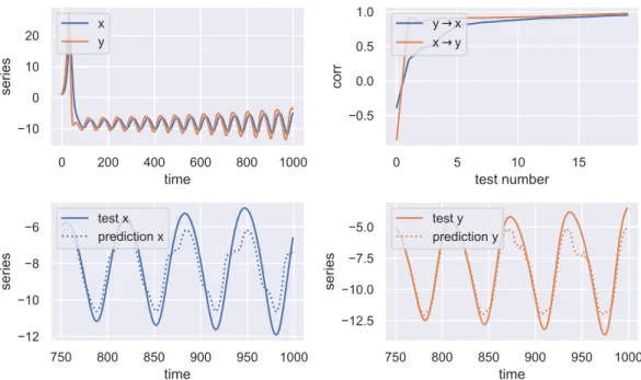
WLPH VHULHV [ \ WHVWQXPEHU FRUU \ [ [ \ WLPH VHULHV WHVW[ SUHGLFWLRQ[ WLPH VHULHV WHVW\ SUHGLFWLRQ\
Figure 4.3: CCM inference for the x and y coordinates of the Lorenz system.
4.5
Causal Chains
Inspired byMarkov chains (MC), we introduce a novel method in order to quantify sub-relations between causally linked state variables. Therefore, we begin with a simplified example of a four-dimensional system with state variables X1, X2, X3,
and X4. Their corresponding causality matrix is denoted as:
ψN ,N ≡ ψ1,1 ψ1,2 ψ1,3 ψ1,4 ψ2,1 ψ2,2 ψ2,3 ψ2,4 ψ3,1 ψ3,2 ψ3,3 ψ3,4 ψ4,1 ψ4,2 ψ4,3 ψ4,4 , (4.19)
whereψm,n ≥0denotes the direct causal influence ofXm onXnform, n∈ {1, . . . ,4}.
However, ψ1,2 for example does not incorporate the full causal influence of X1 on X2
since it only captures the direct influence. We identify other potential influences by constructing causal chains:
4.5. CAUSAL CHAINS 41 X1 ψ1,3 −−→ X3 ψ3,2 −−→ X2 X1 ψ1,4 −−→ X4 ψ4,2 −−→ X2 X1 ψ1,3 −−→ X3 ψ3,4 −−→ X4 ψ4,2 −−→ X2 X1 ψ1,4 −−→ X4 ψ4,3 −−→ X3 ψ3,2 −−→ X2, (4.20)
wherefore we introduce a set of rules:
• The chain stops when the system variable X2 is reached for the first time.
• We exclude loops: X1 ψ1,3 −−→ X3 ψ3,1 −−→X1 ψ1,3 −−→X3 ψ3,1 −−→. . .−−→ψ3,2 X2,
• We exclude recurring system variables:
X1 ψ1,4 −−→X4 ψ4,3 −−→X3 ψ3,1 −−→X1 ψ1,2 −−→X2,
where the system variable X1 appears twice.
Hence, we refer to the chains in equation 4.20 as causal chains of order O(1) since every system variable only appears once.
We quantify the causal influence of each chain using the geometric mean over the causality of each link, which in the simplified case yields:
c1 = (ψ1,3·ψ3,2) 1 2 c2 = (ψ1,4·ψ4,2) 1 2 c3 = (ψ1,3·ψ3,4·ψ4,2) 1 3 c4 = (ψ1,4·ψ4,3·ψ3,2) 1 3 . (4.21)
The geometric mean ensures that if one causal element in the chain is 0, the total causality for the chain diminishes as well.
Hence, we quantify the total causal influence of X1 on X2 as the mean over all
Ψ1,2 ≡ 1 nc nc X i=1 ci, (4.22)
with nc = 4 in the simplified case.
Extending this principle to anN-dimensional system, for one distinct pair(Xm, Xn)
the total number of causal chains is:
nc= N−2 X i=1 (N −2)! (N −i−2)!. (4.23)
This can easily be derived by building all possible sub-combinations between the system variables excluding the pair(Xm, Xn).
For all pairs(Xm, Xn), the total number of causal chains is given by:
Nc = N 2 ·nc= N! 2! · N−2 X i=1 1 (N−i−2)! . (4.24) Analogously, we define causal loops for equal pairs (Xn, Xn) to quantify the feedback
a state variableXn receives for a change of one unit.
In this case, the number of chains or loops for one variable is given by:
nl = N−1 X i=1 (N −1)! (N −i−1)!. (4.25)
In combination with causal chains, we can construct causality matrices by quantifying the causal link betweenXm andXn usingΨm,n instead ofψm,n. The resulting matrix
is denoted asΨN ,N with diagonal values quantifying the causal loop feedback. We
use the trace of the matrix in order to quantify the system causality:
ζ ψN ,N ≡ 1 N tr ΨN ,N . (4.26)
The attentive reader might have noticed that this definition violates the integrity condition specified in Section 4.1. However, we can solve this problem by setting the diagonal values to a constant value when constructing causality matrices.
Note that for a system of N = 3, this measure reduces to the geometric norm described in Subsection 3.2.3.
Chapter 5
Causality Driver Analysis
In this chapter we apply our model to identify and quantify linear and nonlinear drivers of causality in synthetic time series systems. To do so, we firstly compare the different inference techniques methodically using the coupled logistic system as a benchmark before applying them to the Lorenz attractor.
5.1
Measure Comparison
We compare GC, TE, and CCM regarding their causality evolution and robustness regarding window size, causal coupling, and noise. In this Subsection we conduct our analysis on the coupled logistic model specified in Subsection 2.2.1. The default parameters are chosen and the simulation length is set at T = 5000.
5.1.1
Evolution
We begin our analysis by calculating the causality evolutions over fixed-size sliding windows with size w= 1000and sliding delta δT = 200. We increase the robustness of our results by using K = 15 realizations of FT surrogates.
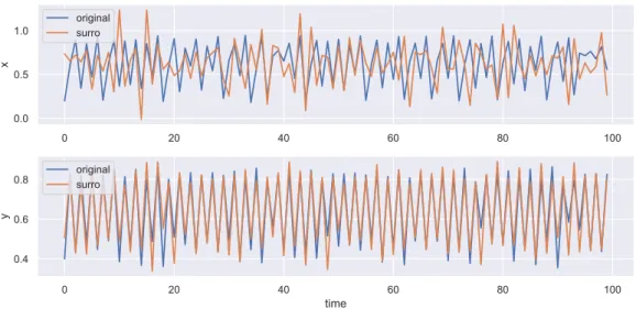
Pearson Correlation
In order to conduct a validity check of our model, we begin by evaluating the Pearson correlation. As discussed in Subsection 3.2.2, we expect the evolution of the correlation to be identical for the original and surrogate data. Furthermore, the cross measure evolutions are theoretically supposed to have a similar shape.
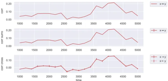
We observe in Figure 5.1 that our expectations are met and conclude that our surrogate generation is correct.
Due to the large size of our window, we do not explicitly measure the anti-correlation phases arising from mirage correlations mentioned in Subsection 2.2.1. However, we observe periods of different correlation strength.
FRUU [ \ FRUUVXUUR [ \ WLPH FRUUFURVV [ \ [ \
Figure 5.1: Pearson correlation in the coupled logistic system for fixed-size windows.
Mutual Information
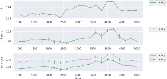
In order to ensure the correctness of our PDF estimation via histograms, we check whether the evolution of the surrogate MI has the same shape as the Pearson correlation.
For a bin size of nb = 75 and a bin range of rb = (0.005,0.995) we observe a high
similarity between the surrogate MI in Figure 5.2 and the Pearson correlation in Figure 5.1. This is numerically confirmed by a nested correlation of ρ= 0.93. Furthermore we find a high nested correlation ofρ= 0.89 between the surrogate MI and the cross MI from y to x. This indicates that the nonlinear part in x has no
contribution to the MI. This also applies to the other direction, for which the nested correlation has a lower value ofρ= 0.81.
We do however observe an increase of original MI between timestepst= 2500 and
t= 3500which is not present in the surrogate or cross data. We suggest the following interpretation: since the cross MI in both directions have very similar evolutions as the surrogate MI, for which the surrogatization is performed on both time series instead of one, this means that the nonlinear part in one time series has no strong
5.1. MEASURE COMPARISON 45
effect on MI. However, by comparing the evolutions to the original MI we see a significant difference. Hence, we can conclude that only the interaction between the nonlinearities of both time series affects MI while the nonlinearity of one single time series seems to be irrelevant.
Checking the additive nature between the MI evolutions did not generate findings that would warrant further studies.
PL [ \ PLVXUUR [ \ WLPH PLFURVV [ \ [ \
Figure 5.2: Mutual information in the coupled logistic system for fixed-size windows.
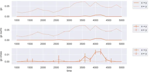
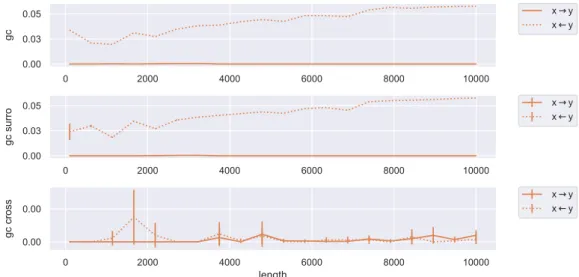
Granger Causality
As discussed in Section 4.2, GC measures solely the linear causality between time series. We observe this in Figure 5.3 by comparing the evolutions of the original and surrogate GC in both directions. We find them to be identical backed by a nested correlation of ρ= 0.99. Generally, the data indicates a higher linear causality from the x to the y coordinate and practically no causality the other way around. This is
inconsistent with the causal coupling chosen for the coupled logistic system. We will later find evidence that in this particular system, the causality from y to x is mainly
driven by nonlinearities and hence cannot be detected by GC.
Between time steps t= 3400and t = 4700we observe an increase in cross causality from x to y, which is also slightly present between t = 3800 and t = 4400 for the original and surrogate GC. We find that these artifacts arise from coherence phases of mirage correlations, which are detected as causality by GC.
Henceforth, we will mostly drop GC from our analysis since it offers no benefits for finding nonlinear causality drivers.
JF [ \ [ \ JFVXUUR [ \ [ \ WLPH JFFURVV [ \ [ \
Figure 5.3: GC in the coupled logistic system for fixed-size windows.
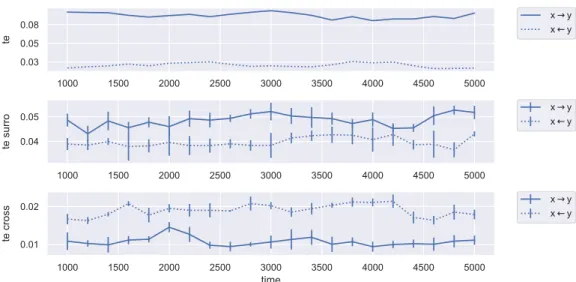
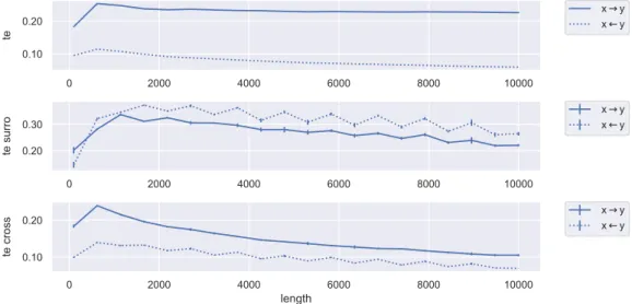
Transfer Entropy
In comparison to GC, TE incorporates both linear and nonlinear properties of causality in its inference. Analogously to MI, the bin size chosen is nb = 75 and the
bin range is set atrb = (0.005,0.995). Figure 5.4 illustrates the causality evolutions
detected by TE, which in contrast to GC, indicate a higher causality fromx to y for
both original and surrogate data. This is consistent with the causal coupling of the system. The cross causality further suggests that the causality from y to xis mainly
driven by linear properties iny.
We observe less fluctuation of the TE evolutions for the original data compared to the surrogate data. This can be interpreted as meaning that the total causal-ity consistently keeps the same level while the linear and nonlinear contributions fluctuate.
Even though GC theoretically is supposed to be the linear special case of TE, we do not find that the surrogate TE evolutions match with GC. Due to the difficulty with scoring GC, this was not to be expected. However, this calibration could be subject to further research in order to validate findings from analyses with TE.
Generally, we must note that the consistency of TE across original and surrogate data needs further research since TE appears to be very sensitive to the width of the distributions. Especially for the PDF estimation using histograms, we find that a sufficient resolution within the core ranges of the distributions is necessary for a robust estimation irrespective of the bin size. Preprocessing techniques such as rank-ordered remapping or rescaling described in Subsections 2.3.3 and 2.3.4 did not yield significant improvements.