Low-rank and sparse reconstruction in dynamic magnetic resonance imaging via proximal splitting methods

(1)

Low-rank and sparse reconstruction in

dynamic magnetic resonance imaging

via proximal splitting methods

Benjamin R. Tr´

emoulh´

eac

A dissertation submitted in partial fulfilment of the requirements for the degree of

Doctor of Philosophy of

University College London

Centre for Medical Image Computing Department of Computer Science

Department of Medical Physics and Biomedical Engineering

(2)

(3)

Declaration

I, Benjamin R. Tr´emoulh´eac, confirm that the work presented in this thesis is my own. Where information has been derived from other sources, I confirm that this has been indicated in the thesis.

Benjamin R. Tr´emoulh´eac December 2014

(4)

(5)

Abstract

Dynamic magnetic resonance imaging (MRI) consists of collecting multiple MR im-ages in time, resulting in a spatio-temporal signal. However, MRI intrinsically suffers from long acquisition times due to various constraints. This limits the full potential of dynamic MR imaging, such as obtaining high spatial and temporal resolutions which are crucial to observe dynamic phenomena.

This dissertation addresses the problem of the reconstruction of dynamic MR images from a limited amount of samples arising from a nuclear magnetic resonance experiment. The term limited can be explained by the approach taken in this thesis to speed up scan time, which is based on violating the Nyquist criterion by skipping measurements that would be normally acquired in a standard MRI procedure. The resulting problem can be classified in the general framework of linear ill-posed inverse problems. This thesis shows how dimensional signal models, specifically low-rank and sparsity, can help in the reconstruction of dynamic images from partial measurements. The use of these models are justified by significant developments in signal recovery techniques from partial data that have emerged in recent years in signal processing.

The major contributions of this thesis are the development and characterisation of fast and efficient computational tools using convex low-rank and sparse constraints via proximal gradient methods, the development and characterisation of a novel joint reconstruction–separation method via the low-rank plus sparse matrix decomposi-tion technique, and the development and characterisadecomposi-tion of low-rank based recovery methods in the context of dynamic parallel MRI. Finally, an additional contribution of this thesis is to formulate the various MR image reconstruction problems in the context of convex optimisation to develop algorithms based on proximal splitting methods.

(6)

(7)

Acknowledgement

I would like to thank my supervisors Simon Arridge and David Atkinson for their support and guidance. These years were a great opportunity to introduce me into academic research, in such a fascinating city that is London. I would like to ac-knowledge financial support from EPSRC. I’d like to thank both Dominique and Ron for making things easier in the lab. I would like to thank friends and colleagues at UCL, in particular Nikos, Uran, Luis, Elwin, Bjoern. My thoughts are also with Philip Batchelor.

On a more personal note, I am grateful to have met many lovely people in London. A special thank to David and Andrew for their support and friendship throughout these years. I also would like to thank the following Londoners: Alex, Aline, Antoine, Julie, Marin, Nathalie, Olivier, Romain, Yannick. I’d like to greet the formerguerriers, Étienne, Mathieu, Rémi, Flo, Julien and the rest of the team. Thanks to Dr. Alex for his advices, and thanks to my brother and his family. Finally, thanks to Diane for those moments you have shared with me, et évidemment, merci `

(8)

(9)

List of figures

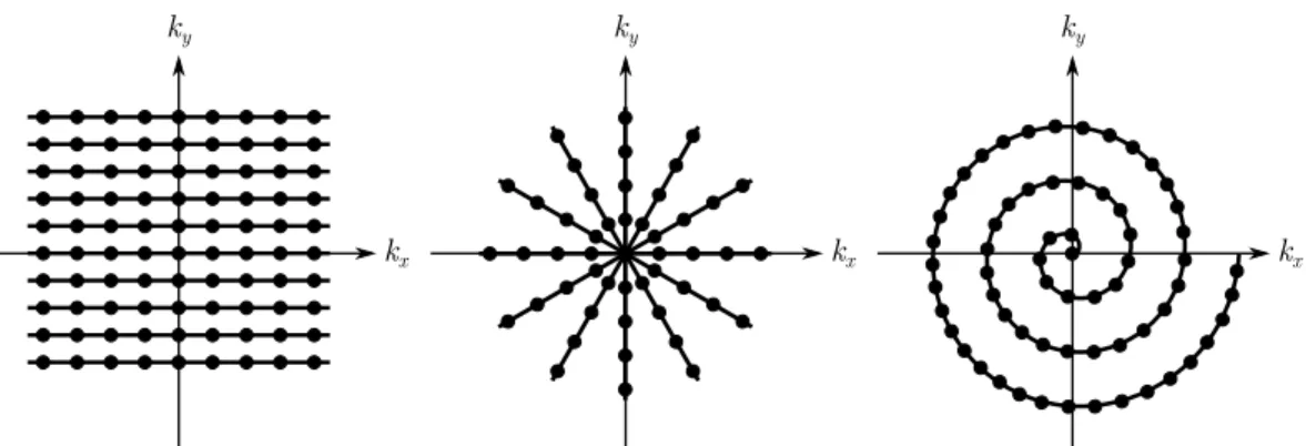
2.1 From left to right, standard Cartesian (rectilinear), radial and single shot spiralk-space trajectories in 2D. . . 44 2.2 Non-Cartesian sampling illustrated with two radial projections. The

problem is to generate uniform samples onto the Cartesian grid from nonuniformly spaced samples (black dots). . . 45 2.3 Dynamic magnetic resonance imaging. Left figure shows the k-space

in time, often referred to as (k, t)-space. Right figures represent com-mon dynamic imaging data: functional, cardiac and dynamic contrast enhanced MRI. . . 47

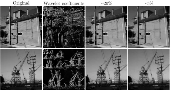
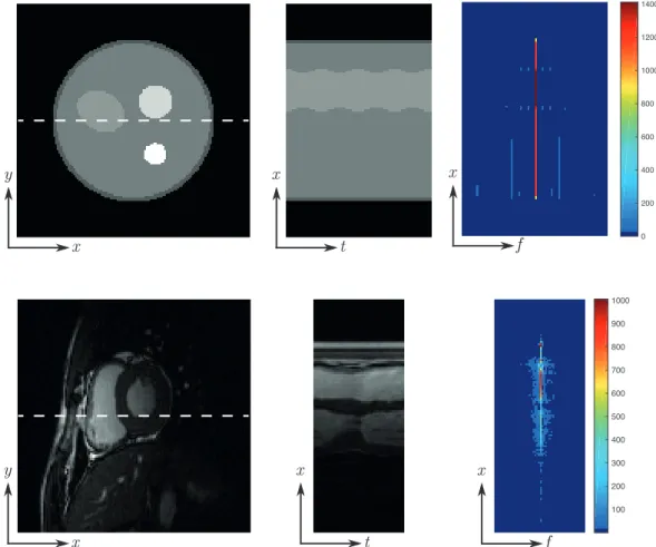
3.1 Two images converted into a sparse domain using a wavelet transform, and reconstructed with about 20% and 5% of their wavelet coefficients. 54 3.2 Illustration of the temporal Fourier transform for two typical dynamic

MRI datasets. Time frame images from the sequence (left), temporal profiles along the dashed lines (middle) and Fourier transform along the temporal direction resulting in sparse (x-f)-space signals (right). Note the specific colour mappings to highlight the sparsity. . . 68

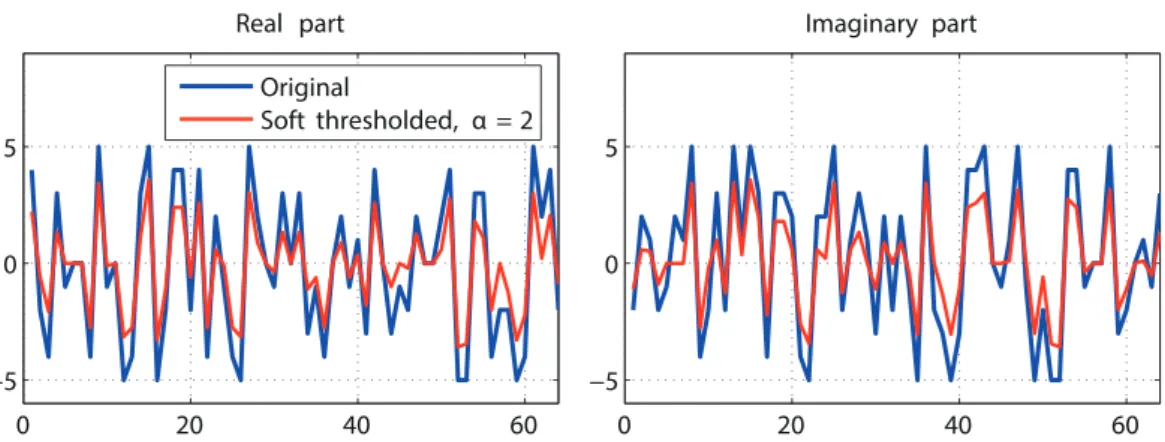
4.1 Graphs of functionsf(x) = 1₂(x−z)2+α|x|withα = 1 andz=−3 (blue), z = 0 (red) and z = 5 (green). Using the soft thresholding operator as defined in Eq. (4.7), we obtain Sr₁(−3) = −2, Sr₁(0) = 0 and Sr₁(5) = 4. . . 74 4.2 The soft thresholding operator applied on a complex-valued random

signal. The resulting signal (in red) is shrunk, hence the alternative ”shrinkage” name. . . 75 4.3 Convergence of algorithms. . . 85 4.4 Original sparse signal, minimum norm solution as in Eq. (3.3) and

the compressed sensing reconstructions (PG, FPG, ADMM). Both real and imaginary parts are shown as this is a complex-valued signal. 86

(14)

List of figures

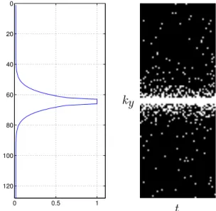
5.1 Polynomial variable density sampling pattern adapted for acquiring (k, t)-space samples. Left figure shows the probability density func-tion and right figure presents the (ky,t) sampling pattern. . . 95

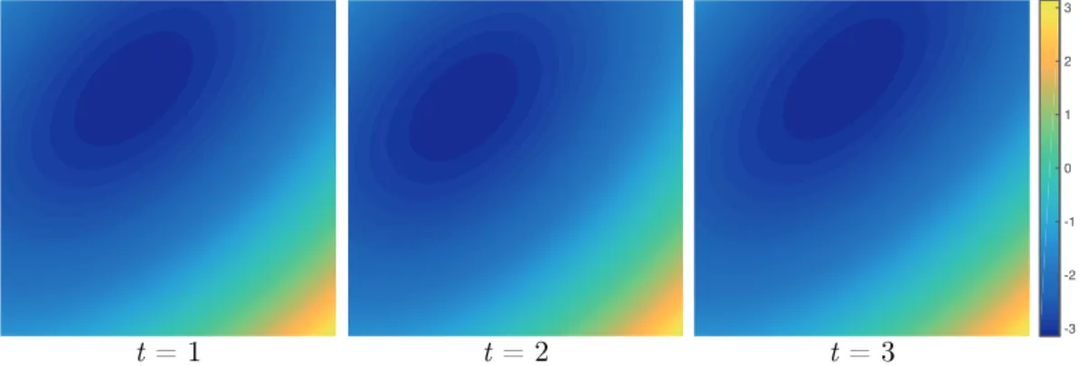
5.2 Equispaced and golden angle radial sampling with random rotations of the whole pattern for each time frame. . . 96 5.3 Spatially-smooth and slowly time-varying phase generated for three

time frames. . . 98 5.4 SL phantom showing magnitude (top) and phase (bottom) time frames

as well as associated x-t and y-t temporal profiles along the dashed lines. Left: noiseless, right: noisy. . . 98 5.5 PINCAT phantom showing magnitude (top) and phase (bottom) time

frames as well as associated x-t and y-t temporal profiles along the dashed lines. Left: noiseless, right: noisy. . . 99 5.6 Breath-hold cardiac dataset showing magnitude (left) and phase (right)

time frames as well as associatedx-t and y-t temporal profiles along the dashed lines. . . 99 5.7 Free-breathing cardiac showing magnitude (left) and phase (right)

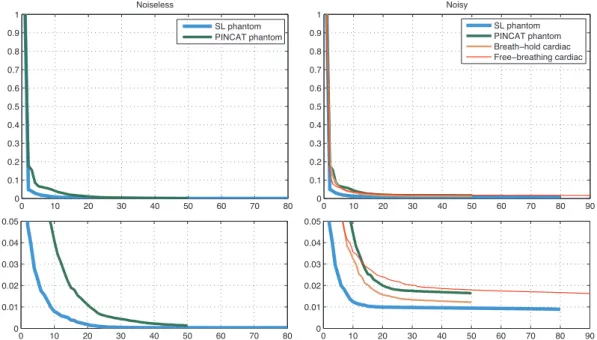
time frames as well as associatedx-t and y-t temporal profiles along the dashed lines. . . 99 5.8 Singular values (normalised) for the dynamic MRI datasets with

zoom-in graphs (bottom). . . 100 5.9 Intensity profiles along lines taken in the middle of the images. . . . 101 5.10 Sampling patterns used in this study, showing here only one

acqui-sition time frame. From left to right, PVD (Cartesian sampling), equispaced and golden angle radial sampling schemes. The red con-tours show the fully (or almost fully) sampled (k, t)-space sets that are used in k-t FOCUSS and PS-Sparse respectively to obtain the low-resolution estimate and to evaluate the basis for the temporal subspace. . . 101 5.11 Comparison of the different methods in terms of reconstruction

perfor-mance versus reconstruction time. Each point represents a computed reconstruction from table 5.2. Right figure is a close-up of the left figure. . . 102 5.12 Comparison of the different methods in term of reconstruction

perfor-mance versus computational time for SL phantom and PVD sampling. Right figure is a close-up of the left figure. . . 104 5.13 Normalised mean square error at each time frame for the different

datasets using equispaced angle radial sampling. . . 104 5.14 Singular values (normalised, zoom-in) for the different methods using

(15)

List of figures

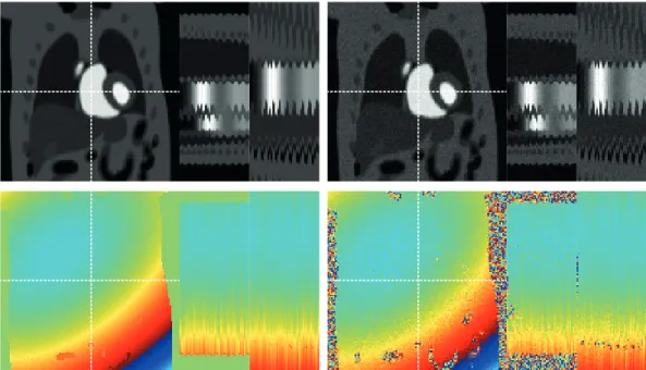
5.15 Error (×5) magnitude images for the SL phantom in the case of golden angle radial sampling. One frame and x-tand y-t profiles are shown for each method. . . 107 5.16 Reconstruction of the PINCAT phantom with equispaced angle

sam-pling. Top figures show extracted magnitude and phase images from the sequence. Bottom figures show x-t and y-tprofiles. . . 108 5.17 The influence of the sampling patterns with breath-hold cardiac

re-constructions and LRS-FCS algorithm. Left figures show magnitude and phase images extracted from the reconstructed sequences, right figure shows the NMSE. . . 109 5.18 Influence of randomness in time for radial-based sampling schemes. . 110 5.19 Extracted magnitude images from the reconstructed sequences (left),

and NMSE (right). Note the specific colour mapping to highlight the effect of blockwise SVT (pixels with zero value have a clearly distinct colour). . . 114 5.20 Influence of the regularisation parameters for the different methods,

showing here the SL phantom and golden angle radial sampling. . . 117

6.1 Schematic RPCA decomposition. Given a matrix X that is neither low-rank nor sparse, RPCA estimates low-rank L and sparse S ma-trices such thatX=L+S. . . 121 6.2 RPCA on a breath-hold cardiac cine MRI sequence with Nt = 30

(showing only a single frames from the sequence on the top figure). Algorithm 6.1 with ρ= 0.5 in Eq. (6.7) was used to generate figures in this example. The decomposition resulted in a rank-1 matrix for the low-rank part as shown by the only nonzero singular value, while the sparse component does not have a low rank because most of its singular values are not close to zero. It can be seen on the corre-sponding images and histograms that the sparse component is much more sparse than the low-rank one. . . 124 6.3 Effect of the additional temporal Fourier transform on the sparse

com-ponent using different decomposition parameterρ. Gray curve shows the normalised `1 norm of temporal Fourier transform of the sparse component (kF_t(S)k₁/kSk_F), black curve shows the normalised `1 norm of the sparse component (kSk1/kSkF). The additional

tempo-ral Fourier operator can genetempo-rally help sparsifying the signal when

S is not particularly sparse, e.g. ρ ∈ (0,1.2]. This figure has been generated using algorithm 6.1 and the numerical phantom with a combination of motion and intensity changes (section 6.3.2). . . 125

(16)

List of figures

6.4 (a) One time frame acquisition pattern for polynomial variable den-sity sampling and (b) the (ky, t)-space sampling pattern (left) with its

associated probability density function (right). (c) One time frame acquisition pattern for pseudo-radial sampling and (d) the (random) angles of rotation in time (left) with the associated uniform probabil-ity densprobabil-ity function (right). . . 129 6.5 Modelling local intensity changes (showing here pixel intensity values

in time) as the uptake and washout of a contrast agent using the modified Tofts model. . . 130 6.6 Qualitative results for phantom with a combination of intensity and

motion (Cartesian sampling). (a) Magnitude images (b) Zoom-in magnitude images (corresponding to the red square on the ground truth image) (c) Phase images (d) x-t temporal profiles and (e) y-t

temporal profiles (according to the dotted lines on the ground truth image). The time frames shown in the first three rows correspond to the frames selected on the dotted lines on the temporal profiles. Left color mappings refer to magnitude images, right color mapping refers to phase images. . . 131 6.7 (a,c) x-t temporal profiles and (b,d) y-t temporal profiles of various

reconstruction methods for (a,b) intensity only phantom and (c,d) motion only phantom (Cartesian sampling). . . 132 6.8 Visual comparison of reconstruction methods for cardiac MRI data

showing one time frame magnitude image (frame number n = 40). First row corresponds to Cartesian sampling, second row to pseudo-radial sampling. . . 135 6.9 NMSE at each time frame for cardiac MRI data with Cartesian

sam-pling (left) and pseudo-radial samsam-pling (right). . . 135 6.10 Different types of separation into low-rank and sparse components

using k-t RPCA with different decomposition parameters ρ. It can be observed that this parameter acts as a trade-off between the two components. The undersampling rate is 0.25. (a) Low-rank time frames (b) Sparse time frames (c) x-t temporal profiles of low-rank component (d) x-ttemporal profiles of sparse component. . . 137 6.11 x-ttemporal profiles used in the registration procedure. For the

reg-istration of k-t RPCA, only the low-rank part is used which mostly contains images without contrast enhancement (CE) thanks to the separation process. . . 138

(17)

List of figures

6.12 Displacement fields (zoom-in) over source images used for registra-tion. Table 6.5 provides the associated quantitative results. (a) Ground truth noiseless phantom (b) Noisy phantom with local in-tensity changes (c)k-tFOCUSS (d)k-tSLR (e)k-tRPCA, low-rank part. It can be seen that the displacement field is better estimated in the region with local changes of intensity ink-tRPCA. . . 139 6.13 Influence of regularisation parameters on the reconstruction error (in

dB) fork-tSLR andk-tRPCA. Numerical phantom simulations with 10-fold acceleration and Cartesian sampling. For k-t SLR, α and

β refers respectively to the nonconvex Schatten norm and spatio-temporal gradient. Fork-tRPCA,µ and ρ refers to (6.12). . . 140

7.1 The concept of dynamic parallel MRI illustrated with 4 coils (Nc= 4)

in the image domain (magnitude). For illustration purpose, sampling is at the Nyquist rate here but in practice it would be at sub-Nyquist rate and images would show artefacts. Each coil signal exhibit high correlation in time. SSoS stands for square root of sum of squares. . 147 7.2 Singular values of the unfolding modesX(q). These figures were

gen-erated with a signal of dimensions NxNy = 1282, Nt = 40, Nc = 16.

All unfolding modes have only a few significant singular values, al-though to different levels. Second row shows graphs in logarithmic scale. . . 151 7.3 The dynamic PMRI phantom used for numerical simulations with

artificially simulated sensitivity maps. Dimensions are Nx = Ny =

128, Nt= 40, Nc= 16. . . 152

7.4 Values of penalty terms (normalised) in the objective function (7.9) (low-rank tensor, left figure) and in the objective function (7.12) (local low-rank tensor with Ω = 64, right figure). . . 155

A.1 Unit balls for `p functions in R2 for various p. . . 167

A.2 Illustration of convex and nonconvex real-valued functions of one vari-able. For the strictly convex function (top left), the epigraph is shown in gray. . . 169

(18)

(19)

List of tables

4.1 Number of iterations, execution times and absolute reconstruction errors for the CS algorithms. . . 85

5.1 Sparsity characterisation of the different datasets. Right column rep-resents the decreasing amount of sparsity in percentage, e.g. the PINCAT phantom benefits most from the temporal Fourier transform. 100 5.2 Quantitative reconstruction results (in dB). . . 103 5.3 Reconstruction results (in dB) using Eq. (B.2) for low-rank

regu-larisation via convex, nonconvex and hard thresholding approaches. ZF-IDFT reconstructions are reported for reference. . . 112

6.1 Characteristics of the different noiseless phantoms. The spatio-temporal TV operator is computed as defined in Eq. (3.62). . . 133 6.2 Reconstruction results (in dB) using Eq. (B.2) for numerical

phan-toms with Cartesian sampling. Numbers in brackets refer to regular-isation parameters. . . 134 6.3 Reconstruction results (in dB) using Eq. (B.2) for numerical

phan-toms with pseudo-radial sampling. Numbers in brackets refer to reg-ularisation parameters. . . 134 6.4 Reconstruction results (in dB) using Eq. (B.2) for cardiac MRI data

with Cartesian and pseudo-radial sampling. . . 135 6.5 Displacement fields results in the region of interest with local intensity

changes. Quantities are in dB and have been computed using the Jacobian and Eq. (B.2). . . 139

7.1 The third-order tensor Xand its mode-q unfolding X(q). . . 150 7.2 Reconstruction results (in dB) using Eq. (B.2). Note thatk-tSENSE,

k-t SPARSE-SENSE andk-t low-rank SENSE require an estimation of the coil sensitivity profiles, in contrast to by-coil sparse, coil-by-coil low-rank and low-rank tensor reconstructions that make use of implicit coil sensitivities. The notationα1,2,3= 10 means that α1,

(20)

List of tables

7.3 Reconstruction results (in dB) using Eq. (B.2) for locally low-rank tensor recovery withα1=α2 =α3 = 10 and different Ω. . . 155

(21)

List of algorithms

4.1 Compressed sensing MRI via proximal gradient . . . 83 4.2 Compressed sensing MRI via fast proximal gradient . . . 83 4.3 Compressed sensing MRI via alternating direction method of multipliers 84 5.1 Sparse signal recovery via fast proximal gradient (S-FPG) . . . 92 5.2 Low-rank matrix recovery via fast proximal gradient (LR-FPG) . . . 93 5.3 Low-rank matrix and sparse signal recovery via fast composite

split-ting (LRS-FCS) . . . 94 5.4 Low-rank matrix and sparse signal recovery via generalised

forward-backward splitting (LRS-GFBS) . . . 94 5.5 Local low-rank matrix recovery via fast proximal gradient (LLR-FPG) 113 6.1 Robust principal component analysis (RPCA) . . . 122 6.2 Dynamic MR image reconstruction–separation via low-rank plus sparse

prior (k-tRPCA) . . . 128 7.1 Low-rank tensor recovery for dynamic parallel MR imaging via fast

(22)

(23)

List of acronyms and

abbreviations

2D Two-dimensional

ADMM Alternating direction method of multipliers

AL Augmented Lagrangian

ALM Augmented Lagrangian method

CS Compressed sensing

CT Computed tomography

dB Decibel

DCE Dynamic contrast-enhanced

DFT Discrete Fourier transform

FCS Fast composite splitting

FISTA Fast iterative shrinkage-thresholding algorithm

FFT Fast Fourier transform

FOV Field of view

FPG Fast proximal gradient

GFBS Generalised forward-backward splitting

i.i.d. Independent and identically distributed

IDFT Inverse discrete Fourier transform

MM Method of multipliers

MR Magnetic resonance

MRI Magnetic resonance imaging

NMR Nuclear magnetic resonance

NMSE Normalised mean square error

PCA Principal component analysis

PMRI Parallel magnetic resonance imaging

PVD Polynomial variable density

RF Radio frequency

RIP Restricted isometry property

RPCA Robust principal component analysis

(24)

List of acronyms and abbreviations

SNR Signal-to-noise ratio

SSoS Square root of sum of squares

SVD Singular value decomposition

(25)

List of symbols

Common symbols

i Imaginary unit

<,= Real part, imaginary part

.>,.H Transpose, conjugate transpose

¯. Complex conjugate .∗ Adjoint .? Optimal point b. Estimation N Normal distribution ∂ Partial derivative α, β, µ, λ ∈R+ Regularisation parameters ρ ∈_R+ ∗ Step size L ∈_R+ ∗ Lipschitz constant

δK, δR ∈R+ Isometry constants forK-sparse signal andR-rank matrix

δ ∈_R+ _{Penalty parameters for augmented Lagrangian} ˆ_i_,ˆ_j_,_kˆ _∈_R3 _{Unit vectors in the Cartesian coordinate system}

D ∈ {1,2,3} Signal dimension for continuous data

r ∈_RD _{Position coordinates for continuous data}

k ∈_RD _k_{-space coordinates for continuous data}

Functions

S,Sj ∈C k-space function, k-space function for coilj

Γj ∈C Sensitivity map for coilj

I ∈_C Image function

E ∈C Encoding function

N ∈_C Noise function

F ∈_R Objective function

L,LA _∈

R Lagrangian function, augmented Lagrangian function

(26)

List of symbols

Discrete data

N, M, N1, N2, . . . ∈N Vector or matrix dimension

Nx ∈N Number of pixels for x-coordinate

Ny ∈N Number of pixels for y-coordinate

Nt ∈N Number of temporal frames

Nc ∈N Number of coils

y ∈CM k-space measurement vector

n ∈_CM _{Noise vector}

I ∈_RN×N _{Identity matrix}

A ∈RM×N Sampling matrix

Ψ ∈_CN×N _{Sparsifying transform matrix}

F ∈_CN×N _{Fourier transform matrix}

E ∈CM×N MRI encoding matrix

X ∈_CN1×N2×...×NQ _Q_{-order tensor}

Operators

A Sampling operator

Ψ Sparsifying transform operator

F Fourier transform operator

Ft Temporal Fourier transform operator

E MRI encoding operator

EΓ Parallel MRI encoding operator

prox_g Proximal operator ofg

∇ Gradient operator

S CN →CN Soft thresholding operator [Eq. (4.11)]

Sp

CN →CN Generalised soft thresholding operator [Eq. (5.14)]

H CN →CN Hard thresholding operator [Eq. (4.52)]

SVTS CM×N →CM×N Singular values soft thresholding operator [Eq. (4.14)]

SVTSp CM×N →CM×N Singular values generalised soft thresholding operator

[Eq. (5.15)]

SVTH CM×N →CM×N Singular values hard thresholding operator

(27)

Chapter 1 Introduction

Contents

1.1 Motivations . . . 27 1.2 Problem statement . . . 28 1.3 Thesis objectives and contributions . . . 29 1.4 Outline . . . 30

1.1 Motivations

Seeing inside the living body without the need for exploratory surgery has always been a challenge in human history. This has been possible since X-rays were discov-ered in 1895 by R¨ontgen, who produced the first picture showing bone structures of his wife’s hand. From that time, a number of medical imaging techniques have been developed, such as positron emission tomography, X-ray computed tomography (CT), nuclear magnetic resonance imaging or ultrasound.

Nuclear magnetic resonance imaging, or simply magnetic resonance imaging (MRI), is a medical imaging technique that is based primarily upon the sensitiv-ity to the presence and properties of water. MRI uses magnetic fields and radio electromagnetic waves to detect tiny changes in the magnetism of the nucleus of the hydrogen atom which is found in abundance in the human body. MRI is a valu-able diagnostic tool that is extensively used in radiology to examine the anatomy and physiology of the body. It is generally regarded as a safe procedure because it does not involve ionising radiation in contrast to X-ray CT for example. MRI can also produce different types of images without any mechanical modification to the MRI scanner, such as different image contrasts or images of the subject in various orientations and positions.

In this thesis, we are interested in dynamic MRI, a technique that consists of collecting MR images in time and thus generating a spatio-temporal signal. Dynamic

(28)

Introduction

MRI is used in multiple clinical applications, such as cardiovascular (or cardiac) MRI, dynamic contrast-enhanced (DCE) MRI or functional MRI (fMRI). Cardiac MR imaging is used to capture and study quantitative assessment of the heart. A primary application is cine cardiac imaging, which assesses both structure and function of the beating heart. Other applications include for example myocardial perfusion imaging to detect coronary artery disease or phase contrast imaging to quantify blood flow velocity through the heart. Regarding DCE MRI, it is used to assess the passage and distribution of a contrast agent through organs and may possibly be used as a source of biomarkers in oncology. An important example is breast cancer imaging based on gadolinium contrast agent. In neuroimaging studies, functional MRI is used to localise brain activities by detecting blood-oxygen-level-dependent signals.

However, one of the fundamental limiting factor of MRI is its serial acquisition procedure that is inherently slow due to various constraints. These include intrin-sic nuclear relaxation times that generate the signal to acquire, how fast gradient magnetic fields can be switched on and off without causing peripheral nerve stim-ulations, how fast the oscillating radio frequency magnetic field can be turned on and off to prevent tissue heating (specific absorption rate), and signal-to-noise ratio constraints. Although it is possible to image static objects such as the brain with a slow acquisition procedure, it is much more problematic to collect images of moving structures such as the beating heart or in which contrast changes over time, as in dynamic MR imaging.

This thesis is motivated by the benefits of reducing the acquisition time of dy-namic MRI while maintaining the image quality. From the patient perspective, it increases comfort, facilitates scans for problematic subjects such as the very young, old or ill, and also limits patient exposure to magnetic fields and acoustic noise. From an imaging aspect, obtaining faster scan times can benefit every dynamic MRI appli-cations mentioned previously, since higher temporal resolution better characterises dynamic processes, or trading the time saving for higher spatial resolution provides greater anatomical details. Minimisation of the patient’s time in the scanner also decreases the chances of motion artefacts such as blurring in the resulting images.

1.2 Problem statement

The main problem addressed in this thesis is the reconstruction of spatio-temporal magnetic resonance images from a limited amount of samples acquired in the Fourier domain, known as (k, t)-space in MRI. The term limited can be explained by the approach taken in this thesis to speed up scan time, which is based on violating the Nyquist criterion by skipping measurements that would be normally acquired in a standard MRI procedure.

(29)

Thesis objectives and contributions

Due to the physics of MRI, the spatio-temporal MRI signalS(k, t) can be mod-elled mathematically through the Fourier integral as

S(k, t) =

Z

I(r, t)e−i2π(r·k)dr+N(k, t), (1.1)

whereI(r, t) andN(k, t) are respectively the spatio-temporal image and noise func-tions, andkandrare respectively thek-space and position coordinates. The image reconstruction task can be expressed as: given a finite set of sub-Nyquist Fourier measurements from Eq. (1.1), find the best discrete approximation of the spatio-temporal function I(r, t). This represents a typical example of a linear ill-posed inverse problem.

1.3 Thesis objectives and contributions

This thesis shows how incorporating prior information based on low-dimensional signal models can help in the reconstruction of spatio-temporal images from a limited amount of Fourier samples arising from a nuclear magnetic resonance experiment.

More specifically, this thesis investigates the use of low-rank and sparse signal models throughproximal splitting methods to help in the reconstruction ofdynamic MR images from partial data. Low-rank and sparsity models have contributed to significant developments in signal recovery techniques in recent years in the fields of signal processing and applied mathematics. These models can be classified as low-dimension or low-complexity as they are related to the principle of parsimony, also known as Occam’s razor, which states that the simplest among competing hy-potheses should be preferred. The use of proximal splitting methods in this thesis are encouraged by the requirement of reconstruction algorithms (i) to handle nons-mooth penalties due to low-rank and sparse constraints, and (ii) to tackle relatively large-scale problems due to spatio-temporal MR signals lying in high-dimensional spaces. This thesis aims to provide an adequate trade-off between the theoretical concepts of signal recovery and the practical aspects of the MRI reconstruction prob-lem from limited Fourier measurements. In short, the major contributions of this thesis are

• the development and characterisation of computational methods for low-rank and sparsity constrained problems based on fast proximal gradient methods,

• the development and characterisation of a joint reconstruction–separation model that goes beyond traditional reconstruction methods,

• the development and characterisation of low-rank based recovery methods in combination with sub-Nyquist dynamic parallel MR imaging,

(30)

Introduction

• the formulation of the various MR image reconstruction problems in the con-text of convex optimisation and proximal splitting methods.

These contributions are further explained in section 1.4 which presents the outline of this manuscript. Some of the work presented in this thesis have been previously published in journal article:

• B. Tr´emoulh´eac, N. Dikaios, D. Atkinson, and S. R. Arridge. Dynamic MR image reconstruction–separation from undersampled (k,t)-space via low-rank plus sparse prior. IEEE Transactions on Medical Imaging, 33(8):1689–1701, 2014.

And in international conference papers:

• B. Tr´emoulh´eac, D. Atkinson, and S. R. Arridge. Low-rank and (x-f)-space sparsity via fast composite splitting for accelerated dynamic MR imaging. In

Proceedings of IEEE International Symposium on Biomedical Imaging (ISBI), pages 649–652, Beijing, 2014.

• B. Tr´emoulh´eac, D. Atkinson, and S. R. Arridge. Fast dynamic MRI via nuclear norm minimization and accelerated proximal gradient. InProceedings of IEEE International Symposium on Biomedical Imaging (ISBI), pages 322– 325, San Francisco, 2013.

• B. Tr´emoulh´eac, D. Atkinson, and S. R. Arridge. Motion and contrast en-hancement separation model reconstruction from partial measurements in dy-namic MRI. In Proceedings of Medical Image Computing and Computer As-sisted Intervention (MICCAI) Workshop on Sparsity Techniques in Medical Imaging, Nice, 2012.

Work during this thesis has also resulted in other publications as co-author in inter-national conferences, although not reported in this manuscript.

1.4 Outline

The necessary background on magnetic resonance imaging is introduced in chapter 2. We take care of describing the MRI signal path from the most simplest raw nuclear magnetic resonance signal (nuclear magnets) to arrive at the Fourier integral transform. Other important topics covered include image reconstruction, noise issues and dynamic MR imaging.

Chapter 3 describes linear inverse problems, a fundamental topic not only in medical imaging but in many other areas of science and engineering. Most of this chapter is concerned with signal recovery from partial data. We emphasise the

(31)

Outline

description of signal recovery methods through the use of low-dimensional signal models that have gained much interest in the past decade. We then discuss state of the art recovery techniques for the specific problem of dynamic MRI reconstruction. Chapter 4 introduces succinctly proximal splitting methods, a general optimi-sation framework that provides efficient and flexible algorithms to minimise certain types of convex problems. This framework forms the basis to solve the different formulated image reconstruction problems in this thesis.

Chapter 5 develops and characterises efficient computational tools based on prox-imal gradient for MR image reconstruction that exploits sparse and low-rank struc-tures. Characterisation of these methods are shown with multiple realistic datasets and various comparisons with other state of the art methods.

Chapter 6 proposes a joint reconstruction–separation model that goes beyond traditional reconstruction methods from partial observations. The model is based on the low-rank plus sparse matrix decomposition to both regularise and intrinsically separate reconstructed dynamic data. The proposed technique provides a competi-tive reconstruction method, as well as the ability to separate clinically-relevant data in the context of dynamic contrast enhanced MRI.

In chapter 7, we explore low-rank based recovery approaches in combination with dynamic parallel imaging. Parallel imaging is the most widely used technique to accelerate imaging scan in clinical practice. We show how low-rank based signal recovery techniques can be combined with dynamic parallel imaging in various ways to enable further improvement in image reconstruction.

We conclude this thesis in chapter 8 by providing a summary of contributions, the current limitations and perspectives of this thesis.

(32)

(33)

Chapter 2 Principles of magnetic

resonance imaging

Contents

2.1 Introduction . . . 33 2.2 Nuclear magnetic resonance phenomenon . . . 34 2.3 Signal detection . . . 36 2.4 Spatial localisation . . . 39 2.5 Fourier encoding . . . 40 2.6 Image reconstruction . . . 41 2.6.1 Sampling . . . 42 2.6.2 Algebraic formulation . . . 44 2.6.3 Cartesian and non-Cartesian sampling . . . 44 2.7 Noise . . . 46 2.8 Dynamic imaging . . . 47 2.9 Conclusion . . . 48

2.1 Introduction

In this chapter, fundamental concepts of magnetic resonance imaging (MRI) are presented. Due to the complicated nature of an MRI system however, we only present an overview of the physics of MRI. The reader is referred to Refs. [1–3] for a more in-depth analysis.

This chapter is organised as follows. We discuss the nuclear magnetic resonance (NMR) phenomenon in section 2.2. The concepts of signal detection, spatial locali-sation and Fourier encoding are then described respectively in sections 2.3, 2.4 and

(34)

Principles of magnetic resonance imaging

2.5. Note that from section 2.2 to 2.5, we describe consecutively the various forms and transitions of the MRI signal as

µ−→M−→M+(t)−→V(t)−→S(t)−→S(k),

where µrepresents the nuclear magnetic moment, M an ensemble of spins, M+(t) the transverse magnetisation, V(t) the voltage signal, S(t) the nuclear magnetic resonance signal, to finallyS(k) the k-space signal. The transition from continuous to discrete data is then explained in the image reconstruction section 2.6. Noise in MRI is discussed in section 2.7, dynamic imaging in section 2.8 and we conclude this chapter in section 2.9.

2.2 Nuclear magnetic resonance phenomenon

MRI relies on the nuclear magnetic resonance (NMR) phenomenon which involves the interaction of atomic nuclei in a magnetic field. It was first observed indepen-dently by Bloch and Purcell in 1946 for which they shared the Nobel Prize in Physics in 1952. To understand the NMR phenomenon, we should in principle start at the nuclear level using laws of quantum theory because the behaviour of atomic and subatomic particles can only be accurately described in this framework. However, the phenomenon can be explained more simplistically using the theory of classical (Newtonian) mechanics. It is possible to do so because MRI deals with the collective behaviour of a large ensemble of particles.

Atoms consist of nuclei (protons and neutrons) surrounded by their orbiting electrons. A nucleus has a finite radius, mass and a net electric charge. Some nuclei, depending on their atomic weights or numbers, possess an angular momentum

J often called spin, such as the nucleus of the hydrogen atom present in water. This angular momentum combined with the electric charge of the nucleus induces a magnetic field known as the nuclear magnetic moment µ. The nuclear magnetic moment can be expressed as

µ=µxˆi+µyˆj+µzkˆ, (2.1)

where (ˆi,ˆj,kˆ) denote the unit directional vectors in the standard Cartesian coordi-nate system and (µx, µy, µz) the scalar components of µ. The angular momentum

and the magnetic moment are related via µ=γJ, where γ is a nucleus dependent constant known as thegyromagnetic ratio. Nuclei with nonzero µare then regarded as microscopic magnets. Nuclear spin can be visualised as a physical rotation of the nucleus about its own axis, although it is a property characterised by quantum mechanics.

(35)

Nuclear magnetic resonance phenomenon

total magnetic fieldM is referred to as thebulk magnetisation vector,

M=X

n

µ_n=Mxˆi+Myˆj+Mzkˆ, (2.2)

where the nth nucleus has magnetic moment µ_n. Magnitudes of each magnetic moment |µ_n| are known under any conditions, but their directions are completely random due to thermal movements. This results in no net magnetisation,M=0.

However, in the presence of an external magnetic field applied in the z-direction

B0 = B0kˆ, nuclear magnetic moments for the hydrogen are restricted to two pos-sible orientations: parallel to B0 (alignment, spin up) or antiparallel to B0 (anti-alignment, spin down). On average, more nuclear spins align with the magnetic field than against, which results in a net bulk thermal equilibrium magnetisation in the

z-direction

M=M_z0kˆ (2.3)

whereM_z0 represents the thermal equilibrium value for Min the presence of B0. Apart from forcing them to align, each magnetic moment experiences a torque from B0 causing it to precess about the ˆk axis. This phenomenon is callednuclear

precession and can be physically interpreted as the wobbling of a spinning-top about the gravitational axis, or the precession of a spinning toy gyroscope. The precession frequency of µexperiencing aB0 field is given by the Larmor equation

ω0 =γ|B0|=γB0. (2.4)

We consider now an oscillating magnetic fieldB1in addition to the staticB0field. (The strength of B1 is much weaker than B0.) The application of this oscillating magnetic field causes M to tip away from the B0 field at a specific angle, known as the flip angle. The B1 field is often referred to as radio frequency (RF) pulse because it oscillates in the radio frequency range and it is turned on only for a few milliseconds. The resonance condition in magnetic resonance imaging is that

B1 should rotate in the same manner as the precessing spins, i.e. rotating at the Larmor frequencyω0 around the z-direction.

In the presence of the external magnetic field B1(t), the time-dependent be-haviour of the bulk magnetisation vectorMcan be described according to the Bloch equation ∂M ∂t =γM×B− 1 T2 (Mxˆi+Myˆj) + 1 T1 (M_z0−Mz)ˆk, (2.5)

whereB=B0+B1(t) is the total magnetic field experienced by the nuclei;T1andT2 are decay constants called relaxation times that characterise the relaxation process after the spin system has been perturbed (they depend on the different tissues such as white/grey matter or fat); andM_z0 is the thermal equilibrium value forMin the

(36)

presence ofB0 only.

According to the laws of thermodynamics, and provided the RF pulse is turned off and sufficient time is given, the spin system relaxes back towards its original equilibrium state. This phenomenon is called relaxation and is characterised by a precession of M about the B0 field, a recovery of the longitudinal magnetisation

Mz (longitudinal relaxation) and the destruction of the transverse magnetisation

M+ (transverse relaxation). From the solutions to the Bloch equation, the time evolution for the longitudinal and transverse magnetisations are

Mz(t) =Mz0(1−e

−t/T1_{) +}_M

z(0)e−t/T1, (2.6a)

M+(t) =M+(0)e−t/T2e−iω0t, (2.6b)

where Mz(0) and M+(0) are respectively the magnetisation along the z-direction and on the transverse plane after an RF pulse. The transverse relaxation M+ uses the complex representation

M+(t) =Mx(t) +iMy(t), (2.7) with Mx(t) =e−t/T2 Mx(0) cos(ω0t) +My(0) sin(ω0t) , My(t) =e−t/T2 My(0) cos(ω0t)−Mx(0) sin(ω0t) . (2.8)

The complex formulation is useful because the main activity of the spin in a static magnetic field is a rotation in the 2D transverse plane.

2.3 Signal detection

Signal detection relies on the Faraday law of electromagnetic induction. This law states that a time-varying magnetic flux Φ(t) (in Webers) through an electric circuit produces an electromagnetic forceE(t) (in Volts). More specifically, the electromag-netic force E(t) induced in the circuit is equal to the negative of the time rate of change of the magnetic flux,

E(t) =−∂Φ(t)

∂t . (2.9)

According to the principle of reciprocity, the magnetic flux in MRI can be expressed as

Φ(t) =

Z

Br(r)·M(r, t)dr, (2.10)

where Br(r) = B_xr(r)ˆi+B_yr(r)ˆj+B_zr(r)ˆk is the magnetic field received in the coil and M(r, t) is the bulk magnetisation vector, both at position r = xˆi+yˆj+zˆk.

(37)

Signal detection

Hence, the electromagnetic force is given by

E(t) =−∂

∂t

Z

Br(r)·M(r, t)dr. (2.11)

The voltage signal V(t) induced in the MRI system coil is proportional to Eq. (2.11) depending on the characteristics of the measurement system. Explic-itly, it can be written as

V(t)∝ −∂ ∂t Z B_xr(r)Mx(r, t) +Bry(r)My(r, t) +Bzr(r)Mz(r, t) dr. (2.12)

To develop expression (2.12), first note that the previous static-field solutions (2.6a) and (2.6b) hold for eachr,

Mz(r, t) =Mz0(1−e−t/T1(r)) +Mz(r,0)e−t/T1(r), (2.13a)

M+(r, t) =M+(r,0)e−t/T2(r)e−iω0t=|M+(r,0)|eiφ0(r)e−t/T2(r)e−iω0t, (2.13b)

where the phaseφ0and magnitude|M+(r,0)|are determined by the initial RF pulse conditions in Eq. (2.13b). We now address the computation of the time derivatives in Eq. (2.12). For ∂tMz, we have

∂Mz(r, t) ∂t = ∂ ∂t M_z0(1−e−t/T1(r)) +Mz(r,0)e−t/T1(r) =e−t/T1(r) M 0 z T1(r) −Mz(r,0) T1(r) . (2.14)

For∂tMx and∂tMy, it is useful to employ the complex representation (2.7) with the

fact that Mx =<{M+}and My =={M+},

∂Mx(r, t) ∂t = ∂<{M+(r, t)} ∂t =< n∂ ∂tM+(r,0)e −t/T2(r)_e−iω0to =−<nM+(r,0) 1 T2(r) +iω0 e−t/T2(r)e−iω0to, (2.15) ∂My(r, t) ∂t = ∂={M+(r, t)} ∂t =−= n M+(r,0) 1 T2(r) +iω0 e−t/T2(r)e−iω0to. (2.16)

However, since the Larmor frequency ω0 is generally orders of magnitude larger than typical values of 1/T1 and 1/T2, the time derivatives ∂tMx and ∂tMy can be

approximated to

∂tMx(r, t)≈ −ω0e−t/T2(r)<{iM+(r,0)e−iω0t}, (2.17a)

(38)

and expression (2.12) can be simplified to

V(t)∝ − Z B_xr(r)∂tMx(r, t) +Bry(r)∂tMy(r, t) dr. (2.18)

The above expression shows that the dominant signal induced in the receiver coil is due to the transverse magnetisation and not the longitudinal magnetisation. Sub-stituting the approximated derivatives (2.17a) and (2.17b) into (2.18) yields

V(t)∝ω0 Z e−t/T2(r) B_xr(r)<{iM+(r,0)e−iω0t}+Byr(r)={iM+(r,0)e−iω0t dr. (2.19) Using the fact thatM+(r,0) =|M+(r,0)|eiφ0(r) from Eq. (2.13b), the above expres-sion reads V(t)∝ω0 Z e−t/T2(r)|M+(r,0)| B_xr(r) sin(ω0t−φ0(r)) +Bry(r) cos(ω0t−φ0(r)) dr. (2.20) This expression can be further simplified to

V(t)∝ω0

Z

|B₊r(r)||M+(r,0)|e−t/T2(r)sin(ω0t+φr(r)−φ0(r))dr (2.21)

by defining the magnetic field received components as

B_xr(r) =|B₊r(r)|cos(φr(r)), (2.22a)

B_yr(r) =|B₊r(r)|sin(φr(r)), (2.22b)

whereφr(r) is the reception phase angle.

At this stage, V(t) is a high-frequency signal because the transverse magneti-sation vector precesses at the Larmor frequency ω0, which is about 42.5 MHz per Tesla for hydrogen protons. To avoid potential problems in later stages, this signal is moved to a low-frequency band in order to be free of the high Larmor oscillation. In practice, it consists of multiplying the time signalV(t) by a complex exponential with frequency Ω = ω0 +δω where δω is a small offset frequency, or equivalently multiplyingV(t) separately with a cosine and sine signals at the frequency Ω. Each separate signal then results in two components, one close to the offset frequency and the other nearly twice the Larmor frequency. Both signals are then low-pass filtered to remove frequency around (2ω0 +δω), resulting in signals oscillating only at the offset frequency δω. This procedure is calledquadrature detection and the outputs of such technique are two demodulated and filtered signals denotedVP(t) andVQ(t), oscillating at frequency aroundδω, that are put together in complex form

(39)

Spatial localisation

where VP represents the in-phase signal (real part) and VQ the quadrature signal (imaginary part). After quadrature detection, the resulting NMR signal can be expressed as

S(t)∝ω0

Z

|Br₊(r)||M+(r,0)|e−t/T2(r)e−i(δωt+φr(r)−φ0(r))dr. (2.24)

From Eqs. (2.13b) and (2.22), we have

M+(r,0) =|M+(r,0)|eiφ0(r), (2.25a) ¯

B₊r(r) =|B₊r(r)|e−iφr(r)_, _(2.25b)

where ¯B₊r denotes the complex conjugate ofB₊r. Eq. (2.24) can be further simplified to

S(t)∝ω0

Z

¯

Br₊(r)M+(r,0)e−t/T2(r)e−iδωtdr. (2.26)

Eq. (2.26) is here a function of T2 only but the use of different combinations of RF pulses and gradient fields can condition the signal to be a function of the proton density, T1 relaxation,T2 relaxation, T2∗ relaxation and several other tissue proper-ties.

2.4 Spatial localisation

Spatial localisation refers to applying additional spatial and time-varying magnetic fields on top of the static magnetic field, to allow spins to be excited at different frequencies at different locations, and hence making possible the representation of an object that is spatially inhomogeneous. These magnetic fields are referred to as

gradient magnetic fields or simply as gradients. The use of gradients to spatially encode information was first proposed by Lauterbur in 1973 [4].

The first step of spatial localisation is to select the slice by using a gradient in the z-direction, referred to as slice selective gradient and denoted Gz. Once the

RF pulse has been made spatially slice selective, the rest of the process is in-plane localisation and known as spatial encoding. This is achieved with a phase-encoding

gradient in the y-direction (Gy) and a frequency-encoding (or read-out) gradient in

thex-direction (Gx).

By defining the offset frequencyδω=γ(Gxx+Gyy+Gzz) (withγ the

gyromag-netic ratio) in Eq. (2.26), it yields

S(t)∝ω0

Z

¯

(40)

Furthermore, if we introduce the vector notation

k(t) = γ 2π    Gxt Gyt Gzt   = γ 2π Gxtˆi+Gytˆj+Gztˆk , (2.28)

we can write the final expression as

S(k)∝ω0

Z

¯

B₊r(r)M+(r,0)e−t/T2(r)e−i2π(r·k)dr. (2.29)

In general, note that gradients also vary in time and should take the form

k(t) = γ 2π    Rt 0Gx(t 0₎_dt0 Rt 0Gy(t 0₎_dt0 Rt 0 Gz(t 0₎_dt0   . (2.30)

The information about how gradient magnetic fields should behave in order to pro-duce the trajectoryk(t) is contained in the pulse sequence. This sequence also gives the number of RF pulse to generate the NMR signal: the basic types of pulse se-quences in MRI are gradient-echo which uses a single RF pulse and spin-echo which uses two RF pulses.

2.5 Fourier encoding

Eq. (2.29) can be rewritten as

S(k) =

Z

RD

I(r)e−i2π(r·k)dr=F{I(r)}, (2.31) with the following assumptions: (i) the decay constant T2(r) is space-independent, (ii) the coil receives a spatially homogeneous magnetic field such thatBr= 1, (iii) the scaling constant ω0e−t/T2 is omitted, and (iv) the change of variable from M+(r,0) toI(r). In Eq. (2.31),I(r) :RD →Crepresents the image function,S(k) :RD →C

the MRI signal andFthe Fourier integral transform operator. This expression makes explicit the relation between the image function (transverse magnetisation) and measured signal through the Fourier transform. This representation is commonly referred to as Fourier encoding, which stipulates that the detected NMR signals constitute a spatial frequency and phase representation of the object being imaged. This dual representation between the MR image and Fourier domain was described independently in the early 1980s by Ljunggren [5] and Twieg [6]. Note the frequency domainS(k) is usually referred to ask-space in MRI.

(41)

Image reconstruction

More generally, Eq. (2.31) can be expressed as

S(·) =

Z

RD

I(r)E(r,·)dr, (2.32)

where S, I and E refer respectively to the MRI signal, image and encoding func-tions. The encoding basis function takes the formE(r,k) =e−i2π(r·k) _{in the case of} Fourier encoding. Non-Fourier encoding methods have also been developed based on encoding basis functions such as wavelet [7,8] or singular value decomposition [9,10], but we will not discuss them in this dissertation due to the widespread of Fourier imaging in current MR technology.

Finally, it is important to emphasise at this point that both the NMR raw signal

Sand image functionIare complex-valued. Although magnitude images are usually only displayed because it contains most of the relevant information, quantitative information can be obtained from the phase. For example, the phase can be used in cardiac imaging to assess cardiovascular flow measurement or in MR angiography to image velocity of moving blood.

2.6 Image reconstruction

The ideal goal of the MR image reconstruction problem would be to find the unknown

continuous functionI from the discrete measurement vector y∈_CM_,

ym=S(km) = Z

RD

I(r)e−i2π(r·km)_d_r_, _m_{= 1}_{, . . . , M.} _(2.33)

Of course, any finite set of Fourier samples cannot uniquely determine I because there are infinitely many feasible image functions that agree exactly with the given measured data [2, 11].

There are multiple approaches to tackle problem (2.33) depending whether a continuous or discrete model is considered for both the data and object. A complete discussion is however out of scope of this dissertation; we refer the reader to the work of Fessler [11] for a thoughtful discussion. The continuous-data/continuous-object model is adopted hereinafter, which is the most common approach to explain the MR reconstruction problem. In this model, the hypothetical case of infinite sampling is considered (the functionS is assumed to be known for all k) to derive the analytical inversion formula, which is nothing else than the continuous inverse Fourier transform. Then, the fact the measurements can only be finite and discrete is taken into account, which leads to the inverse discrete Fourier transform.

To simplify the discussion in this section, only the one-dimensional case will be treated and the separability of the multidimensional Fourier transform is invoked to extend the procedure to multiple dimensions. Note that the discussion about

(42)

quantisation is also skipped. Quantisation is the post-sampling procedure that con-verts the measured values of the continuous function into a preassigned, finite set of number known to the computer. The reader is referred to Refs. [2, Chapter 6] and [12, Chapter 8] for more details.

2.6.1 Sampling

For the historical aspects, pioneering works on the sampling theory can be attributed independently to Kotelnikov, the Whittaker, Nyquist and Shannon in the first half of the 20th _{century. In particular, the sampling theorem was introduced to} com-munication engineers by Shannon in two seminal papers [13, 14] that founded the field of information theory. Today, it is most often known as the Nyquist-Shannon theorem. Its origins have been described in details in Ref. [15].

We assume uniform sampling in what follows. In one-dimension, Eq. (2.33) reads

S(kn) =S(n∆k) = Z

I(x)e−i2π(n∆k)xdx, (2.34)

where x represents the coordinate of spatial position, k the coordinate of spatial frequency and ∆k is the sampling interval. The functionI(x) can be reconstructed from S(n∆k) according to the Poisson summation formula,

∞ X n=−∞ S(n∆k)ei2π(n∆k)x= 1 ∆k ∞ X n=−∞ I x− n ∆k . (2.35)

This equation simply shows that the periodic summation of the function I (with period 1/∆k) is completely defined by the Fourier coefficientsS(n∆k).

We now consider that the function I(x) has bounded support, i.e. there exists a finite W such that I(x) = 0 for |x| ≥ W/2. The region |x|< W/2 is known as the field of view (FOV) in MRI. To avoid aliasing artefacts, we assume that the Nyquist-Shannon sampling theorem is satisfied: if I(x) has bounded support, its Fourier transform can be perfectly reconstructed from its sample values S(n∆k) if

W < 1

∆k or ∆k <

1

W. (2.36)

It is said that the samples are taken at the Nyquist rate when W = 1/∆k or ∆k= 1/W. Sampling at a lower rate is calledundersampling, while sampling at a higher rate is called oversampling. Since the Nyquist criterion is satisfied, there is no overlap in the various periodic replicas. Hence, the reconstruction formula for infinite sampling{n∆k,−∞< n <+∞}can be written as

I(x) = ∆k ∞ X n=−∞ S(n∆k)ei2π(n∆k)x, |x|< 1 2∆k. (2.37)

(43)

whereI(x) is evaluated only within the FOV.

For finite sampling {n∆k,−N/2 ≤ n < N/2}, the feasible reconstruction is not unique anymore. Assuming additional minimum norm constraint, the Fourier reconstruction formula for finite sampling can be derived which is in a form of a truncated Fourier series,

b I(x) = ∆k N/2−1 X n=−N/2 S(n∆k)ei2π(n∆k)x, |x|< 1 2∆k. (2.38) b

I is a (continuous) approximation of the true functionI subject to ringing artefacts resulting from the truncation. Due to finite sampling,I(x) is actually a band limited function, i.e. S(k) = 0 for|k|>(N/2)∆k. Therefore, recoveringI(x) from Ib(m∆x)

is possible only if the Nyquist criterion is satisfied,

∆x≤ 1 N∆k. (2.39) If we choose ∆x= 1/(N∆k), we obtain b I(m∆x) = ∆k N/2−1 X n=−N/2 S(n∆k)ei2π(n∆k)(m∆x) = ∆k N/2−1 X n=−N/2 S(n∆k)ei2πnm/N. (2.40)

With some modifications including the change of notationsIb(m∆x)→x_n,S(n∆k)→

yk, a shift in the index set and normalising with the factor ∆x = ∆k = 1/

√

N to ensure that the transform is unitary, we obtain the one-dimensional inverse discrete Fourier transform (IDFT),

xn= 1 √ N N−1 X k=0 ykei2πkn/N, (2.41)

and the forward operation, the discrete Fourier transform (DFT),

yk= 1 √ N N−1 X n=0 xne−i2πkn/N. (2.42)

(44)

Principles of magnetic resonance imaging ky kx ky kx ky kx

Figure 2.1: From left to right, standard Cartesian (rectilinear), radial and single shot spiralk-space trajectories in 2D.

2.6.2 Algebraic formulation

Eqs. (2.41) and (2.42) can be respectively expressed more compactly using a matrix-vector product

x=F−1y, (2.43a)

y=Fx, (2.43b)

whereFrepresents the DFT matrix,

F= √1 N          1 1 1 · · · 1 1 e−i2π/N _e−i4π/N _{· · ·} _e−i2π(N−1)/N 1 e−i4π/N e−i8π/N · · · e−i2π2(N−1)/N .. . ... ... . .. ... 1 e−i2π(N−1)/N e−i2π2(N−1)/N · · · e−i2π(N−1)(N−1)/N          ∈_CN×N. (2.44) Since the matrix is unitary, we haveFHF=FFH=I(whereIis the identity matrix), and equivalentlyF−1 =FH. The advantages of formulation (2.43) is that it provides a convenient compact mathematical notation and the image reconstruction problem becomes one of solving a system of linear equations.

In practice the DFT and IDFT are actually never or rarely computed by explicitly defining such matrices as in Eq. (2.44). In fact, the N-points DFT and IDFT are most of the time not even computed using the naive definitions (2.42)-(2.41) that requires O(N2) operations, but using the well known fast Fourier transform (FFT) algorithm that necessitates onlyO(NlogN) operations.

2.6.3 Cartesian and non-Cartesian sampling

The conventional way to acquire Fourier samples in MRI is along a uniformly sam-pled Cartesian space, also known as rectilinear sampling. It is also possible to collect

(45)

ky

kx

Figure 2.2: Non-Cartesian sampling illustrated with two radial projections. The problem is to generate uniform samples onto the Cartesian grid from nonuniformly spaced samples (black dots).

data on a non-Cartesian space by using radial or spiral trajectories as illustrated in figure 2.1. The k-space sampling trajectory is determined by the pulse sequence that contains information about gradient magnetic fields as discussed in section 2.4. In non-Cartesian sampling, data are not collected on a rectangular grid which results in nonuniformly spaced samples acquired in the frequency domain. The problem of non-Cartesian reconstruction is then to generate uniformly space sam-ples in the image domain. The gridding technique is a well established procedure that interpolates nonuniform samples onto a uniform rectilinear grid, generally via convolution of each data point with a Kaisser-Bessel convolution kernel. The grid-ding technique is a particular case of non-Cartesian reconstruction that treats the nonuniform (source) to the uniform (destination) case. Whether the source, des-tination or both data are nonuniform is a more general case that can be treated with the nonuniform Fast Fourier transform, see Refs. [16–19]. The non-Cartesian reconstruction problem is illustrated in figure 2.2.

Another possibility in case of radial sampling consists of considering image re-construction from Radon transform samples, also known as image rere-construction from projections. Image reconstruction algorithms from Radon transform samples include

• direct backprojection and filtered back projection algorithms which approxi-mate implementations of the inverse Radon transform,

• direct Fourier reconstruction that needs to convert the projection data to Fourier data using the projection slice theorem1, interpolate the Fourier data

(46)

pro-Principles of magnetic resonance imaging

to obtain a rectangular grid, and then use a standard Fourier reconstruction,

• algebraic reconstruction techniques where the image reconstruction is formu-lated as a set of algebraic equations.

In this dissertation, non-Cartesian sampling refers topseudo non-Cartesian sam-pling in the sense that non-Cartesian trajectories will be directly approximated onto a Cartesian grid. This allows to simulate and test potentially many different types of sampling strategies without requiring actual non-Cartesian sampling from MR scans. A standard, real world, non-Cartesian acquisition would comprise a density compensation function that corrects for oversampling of the k-space centre and a gridding procedure to interpolate non-Cartesian data onto a Cartesian grid.

2.7 Noise

The principal source of noise in MRI is the thermal noise, also known as Johnson– Nyquist noise [20, 21], which is generated by random thermal agitation of charge carriers inside the receiver coil. Those random fluctuations primarily come from the patient’s body, but also from the receiver coil itself and electronics [1, Chapter 15] [22].

Due to the nature of the thermal noise, the noise samples in k-space can be reasonably modelled by an additive normal distribution on both real and imaginary parts with independent and identically distributed random variables. The probabil-ity densprobabil-ity function of the normal distribution reads

f(x, µ, σ) = 1 σ√2π exp −(x−µ) 2 2σ2 (2.45)

with mean µ and variance σ2, and is written more compactly as N(µ, σ2). Hence, instead of Eq. (2.31), the signal equation becomes

S(k) =

Z

RD

I(r)e−i2π(r·k)dr+N(k), (2.46)

whereN represents the noise function. For discrete data, the additive noise vector will be denoted by nand will obey

∀j, <{nj},={nj} ∼N(µ, σ2). (2.47)

Since the Fourier transform is a linear transformation, the noise in a (complex-valued) MR image reconstructed through Fourier transform is also normally dis-tributed. In fact, if normally distributed noise is assumed in each real and imaginary

jection taken at angleθis equal to the central radial slice at angleθof the two-dimensional Fourier transform of the original object.

(47)

Dynamic imaging kx ky t x y t

(k,t)-space Functional MRI Cardiac MRI DCE MRI

Figure 2.3: Dynamic magnetic resonance imaging. Left figure shows the k-space in time, often referred to as (k, t)-space. Right figures represent common dynamic imaging data: functional, cardiac and dynamic contrast enhanced MRI.

parts, Gudbjartsson and Patz [23] showed that the noise in the magnitude of the MR image (absolute value of complex-valued data) were distributed according to the Rician distribution, whose probability density function is

f(x, ν, σ) = x σ2 exp ₋ (x2+ν2) 2σ2 I0 xν σ2 , (2.48)

where x represents the measured pixel intensity, ν the image pixel intensity in the absence of noise, andI0(z) is the modified Bessel function of the first kind with order zero2. In regions where no NMR signal is present, they showed that the noise was governed by the Rayleigh distribution, a special case of the Rician distribution with

ν = 0. The general expression of the distribution for the phase image (argument of complex-valued data) is more complicated and omitted here.

Finally, note that Gudbjartsson and Patz [23] have also shown that a normal distribution of the noise for both magnitude and phase images is approximately valid when the signal-to-noise ratio (SNR) is larger than two. The SNR can be defined in the reconstructed image as the ratio of signal amplitude to the noise standard deviation, and it is a common measure to quantify the noise. In MRI, the SNR depends upon several imaging quality parameters such as spatial resolution and the number of acquired samples, and as such there is often a compromise to make between these parameters.

2.8 Dynamic imaging

The work presented in this dissertation focuses on dynamic MRI and the reconstruc-tion of dynamic MR signals from sub-Nyquist sampling. Dynamic MR imaging refers to the acquisition of a series of MR images in time, resulting in a spatio-temporal MR signal where both spatial and temporal informations are available. Intuitively, the spatio-temporal signal can be seen as a sequence of images where dynamic events

2_I

0(z) =P∞_m₌₀_m_!Γ(1_m₊₁₎ z₂

2m

(48)

in the scene become visible much like a video, see figure 2.3. Dynamic MRI is an essential imaging modality to study and observe various dynamic phenomena.

Formally, dynamic MRI is based on an extension of the k-space definition with an additional time variable [24]. Instead of Eq. (2.46), the imaging equation can be written as

S(k, t) =

Z

RD

I(r, t)e−i2π(r·k)dr+N(k, t), (2.49)

whereS,I andN represent respectively the (k, t)-space signal, the spatio-temporal image and noise functions.

2.9 Conclusion

We have given an overview of the core principles of the magnetic resonance imaging experiment in this chapter. The NMR phenomenon involves the alignment of the spin system in the presence of a static magnetic field, and the perturbation of this alignment by employing a second oscillating RF electro magnetic field at a specific frequency. The spin system relaxes back towards its original equilibrium state in the form of a rotating magnetisation that is detected and converted into an electrical signal via a receiver coil. Gradient magnetic fields are used to spatially encode information and make possible the formation of an image. Given a finite set of Fourier samples, image reconstruction is about finding a discrete approximation of the true continuous image function. Additional difficulties arise due to noise in MRI, that should be considered additive, complex-valued and normally distributed ink-space. Dynamic MR imaging involves a supplementary temporal dimension to image structures changing over time.

MRI is a sophisticated imaging modality, but the complete procedure is sum-marised in the technique’s name. Indeed, magnetic refers to the interaction of nu-clear magnetic moments in an assortment of magnetic fields;resonancerelates to the matching of frequency between the RF pulse and the precession of the spins; finally,

imaging refers to the process by which the signal is measured and then converted into an image.

(49)

Chapter 3 Linear inverse problems

Contents

3.1 Introduction . . . 49 3.2 Generalities . . . 50 3.2.1 Forward and inverse problems . . . 50 3.2.2 Ill-posedness . . . 51 3.2.3 Optimisation and regularisation . . . 51 3.3 Signal recovery via low-dimensional models . . . 52 3.3.1 Compressed sensing . . . 53 3.3.2 Low-rank matrix recovery . . . 56 3.3.3 Recovery guarantees . . . 58 3.3.4 Low-rank plus sparse matrix decomposition . . . 59 3.3.5 Low-rank tensor recovery . . . 60 3.4 Sub-Nyquist dynamic MRI . . . 62 3.4.1 Temporal and spatio-temporal interpolation . . . 62 3.4.2 Compressed sensing . . . 63 3.4.3 Low-rank . . . 65 3.4.4 Low-rank and sparsity . . . 66 3.4.5 On the temporal Fourier transform . . . 67 3.5 Inverse crimes . . . 68 3.6 Conclusion . . . 69

3.1 Introduction

In this chapter, we discuss finite-dimensional linear inverse problems, a very common topic in many areas of science and engineering, and in particular in signal processing, imaging sciences and machine learning.