Machine Learning with JavaScript

(1)

Jenna Kopra

Machine Learning with JavaScript

Metropolia University of Applied Sciences Bachelor of Engineering

Information Technology Bachelor’s Thesis 24 November 2019

(2)

Abstract Author Title Number of Pages Date Jenna Kopra

Machine Learning with JavaScript 33 pages

24 November 2019

Degree Bachelor of Engineering

Degree Programme Information Technology Professional Major Software Engineering Instructors

Vesa Ollikainen, Senior Lecturer

The purpose of this thesis was to research the potential of JavaScript as a machine learning language to explore its machine learning libraries and to create an application using one of them.

The theory part first starts with explaining the tools used in the project and then moves on to giving basic information about baseball and baseball statistics. In the machine learning part, different machine learning algorithms and techniques are explained. An introduction to JavaScript machine learning libraries is also provided. Finally, a walk-through of the appli-cation is given, explaining both the appliappli-cation structure as well as the model. The testing process and results are discussed, together with potential improvements.

The application uses the Tensorflow.js library to create a prediction model to predict the results of baseball games. An API called MySportsFeed provided data from the 2019 Major league baseball league. Two models were created during the process, and in addition to the actual model, a benchmark model was also created. A common issue of overfitting was found during the testing, and the model was improved. Finally, the prediction accuracy of the two models was tested, and they both scored well in the test.

(3)

Abstract Tekijä Otsikko Sivumäärä Aika Jenna Kopra Koneoppiminen JavaScript-kielellä 33 sivua 24.11.2019

Tutkinto insinööri (AMK)

Tutkinto-ohjelma Tieto- ja viestintätekniikka Ammatillinen pääaine Software Engineering Ohjaajat

Lehtori Vesa Ollikainen

Insinöörityön tarkoitus oli tutkia JavaScriptin potentiaalia koneoppimisen ohjelmointikielenä, tarkastella JavaScriptin koneoppimisen kirjastoja sekä kehittää sovellus, joka hyödyntää yhtä edellä mainituista kirjastoista.

Teoriaosuus alkaa kertomalla minkälaisia työkaluja käytettiin sovelluksen kehittämiseen, jonka jälkeen annetaan perustietoa baseballista ja siinä käytettävistä tilastoista. Koneoppi-misen osiossa selitetään erilaisia tekniikoita ja algoritmeja sekä esitellään JavaScriptin ko-neoppimisen kirjastoja. Lopulta sovellus ja sen rakenne käydään

läpi askel askeleelta. Sovelluksessa käytetty malli esitellään ja sitä tehdessä tehdyt ratkaisut selitetään. Viimeiseksi käydään läpi testausprosessi, tulokset ja mahdolliset parannukset malliin.

Sovellus käyttää Tensorflow.js-nimistä JavaScriptin kirjastoa, jonka avulla luodaan malli, joka ennustaa baseball-pelejä. Data oppimiseen saadaan ohjelmointirajapinnasta nimeltään MySportsFeed. Data on Pohjois-Amerikkalaisen Major League Baseball -sarjan tilastoja vuodelta 2019. Insinöörityön aikana luotiin kaksi erilaista mallia, yksinkertainen malli vertai-lukohdaksi sekä varsinainen malli. Testauksen aikana löytyneen ylisovituksen takia mallia paranneltiin. Viimeiseksi tuli tarkkuuden testaus, josta molemmat mallit suoriutuivat hyvin.

(4)

List of Abbreviations

API Application programming interface. Interface to access data or features of another service or application.

MLB Major League Baseball. Professional North American baseball organiza-tion.

HTML Hypertext Markup Language. Language used to build websites. CSS Cascading Style Sheets. Language used to style websites.

(7)

1

1 Introduction

Machine learning has recently emerged as an increasingly popular topic where its pos-sibilities are being uncovered and debated. The term itself means the ability to learn and improve an application without manual instructions. The concept of human learning from experience as they grow from a baby to an adult is familiar to all. What if similar learning techniques could be used with the applications? While there is certainly still a long way to go to robots with human-like learning familiar from science fiction, the utilization of machine learning can be seen even today, for example, in search engines. Machine learning is a vast and rapidly growing field that has a lot of untapped potential and unan-swered questions.

The goal of the thesis was to create an application that predicts the winner of a baseball game with reasonable accuracy by utilizing machine learning. Baseball has a reputation for being a statistic driven sport as the games produce multitudes of different statistics and the fact that a considerable number of games are being played each season, 162 for each of Major League Baseball team which totals to 2430 regular season games altogether, giving an ample amount data. This data can be then used to predict upcoming events.

The first task to reach the goal was to compare different JavaScript machine learning libraries. As JavaScript is not popularly thought of as a primary machine learning lan-guage like Python or R, the thesis provides insight on less popular ways of implementing machine learning. First, the libraries are introduced, as the final version of the application uses one of them. Understanding their differences and ideal usage scenarios is a critical factor for success.

The second task was to create a working prototype that gives a good estimation on who is going each Major League Baseball game that day. This was achieved using Tensor-flow.js and with the help of a sports API MySportsFeed.

(8)

2

2 Project Information

This chapter gives information about the problem this thesis covers. The API and the tools that were used in the application are also discussed.

2.1 Problem Definition

“Baseball is a lottery” are the words that inspired the author to take on this project. It is tiresome of never being able to predict the winner, even in a so-called “sure” match. That made the author wonder if it was possible to use machine learning techniques to predict match outcomes even on a reasonably good percentage. With each of the thirty teams playing 162 games in the regular season, individual games tend to not matter so much as the next game is always around the corner. On the plus-side, baseball is known to be a very statistically oriented game, so the sport would lend itself great with machine learn-ing. Baseball statistics were investigated to figure out what statistics mattered the most and to try to determine the winner with the help of machine learning.

2.2 API and Data Sources

There are plenty of sports scores and statistic APIs one can find on the Internet for a lot of different usages and budgets. The MySportsFeeds API fit the projects needs the best. It provides a vast amount of data for numerous sports in addition to baseball, such as ice hockey and basketball, making it possible to expand the prototype in the future if wanted.

The API provides numerous feeds such as getting today's games, who is playing who, when, and where. There is also a feed for getting a team's statistics as they stand today. The JSON file received has over 100 different statistics for each team. Statistics are from all aspects of a team, from batting to fielding. They go from the simple number of games played to the more abstruse statistic of how many slider-type pitches the team's pitchers have thrown, so there is a need to scale down the amount to use the statistics efficiently.

(9)

3

2.3 Project Tools

This subsection goes through the tools used to create the application and the reasons for choosing them.

2.3.1 JavaScript

JavaScript is a lightweight and interpreted programming language. It is used to interact with HTML and CSS to create dynamic web sites and applications. Users can get more feedback from the site and interact with it, creating richer interfaces. Because JavaScript is simple but powerful, it is the most popular language for creating browser interfaces. The syntax feels familiar to anyone acquainted with Java and like Java it is also Object-oriented. (1)

JavaScript has many libraries to help or modify the coding process. One of these is jQuery. It is designed to simplify the HTML and JavaScript communication as well as help with event handling. Supported by the open-source community, jQuery is always evolving and improving. It is often used with a template framework called JsRender. JsRender can minimize the amount of JavaScript code needed in the application by ren-dering the HTML using a template. (2)

A significant point of the study was to use machine learning with JavaScript as it is not commonly thought about as language to use it with. Machine learning is mostly associ-ated with the Python language, so it was interesting to discover the capabilities of Ja-vaScript in this aspect. JaJa-vaScript was familiar to the author but not previously used regarding machine learning.

2.3.2 Node.js

Node.js is a JavaScript environment designed to build scalable network applications with JavaScript. It is asynchronous and event-driven. Node.js fits well for single-page browser applications and sites that combine data sources from other sources because it can han-dle many connections at the same time. Rather than using the operation systems threads, Node.js is designed to be used without threads, making it a more efficient choice when wanting to run two or more processes at once. (3; 4)

(10)

4

Node.js was chosen for this project as it was familiar to the author, and the aim was to deploy the project to the Heroku platform, and Node.js made it easy.

2.3.3 Git Version Control

Git is the most popular modern version control system. Version control means that there is an archive of versions of a file or files and the changes made to them. It is an excellent feature in any project, but in a massive software project that is being worked on by mul-tiple developers, it is a must-have. Git is open-source and well maintained by the project maintainers and the community. It is usable with a command line, graphic interface, or with a desktop application. An example of Git usage would be a developer creating their branch of the master version of the application, then adding a feature or fixing a bug. Afterward, the developer would push their changes to be reviewed by his or her peers. Only after the code is approved, he or she would merge the new code into the master branch thus making sure that the master branch is always in good condition. (5; 6)

Git was used for the project as it was the version control used in previous projects and thus familiar to the author. It is also useful as it used widely in the professional world.

3 Data Science in Baseball

This chapter introduces the basics of baseball to help better understand the project. Later in the chapter, the importance of statistics in baseball are examined.

3.1 Baseball Basics

In baseball, each team has nine tries to defend and attack. These tries are called innings. There may be extra innings if the game is tied after nine innings, and the game will go on as long as the extra-inning ends in a draw. Points are scored when a player has rounded all the three bases and got to the home base. The defending team needs three outs to end their defending half of the inning. Outs can be achieved by striking the batter out, the batter hitting the ball, but a defender catching it before it hits the ground or by a defender being on a base with the ball before a runner has reached it. Also, if the runner

(11)

5

is between bases, a defender who has the ball can tag him, and this will result in an out as well.

When defending, a pitcher throws the ball to the opposition batter, trying to strike him out with three strikes. This will result in an out and is called a strikeout. A strike is given when the batter tries to hit the ball but misses, or the batter does not try to hit the ball, but the ball passes through the strike zone. The strike zone (Figure 1) is a tall rectangle from mid-point of batter’s torso to his knees. An umpire behind the hitter decides if the ball passed through the zone. Nowadays, with the help of modern technology, the strike zone is displayed on television broadcasts. If the pitcher misses the zone, it is called a “ball,” and after four of those, the batter gets a free walk to the first base. In the core of baseball is this battle between batter and pitcher.

Figure 1. Strike zone seen as a white outline with the graphic called the K-Zone.

Homerun is achieved when the ball is hit out of off the field and into the back stands. Then all the runners on the three bases can walk to the home base, scoring a point each. There can only be one player on each base at one time, and they may attempt to steal bases if the defending team is not vigilant enough.

(12)

6

More information about the basics of baseball can be found for example at www.rooki-eroad.com. They have detailed information about all of the parts of the sport with helpful pictures.

3.2 Baseball Statistics

With the rise of usage of machine learning everywhere, baseball was at the forefront in the world of sports. Baseball has always followed each individual's performance tightly, and it has rapidly gained influence in Major League Baseball. This development was helped by better performance of computers and the increased availability of data.

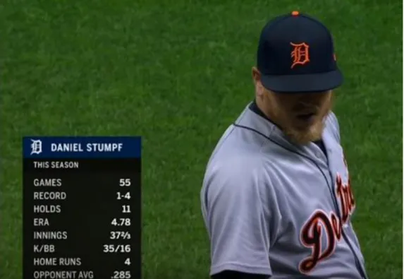
To see how well-integrated statistics are, one only needs to watch a game for five minutes. As soon as a batter walks up to plate, his season statistics show up in on the screen. From how well the player has gotten on base to how many home runs he has scored, the watcher instantly gets an idea of the player's caliber. The same happens with the pitcher who has his pitching stats displayed frequently during the game (Figure 2).

*

(13)

7

Basic statistics are mixed-in with more advanced ones build with algorithms. These sta-tistics are not only used to benefit the fans, but also the team itself. Major League teams have data analysis departments whose output is taken into serious consideration as the general manager makes his decisions. An example of a team build solely on statistics is given in Chapter 3.4. (8; 9)

3.3 Sabermetrics

Sabermetrics was created by The Society for America Baseball Research to better measure players' in-game performance. Core skills of sabermetrics are to ask the correct question and to use statistics correctly. Math is not required but logical reasoning is im-portant. They use traditional statistics like Batting Average and Earned Run Average to create more advanced metrics like the On-base percentage.

𝑂𝑛 𝑏𝑎𝑠𝑒 𝑝𝑒𝑟𝑐𝑒𝑛𝑡𝑎𝑔𝑒 = 𝐻𝑖𝑡𝑠+𝐵𝑎𝑠𝑒 𝑜𝑛 𝐵𝑎𝑙𝑙+𝐻𝑖𝑡 𝑏𝑦 𝑃𝑖𝑡𝑐ℎ

𝐴𝑡 𝑏𝑎𝑡𝑠+𝐵𝑎𝑠𝑒 𝑜𝑛 𝐵𝑎𝑙𝑙+𝐻𝑖𝑡 𝑏𝑦 𝑃𝑖𝑡𝑐ℎ+𝑆𝑎𝑐𝑟𝑖𝑓𝑖𝑐𝑒 𝐹𝑙𝑖𝑒𝑠 (1)

• At bats are the number of turns the player has against the pitcher

• Hits are number of times the player has gotten into a base by hitting the ball

• Base on ball means the number of times the player has gotten on base by the pitcher throwing four balls. Ball means that he pitched out of the strike zone four times.

• Hit by Pitch is when the batter gets hit by the pitcher’s throw. That gives the batter a free walk to the first base.

• Sacrifice fly happens when there is a runner in the bases, and the batter hits the ball so that the runner is able to score, but the batters play results in an out. For example, the batting team has one out so far and a runner on the second base. A batter comes in and hits the ball far out to the outfield where a defender catches it. After the defender caught the ball, the runner on sec-ond can start to run to third base and eventually home base. If the runner gets to the home plate before the ball does, the result of the play is a sacrifice fly

(14)

8

meaning that a run was scored, and an out was given. Sacrifice flies are only possible when the batting team has one or fewer outs in an inning because the out count goes to three before the runner can score.

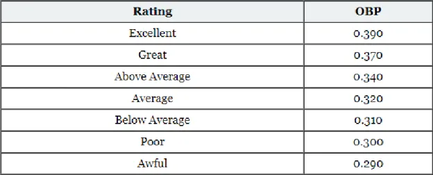
The algorithm shown in Figure 3 is just one version on how to calculate the on-base percentage.

Figure 3. Suggested ratings for the algorithms results.

Sabermetrics has professional data analysts and a devoted community who are always trying to improve the algorithms used. (12; 13; 14)

3.4 Moneyball

What would happen if a team was built only on sabermetrics? That was the revolutionary plan of the general manager of the 2002 Oakland Athletics MLB team, Billy Beane. In a league that boasted such worldwide known teams as the New York Yankees and the Los Angeles Dodgers, the Athletics budget could not hold a candle against them. As bigger teams got all the star players, Beane had to come up with something different to compete in the league. The plan was to look for non-star players that other teams did not value but who had good sabermetric statistics. Sabermetrics usage in professional baseball was in its early days in 2002, so it did not play a significant role usually in team’s player decisions.

(15)

9

Instead of concentrating on individual statistics such as home runs, more weight was given statistics closely linked with winning games. Beane focused on getting players that would specifically help the team in the statistical areas that were found to be the most critical factors in the team’s success. These factors were calculated with specialized mathematics. For batters, instead of the traditional measures of a player’s ability, batting average, home runs and runs batted in, more advanced statistics were used. These were on-base percentage that was detailed before and slugging percentage, which is an al-gorithm measuring the batting productivity of the batter. (15)

So how did the 2002 Oakland Athletics fare with their sabermetrics tactics in the ex-tremely competitive league? Against the odds, they made the playoffs without having the star players of the bigger teams. In the next year, Billy Beane and his innovative strategy were made famous by Michael Lewis’s book titled Moneyball. The book, along with a movie, has made sabermetrics popular not only with baseball but in other sports as well. These days all the other MLB teams have also embraced sabermetrics as a part of team building. (16)

4 Machine Learning

Machine learning is a branch of artificial intelligence based on the concept of a computer studying their experience and then making predictions based on the knowledge gained without too much human interference. It enables computers to make data-driven deci-sions rather than needing the developer to program the computer to do specific tasks. Algorithms used in machine learning utilize statistics to find patterns and apply them in significant amounts of data. The training data set is used to train the algorithm to build a model. When the algorithm is introduced new data, a prediction is created based on the model. Training commences until the accuracy of the prediction is evaluated to be good enough, and then the algorithm is deployed. Machine learning can be found everywhere these days, from Netflix’s suggestions on what to watch next to self-driving cars. Fur-thermore, its usage is only growing. (17; 18)

There are multiple ways to approach machine learning. Two different learning algorithms, Supervised and unsupervised learning, are introduced here. Also, three techniques, classifiers, linear regression, and clustering, are discussed. The latter utilizes

(16)

10

unsupervised learning, while the first two use supervised learning. Further details are given on two classification algorithms, decision tree, and neural network.

4.1 Supervised and Unsupervised Learning

Supervised and unsupervised learning are two main fields in machine learning. Super-vised learning can be grouped into classification and regression. Clustering and associ-ation are sub-groups of unsupervised machine learning. In practical machine learning, supervised learning is used by the majority.

With supervised learning, the model is trained with data that is labeled with the correct answers until the algorithm achieves an acceptable level of accuracy. After the training, the model is given a new set of data, and it will generate an output. The purpose of this learning type is to learn a function that best app estimates the relationship between input and output data when it is given a set of data and desired outputs.

With unsupervised learning, there are no output variables; instead, there is only input data. This means that there is not a guaranteed way to compare model performance in most of these sorts of learning types. The algorithm discovers and uses structures hidden in the data on its own. Patterns, similarities, and differences are used to group unsorted information. (19; 20; 21)

4.2 Classifiers

With classification techniques, applications can predict distinct responses; for example, which team is going to win a baseball game. This is achieved by approximating a map-ping function (f) from input variables (x) to discrete output variables (y). Input variables in the baseball example could be how well the team hits the ball with teams batting av-erage percentage and how well they do they pitch to the opposition with pitching avav-erage percentage. Output variables, in this case, are a win or a loss as there are no draws in baseball, making it a binary classification. More classes can be added if needed by the model.

(17)

11

For example, a football game has three possible results, so three classes are needed. First, feed the classifier with some training data of past matches so it can understand how given input variables relate to the class. Then it can be used to predict matches yet to played. The accuracy prediction depends on how good the classifier training was and the amount of the training data. (22)

4.2.1 Decision Tree

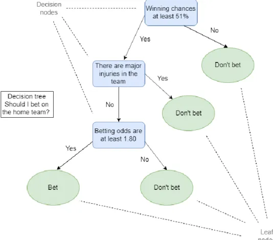
The decision tree is one of the more simpler classification algorithms. The name comes from the fact that the model forms a tree-like structure, having the root node alone at the top and then every row widening with decision nodes and leaf nodes. This is shown in Figure 4.

Figure 4. Decision tree based on betting on baseball.

The recursive divide-and-conquer method is used to construct the tree from the top downwards. Meaning that the problem is broken down to smaller problems over and over

(18)

12

until it is simple enough to be solved. Training data is used in sequence, and afterward, a rule is learned. Every time a rule is learned, the sequence covered by the rules is removed. A developer has to be careful not to give the tree too many branches leading to a poor performance on the data desired to predict. (23)

4.2.2 Neural Network

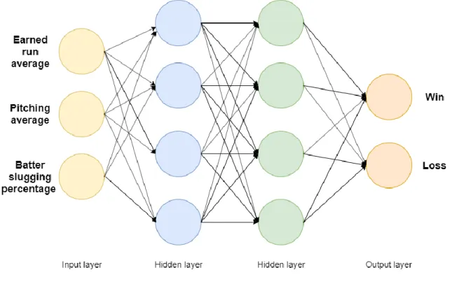
A neural network is a series of algorithms, based loosely on the human brain, designed to recognize patterns. The network consists of an input layer, output layer, and any num-ber of hidden layers (Figure 5). These layers contain nodes, which is the place where the computation happens. Each connection a node has a weight associated with it. When one weight is changed, it affects all the nodes, as well. By adjusting these weights during the learning phase, the network can create a prediction. At the start the model knows nothing about the weights and starts with a guess. It will improve the guesses by learning from mistakes during the training.

Figure 5. Neural network for predicting the result of a baseball game.

A hidden layer between input and output is essentially a stack of models where each node acts as a model. It gets its name from the fact that the nodes in the layer have no

(19)

13

direct connection with the outside world and instead communicate with input and output nodes. Hidden layers enable the modeling of complex relationships. The more there are hidden layers, the more complex the network gets, but it also takes more time the model takes to train and adjust weights. (24; 25; 26)

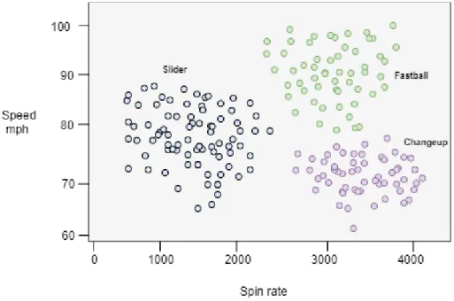
4.3 Clustering

Clustering is one of the most popular unsupervised classification techniques. The tech-nique aims to divide the points of data into smaller groups by the similarity of their traits as seen in Figure 6. For example, one can organize movies according to the genre or topic.

Figure 6. Clustering with different styles of baseball pitches. The numbers are only examples.

Clustering can be divided into two groups; hard clustering means that a data point can only either belong to the cluster or not belong. With soft clustering, a data point is given a probability of it belonging to the given clusters.

One of the most used clustering algorithms is K-means. It is a simple algorithm that di-vides the data points into clusters according to which is their nearest mean, serving as a prototype of the cluster. The results can vary if the algorithm is run multiple times, as the

(20)

14

algorithm starts up with a random number of clusters. K-means algorithm works well with big data.

Another popular algorithm is hierarchical clustering. The algorithm starts with all the data points in their clusters. Then it will build a hierarchy of clusters until there are only two left. The last two will merge into one, and the algorithm is complete. Unlike K-means, hierarchical clustering does not work well with big data.

Clustering is used, for example, with recommendation engines, medical imaging, and grouping of search results. (27; 28)

4.4 Linear Regression

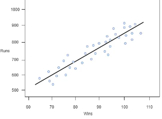
Linear regression is one of the most well-known algorithms and an excellent place to start with machine learning. It is one of the more accessible algorithms to start, and no background in statistics or algebra is needed. As seen in Figure 7, the simpleness of the model representation is one of the linear regressions draws.

(21)

15

Linear regression is used to model the relationship between a target variable and at least one predictor variable. It is done by fitting a linear equation to the data that has been examined. This straight line is also known as the regression line. There are two different kinds of linear regression, simple and multiple. As the names indicate, the difference is between these two types is the number of predictor variables, single having one variable and multiple linear regression having more than one variable. (29)

5 Library Comparisons

JavaScript has a good offering of machine learning libraries. Researching for this thesis, libraries for various scenarios with different strengths were found. This chapter, briefly goes through four of them and explains the reasons for choosing the library for the ap-plication.

5.1 Tensorflow.js

TensorFlow.js is an open-source JavaScript library for machine learning to be used either in the browser or Node.js. This library was pre-dated by the main TensorFlow library used popularly with Python. Tensorflow.js brings all the core features like defining, train-ing, and running machine learning models to be used together with JavaScript client-side scripting, bringing more interactive elements to machine learning. Models made in Ten-sorFlow can be converted to TenTen-sorFlow.js and then be loaded into the browser or re-trained. (30; 31)

5.2 Brain.js

Brain.js is an open-source library of neural networks written JavaScript. It is meant to be used with Node.js and browsers and advertises itself as simple and easy to use. It aims to achieve this by lessening the importance of math and making sure the need to use APIs is limited. Because of this, the customizable options are not as numerable as some other libraries. The author of the brain.js, Robert Plummer, provides a thorough tutorial and is heavily involved in the continued development of the library. (32; 33)

(22)

16

5.3 Synaptic

Synaptic is another neural network library written in JavaScript for node.js and the browser. It differentiates itself as being architecture-free, so there is freedom for devel-opers to choose what kind of neural network architecture they want to build. However, if ready-made architecture is needed, those too can be found as Synaptic has a few built-in architectures. The creator offers multiple demos and to see how Synaptic works and further documentation on neural networks themselves. (34)

5.4 ConvNetJS

Initially written by Tesla’s director of AI Andrej Karpathy when he was a Ph.D. student at Stanford, ConvNetJS is a JavaScript library for neural networks. Making it unique in the space is that it is used entirely in a browser. There is no need to install anything or to have a powerful computer to run the training of the model. There are several browser demos on the project’s homepage. The library has been expanded since its creation by community members and is open for more improvements. (35)

5.5 Library for Application

For this project, TensorFlow.js with Node.js was the best option Node.js had been used before, and it also made it possible to use the Heroku platform to host the application. Another factor was that TensorFlow.js is the most popular JavaScript library for machine learning, making it was easier to find tutorials and information about it. The library was found to be easily accessible and well documented. The author had a little experience with machine learning with Python, and the syntax was similar to TensorFlow.js, so it was easier to start with than other libraries.

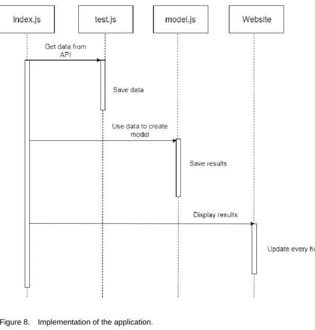
6 Implementation

(23)

17

Figure 8. Implementation of the application.

The product of the application can be seen on the website that the application produces. It displays the game information with prediction of the model as seen in Figure 9.

(24)

18

If the game has not yet been played, the starting time of the game is shown instead of the final score. If the game is ongoing, the current score is displayed.

6.1 Test Data

The data that is used to train the model is from the MySportsFeed feed called Seasonal Team Stats. It gives over one hundred statistics of each team on a given day. If no date is given, it defaults to the current date.

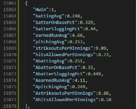
At first, an application called Postman had to be used to get the data and then manually copy and paste the data points to the test data JSON-file as seen in Figure 10. After having copied the statistics, the winner of the match was looked up at the MLB’s official website and the “Hwin” data point was written. Zero meant that the away team won, and one meant that the home won. This manual adding of the data took some time, but some data was needed to start working on the model.

Figure 10. A singular entry on the test data JSON-file.

Later on, a feature that fetches the data on a specific day and takes the data points automatically was created. Then the winning percentages are added for each match, and it is saved as JSON-file. Now it was only necessary to add the “Hwin” data point got

(25)

19

from the scoreboard in the application webpage. This sped up the data collecting im-mensely.

In the later parts of the project, it was noticed that a mistake had been made when calling the data feed. For the date parameter name, “fordate” had been used which was the same when calling the scoreboard feed. This was incorrect, as with this feed, the param-eter name had to be “date”. It made it so that the date always defaulted to the current date, giving me incorrect days statistics. After noticing this, it was realized that the whole test data had to be redone, which was then carried out.

6.2 Model Used in Application

From the over 100 statistics given in the API feed, the most important ones for the appli-cation had to be chosen. This was done using the author’s experience with following the sport. This is because some of the statistics are irrelevant to the objectives of the project and giving too many data points would create a model that focused on the wrong things. Data points that were percentages were chosen, as choosing a statistic such as the number of hits was always growing throughout the season and made no sense to be included in the model.

In the model, six data points for each team were used. The points were

• Batter on base percentage which tells how well the team's hitters get on base. There are a few ways of getting on base in baseball and this data points gath-ers all of them in one algorithm.

• Batter slugging percentage which tells how well the team's hitters hit when other player or players are in scoring position. It is useless to get on base if there are no batters to advance the player to the home plate to score points. In sports terms, this is known as "clutch," as in the ability to perform in situa-tions where it is most needed under pressure.

• Earned run average which tells how many runs the team scores on average in a game. Gives the big picture of the team’s offence.

(26)

20

• Pitching average which tells how many runs the team gives up on average in a game. Statistic demonstrates the team’s defense abilities as a whole.

• Strikeouts per 9 innings which tells how many strikeouts on average the team gets in a game. It is essential to get information about the team’s pitchers capability to end the opposition batters turn cleanly.

• Hits allowed per 9 innings which tells how many hits the team allows on av-erage in a game. Giving hits allows the opposition scoring changes and ex-tends the inning for further possible hits. Gives glimpse to the team’s pitchers abilities to keep opposition off the bases.

In the beginning, the model also contained Batting average, which tells how well the team's hitters hit the ball into play. It is still in the test data, but it is not included in the mapping of the model. The decision was made because the model already used more complex statistics to calculate batting prowess making the simple algorithm batting average redundant.

6.3 Frontend

One HTML-page and one CSS were used in the application. The HTML-page contains a small amount of JavaScript code. JsRender and jQuery libraries are utilized in display-ing the scoreboard. The scoreboard that is displayed on the website gets its information from a JSON file that has the day's games with all of the home teams winning percent-ages added to it.

CSS has a small amount of code to create a simple look for the site as the frontend was not a focus in the project. In addition to the teams playing, the starting time and the home winning percentage is shown. If the game is ongoing or has ended, the score is also displayed.

(27)

21

6.4 Backend

Node.js runtime was used to create the backend with the help of a web application frame-work called Express. The application can be deployed to the local environment or the Heroku platform. The index page collects all the JavaScript pages and asynchronous calls them. On the page the application is divided into three parts: Getting the data, cre-ating a model (Listing 1), and lastly, showing it all on the website.

const modelCreating = async () => { var model = require('./static/model')

await model.createModel().then((result) => { newestData = result;

}); }

modelCreating();

Listing 1. Creating the model in the index.js

There is also a function that sets up how often the scoreboard gets updated with new data. The API gives new data every ten minutes, but because real-time scores are not important in the scope of this project, the updating interval is set to one hour. The interval can easily be changed if the need arises.

6.4.1 Getting the Data

The API is called twice, first for the day's scoreboard as seen in Listing 2 and secondly for every team's stats as of today.

exports.getData = async function () {

return msf.getData('mlb', '2019-regular', 'scoreboard', 'json', { fordate: today.getFullYear() + ('0' + parseInt(today.getMonth())).slice(-2) + ('0' + today.getDate()).slice(-2), force: true }) }

Listing 2. Calling the API for todays scoreboard data.

After, the JSON file with the team statistics is worked on by page called dataSetup.js. It setups a JSON file with only the teams playing today with only the statistics used in the model later.

(28)

22

6.4.2 Managing Data

As the statistics feed provides a JSON with all teams and their statistics, a modification is needed. Listing 3 shows the dataSetup.js that doing just that.

var gameStatsJson = [];

var teams = [];

exports.getTodaysJsonData = async function () {

teamStatsString = "seasonal_team_stats-mlb-2019-regular-" + fordate + ".json"

scoreboardInformation = "scoreboard-mlb-2019-regular-" + fordate + ".json" var teamStatsObject = require('../results/' + teamStatsString);

var teamsPlaying = require('../results/' + scoreboardInformation); var temp = Object.values(teamStatsObject);

var arrayOfTeamStats = temp[1];

var teamsPlayingTemp = Object.values(teamsPlaying); var tempteams = Object.values(arrayOfTeamStats)

var arrayOfTeamsPlaying = teamsPlayingTemp[0].gameScore; // create data for all the teams

arrayOfTeamStats.forEach(team => { var teamStats = {}; teamStats["ID"] = team.team.id; teamStats["battingAvg"] = team.stats.batting.battingAvg; teamStats["batterOnBasePct"] = team.stats.batting.batterOnBasePct; teamStats["batterSluggingPct"] = team.stats.batting.batterSluggingPct; teamStats["earnedRunAvg"] = team.stats.pitching.earnedRunAvg; teamStats["pitchingAvg"] = team.stats.pitching.pitchingAvg; teamStats["strikeoutsPer9Innings"] = team.stats.pitching.strikeoutsPer9In-nings; teamStats["hitsAllowedPer9Innings"] = team.stats.pitching.hitsAl-lowedPer9Innings; teams.push(teamStats); }) arrayOfTeamsPlaying.forEach(game => {

for (var i = 0; i <= teams.length - 1; i++) { if (teams[i].ID == game.game.homeTeam.ID) { var homeTeam = teams[i];

}

if (teams[i].ID == game.game.awayTeam.ID) { var awayTeam = teams[i];

} }

//Create json for todays team var tempMatch = { battingAvg: homeTeam.battingAvg, batterOnBasePct: homeTeam.batterOnBasePct, batterSluggingPct: homeTeam.batterSluggingPct, earnedRunAvg: homeTeam.earnedRunAvg, pitchingAvg: homeTeam.pitchingAvg, strikeoutsPer9Innings: homeTeam.strikeoutsPer9Innings, hitsAllowedPer9Innings: homeTeam.hitsAllowedPer9Innings,

(29)

23 AbattingAvg: awayTeam.battingAvg, AbatterOnBasePct: awayTeam.batterOnBasePct, AbatterSluggingPct: awayTeam.batterSluggingPct, AearnedRunAvg: awayTeam.earnedRunAvg, ApitchingAvg: awayTeam.pitchingAvg, AstrikeoutsPer9Innings: awayTeam.strikeoutsPer9Innings, AhitsAllowedPer9Innings: awayTeam.hitsAllowedPer9Innings } gameStatsJson.push(tempMatch) }) fs.writeFileSync('daysGameData.json', JSON.stringify(gameStatsJson),) }

Listing 3. Creating day specific JSON files of the scoreboard and team statistics.

The JSON of the feed is taken and put to a variable called “arrayOfTeamStats.” The statistics used in the model are then picked up from the JSON and pushed to an array called “teams,” each team and their statistics as induvial variables.

As the array now includes all the thirty teams of the MLB, there is a need to cut down on the amount to have only the teams playing today. This is done by checking the team’s id against the scoreboard JSON as they use the same ids for the teams. If the id exists, then the team is playing today. The teams are also divided into home and away teams at this point.

Creating the final look of JSON that is used by the model is next. The home and away teams seven data points are put into an array as variables. This array is then stringified to JSON format, and finally, the new file is written called “daysGameData.json.” This is the JSON file that the model uses when predicting the day’s games.

6.4.3 Creating the Model

Next, the model for the prediction was created. It takes the JSON file created in the data setup and maps it into a 2D tensor. Also, the training data that was created before is mapped to a 2D tensor (Listing 4).

const testingData = tf.tensor2d(daysGameData.map(match => [match.battingAvg, match.batterOnBasePct, match.batterSluggingPct, match.earnedRunAvg,

match.pitchingAvg, match.strikeoutsPer9Innings, match.hitsAllowedPer9Innings, match.AbattingAvg, match.AbatterOnBasePct, match.AbatterSluggingPct,

(30)

24

match.AearnedRunAvg, match.ApitchingAvg, match.AstrikeoutsPer9Innings, match.AhitsAllowedPer9Innings]), [daysGameData.length, 14])

Listing 4. Mapping the testing data.

The model is told that a game has two possible results win or a loss, represented by a one and a zero (Listing 5).

const outputData = tf.tensor2d(testdata.map(match => [ match.Hwin === 'W' ? 1 : 0,

match.Hwin === 'L' ? 1 : 0, ]), [1244, 2])

Listing 5. Creating the model

The model calculates the probability of the home team's win with the help of several layers. For compiling, the categorical Cross-entropy function is used for loss. Categorical Cross-entropy is a loss function meant for single label classification models. Single label means that only one result can correct. When the function's value goes down, it means that the prediction gets more accurate. When the value is zero, it means the prediction is at its best, and the model is well trained. (36)

For the optimizer, the Adam algorithm is used. The name comes from the word’s adap-tive moment estimation. It is one of most popular optimizing algorithms used in deep learning because of its simplicity and efficiency. The training uses forty epochs for forty times.

After the prediction is finished, the home teams winning percentage is added to a JSON file with the scoreboard information as another item in the game array. This is the JSON file used in the frontend.

6.4.4 Building Website

Lastly, the website was put together to be viewable on the localhost or the Heroku plat-form as seen in Listing 6.

const website = async () => { app.set('view engine', 'ejs');

app.engine('html', require('ejs').renderFile); await app.get('/', function (req, res) {

(31)

25

res.sendFile(__dirname + '/index.html', {test:test.toString()}); });

app.use('/static', express.static(__dirname + '/static')); app.use(express.static(__dirname));

http.listen( process.env.PORT || 4400, function () { console.log('HTTP server started on port 4400'); });

io.on('connection', function (socket) { socket.emit('data', newestData); });

}

website();

Listing 6. Creating the website in index.js. “process.env.PORT” is the port for Heroku.

All this is executed by using the command node index.js in the command line or an equivalent application.

7 Results and Future Considerations

This chapter explains model overfitting and how to prevent it. The testing phase is de-scribed from the plan to the actual testing and finally the chapter introduces the results and possible improvements.

7.1 Model Overfitting

In the creation of the model’s prediction, there is a balancing act of having the model be too simple or too complicated. Having the model fit the data is a crucial concept in ma-chine learning and important to understand to be able to create efficient models.

Model overfitting means that the model tries too hard to account for all possible trends or structures on the training data. It is a common problem in machine learning. Overfitting can happen when there are too many parameters for the model to consider. The model cannot find the true underlying pattern and instead focuses on insignificant information and randomness. It fits well with the training data but is not a good fit with new sets of data. This can be avoided by simplifying the model. To decrease the complexity, de-creasing the number of layers, and the nodes that are in them is a good idea.

(32)

26

One way of detecting overfitting models is to look at the accuracy number. It is a red flag if the model does significantly better with the training data than with the testing set. (37)

7.1.1 Model Underfitting

Model underfitting is the opposite problem of overfitting that can also occur if the model is too simple. This means that the model is either regularized too much or takes into consideration too few aspects. Underfitting models produce predictions with less devia-tion in their predicdevia-tion but more bias towards wrong results. (37)

7.1.2 Prevention

To prevent overfitting, one should start by creating a benchmark model. The model should be simple by not having many nodes or layers. This benchmark can be then ref-erenced to see how added complexity affects the fitting.

Another good idea is to add more training data if possible. This can improve the model’s ability to recognize the true patterns. As always, with machine learning, the data should be clean and relevant to the issue that is being predicted.

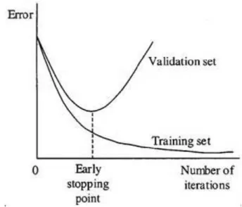
As seen in Figure 11, a technique called early stopping can help prevent overfitting. The iterations of how many times the model goes through data, help model improve. If done too many times, however, the model will start to overfit training data. Early fitting means stopping the iterations before this overfitting starts happening.

(33)

27

Figure 11. Early stopping technique.

The last two techniques are regularization and ensembling. Regularization means one artificially makes the model simpler by utilizing a varying range of techniques. Depending on the learner in use, different methods are available. With ensembling, one combines from multiple different models. As with regularization, there are various methods availa-ble to improve the model. (37)

7.2 Testing Plan

The first idea on how to test the prediction quality of the application was to get a data set from one MLB season and then test it on a different season, but this turned out to be impossible. The testing scope is limited by the fact that MySportsFeed API only provides the statistical data needed for the 2019 season. This is because this specific feed is a recent one that was only implemented before the latest season.

Now the testing was done by getting the data feed from the 25th of June onwards, giving the learning data 1244 games to learn from. This leaves another # games for testing. The earlier games are ignored as the statistics of each team need time to balance out and do not give a good representation of the team.

The testing process was simple, the date was manually changed, and the winning per-centage, along with the final score, was displayed on the application. Whichever team

(34)

28

the application predicted to win, won, it got a correct mark. Otherwise, an incorrect marked and in the case where it predicts the odds to be even, no marks were given.

7.3 Testing

Before testing, an accuracy metric was added to the training function. The results re-vealed that the model was overfitting. As no more training data could be added due to the lack of it, it was necessary to start with a benchmark model and move forward from there.

The testing was done manually by changing the date and running the application. A function was used to load the model to make the process faster. The results from the website were marked into Excel which was used to calculate the percentages for the models and also to compare them.

7.3.1 Creating Benchmark Model

To create a benchmark model, only two data points for each team were selected for the model. This was easily done as the eight other points were simply removed and the length changed, as seen in Listing 7.

const trainingData = tf.tensor2d(testdata.map(match => [

match.earnedRunAvg, match.pitchingAvg, match.AearnedRunAvg, match.Apitch-ingAvg

]), [ 1244, 4])

const testingData = tf.tensor2d(daysGameData.map(match => [

match.earnedRunAvg, match.pitchingAvg, match.AearnedRunAvg, match.Apitch-ingAvg

]), [daysGameData.length, 4])

Listing 7. Mapping the benchmark model.

The data points on the benchmark model are earned run average to have an idea of the offenses prowess and pitching average to a sense of the defense. Running through the training with this model produced great results and accuracy.

(35)

29

7.3.2 Modifying Original Model

It was decided to experiment with the old model and see if the fit could be made better. After testing various setups, it was found difficult to get a good fit with the training data available. So, the decision was made to trim the data point number in order to avoid overfitting. The model ended up with six data points: batter slugging percentage, earned run average and pitching average for both of the teams. With these data points, it was possible to get the model fit well with reasonable accuracy.

7.3.3 Test Results

Both the benchmark model were tested and the modified original model were tested as illustrated in Figure 12. The benchmark scored 50% and the modified original model scored 62% predictions correct. This is a good result for the modified model and a good platform for which to build on.

Figure 12. Test results from the start and the end of the test.

One inspection note was that there were a lot of 50/50 of winning percentages. This makes sense because MLB is a very even league. The simple model preferred home teams more while the modified original model was more even with the home versus away split.

(36)

30

7.4 Future Improvements

The model will improve noticeably with more training data. The aim is to add this when the next season of Major League Baseball starts up again in March as it is currently in the off-season. With more data, all the data points planned but not included in the model can be utilized. After the additional data is added, one can compare the models and see the improvement.

There is also a possibility to experiment with different data points and setups to see how the predictions are affected. Also, using different algorithms could be an excellent testing and learning opportunity.

There is also interest in expanding into other sports by creating another model similar to this one. A few options would be ice hockey and football. These sports have also em-braced statistics as a part of the sports. For example, the National Hockey League, the top ice hockey league, has a similar statistics feed like the ones used in this project from MySportsFeed. Ice hockey has also accumulated a following of people creating their sabermetrics. One of the most popular of these statistics is called Corsi, which is an advanced statistic looking at the shot differential in even-strength situations. As this ex-ample shows, ice hockey has excellent potential for a similar model. (38)

8 Conclusions

In this bachelor’s thesis, the goal was to investigate the suitability of JavaScript to be used with machine learning, compare JavaScript’s machine learning libraries, and de-velop an application that uses one of these libraries. All of these goals were achieved during the making of the project. There were problems along the way as there are in all projects, and they served as valuable learning moments.

The major part of the time was spent on the application. Building it from the ground up and learning firsthand. The thesis gives insight into machine learning and how to imple-ment it with JavaScript for anyone interested in these subjects and gives a good starting off point into learning more.

(37)

31

The model created during this process has great potential to be experimented with and improved. Similar models can be created for other sports as well. The original model was not perfect, but it gave a good baseline on which to improve and gave much valuable information to learn more about what makes an effective model. How to improve the fitting of the model was also documented and taken into use.

In the theory part, it is explained how even though JavaScript is not widely considered as a language for machine learning is a worthy language to consider when starting a project. Libraries introduced have their strengths, which need to be taken into consider-ation when choosing a library for an applicconsider-ation.

References

1. Tutorialspoint. [Online] 2019. [Cited: Oct 13, 2019.] https://www.tutorialspoint.com/javascript/javascript_overview.htm.

2. IT Pro Today. [Online] 2012. [Cited: Nov 24, 2019.] https://www.itprotoday.com/web-application-management/meet-jsrender-next-version-jquery-templates.

3. Ornbo, George.Sams Teach Yourself Node.js in 24 Hours: Sams Teac Your node 24 hour. 2013. pp. 6-8.

4. Node.js. [Online] 2019. [Cited: Oct 13, 2019.] https://nodejs.org/en/about/.

5. Git. [Online] 2019. [Cited: Oct 14, 2019.] https://git-scm.com/book/en/v1/Getting-Started-Git-Basics.

6. Atlassian. [Online] 2019. [Cited: Oct 14, 2019.] https://www.atlassian.com/git/tutorials/what-is-git.

7. ESPN Front Row. [Online] 2011. [Cited: Oct 10, 2019.] https://www.espnfrontrow.com/2011/07/happy-10th-birthday-k-zone/.

8. Beyond the Boxscore. [Online] 2014. [Cited: Oct 10, 2019.]

(38)

32

9. Taylor & Francis Online. [Online] 2017. [Cited: Oct 10, 2019.] https://www.tandfonline.com/doi/full/10.1080/10691898.2002.11910663.

10. Fangraphs. [Online] 2019. [Cited: Oct 10, 20119.] https://tht.fangraphs.com/brewers-tv-statistician-mike-falkner-and-the-evolution-of-baseball-broadcasts/.

11. —. [Online] 2010. [Cited: Oct 10, 2019.] https://library.fangraphs.com/offense/obp/. 12. Costa, Gabriel B, Huber, Michael R and Saccoman, John T. Practicing Sabermetrics: Putting the Science of Baseball Statistics to Work. 2009. pp. 6-12.

13. Sean Lahman. [Online] 2019. [Cited: Oct 12, 2019.] http://www.seanlahman.com/baseball-archive/sabermetrics/sabermetric-manifesto/. 14. SABR. [Online] 2019. [Cited: Oct 12, 2019.] https://sabr.org/sabermetrics/the-basics. 15. The Sport Journal. [Online] 2018. [Cited: Oct 12, 2019.] https://thesportjournal.org/article/general-managers-and-the-importance-of-using-analytics/.

16. SFGate. [Online] 2011. [Cited: Oct 12, 2019.]

https://www.sfgate.com/athletics/article/Michael-Lewis-on-A-s-Moneyball-legacy-2309126.php.

17. SAS. [Online] 2019. [Cited: Sep 10, 2019.]

https://www.sas.com/en_us/insights/analytics/machine-learning.html.

18. Edureka. [Online] 2019. [Cited: Sep 10, 2019.] https://www.edureka.co/blog/what-is-machine-learning/#ML.

19. Geeks for Geeks. [Online] 2019. [Cited: Oct 16, 2019.] https://www.geeksforgeeks.org/supervised-unsupervised-learning/.

20. Towards Data Science. [Online] 2018. [Cited: Oct 16, 2019.] https://towardsdatascience.com/supervised-vs-unsupervised-learning-14f68e32ea8d. 21. Machine Learning Mastery. [Online] 2019. [Cited: Oct 16, 2019.] https://machinelearningmastery.com/supervised-and-unsupervised-machine-learning-algorithms/.

22. Towards Data Science. [Online] 2018. [Cited: Oct 7, 2019.] https://towardsdatascience.com/machine-learning-classifiers-a5cc4e1b0623.

23. —. [Online] 2018. [Cited: Oct 7, 2019.] https://towardsdatascience.com/machine-learning-classifiers-a5cc4e1b0623.

24. —. [Online] 2019. [Cited: Oct 7, 2019.]

https://towardsdatascience.com/understanding-neural-networks-19020b758230.

(39)

33

26. Ujjwal, Karn. [Online] 2016. [Cited: Oct 7, 2019.] https://ujjwalkarn.me/2016/08/09/quick-intro-neural-networks/.

27. Geeks for Geeks. [Online] 2019. [Cited: Oct 16, 2019.] https://www.geeksforgeeks.org/clustering-in-machine-learning/.

28. Analytics Vidhya. [Online] 2016. [Cited: Oct 16, 2019.]

https://www.analyticsvidhya.com/blog/2016/11/an-introduction-to-clustering-and-different-methods-of-clustering/.

29. Machine Learning Mastery. [Online] 2019. [Cited: Nov 17, 2019.] https://machinelearningmastery.com/linear-regression-for-machine-learning/.

30. Medium. [Online] 2018. [Cited: Sep 25, 2019.]

https://medium.com/tensorflow/introducing-tensorflow-js-machine-learning-in-javascript-bf3eab376db.

31. Tensorflow. [Online] 2019. [Cited: Sep 25, 2019.] https://www.tensorflow.org/js. 32. Brain.js. [Online] 2019. [Cited: Sep 27, 2019.] https://brain.js.org.

33. Stack Abuse. [Online] 2019. [Cited: 27 Sep 2019.] https://stackabuse.com/neural-networks-in-javascript-with-brain-js/.

34. Github. [Online] 2019. [Cited: Sep 28, 2019.] https://github.com/cazala/synaptic. 35. Stanford University. [Online] 2019. [Cited: Sep 28, 2019.] https://cs.stanford.edu/people/karpathy/convnetjs/.

36. Peltarion. [Online] 2019. [Cited: Nov 9, 2019.] https://peltarion.com/knowledge- center/documentation/modeling-view/build-an-ai-model/loss-functions/categorical-crossentropy.

37. Elite Data Science. [Online] 2019. [Cited: Nov 10, 2019.] https://elitedatascience.com/overfitting-in-machine-learning.

38. Calgary Herald. [Online] 2014. [Cited: Nov 24, 2019.] http://www.calgaryherald.com/Sports/Wilson+know+Corsi+Here+handy+dandy+primer +advanced+stats/10265096/story.html.

39. MySportsFeeds. [Online] 2019. [Cited: Nov 5, 2019.] https://www.mysportsfeeds.com/.

40. Google. [Online] 2019. [Cited: Oct 16, 2019.] https://developers.google.com/machine-learning/clustering/overview.