Zurich Open Repository and Archive University of Zurich Main Library Strickhofstrasse 39 CH-8057 Zurich www.zora.uzh.ch Year: 2018
Hydrological modeling to evaluate climate model simulations and their bias
correction
Hakala, Kirsti ; Addor, Nans ; Seibert, Jan
Abstract: Variables simulated by climate models are usually evaluated independently. Yet, climate change impacts often stem from the combined effect of these variables, making the evaluation of inter-variable relationships essential. These relationships can be evaluated in a statistical framework (e.g., using correlation coefficients), but this does not test whether complex processes driven by nonlinear re-lationships are correctly represented. To overcome this limitation, we propose to evaluate climate model simulations in a more process-oriented framework using hydrological modeling. Our modeling chain consists of 12 regional climate models (RCMs) from the Coordinated Downscaling Experiment–European Domain (EURO-CORDEX) forced by five general circulation models (GCMs), eight Swiss catchments, 10 optimized parameter sets for the hydrological model Hydrologiska Byråns Vattenbalansavdelning (HBV), and one bias correction method [quantile mapping (QM)]. We used seven discharge metrics to explore the representation of different hydrological processes under current climate. Specific combinations of biases in GCM–RCM simulations can lead to significant biases in simulated discharge (e.g., excessive precipitation in the winter months combined with a cold temperature bias). Other biases, such as exaggerated snow ac-cumulation, do not necessarily impact temperature over the historical period to the point where discharge is affected. Our results confirm the importance of bias correction; when all catchments, GCM–RCMs, and discharge metrics were considered, QM improved discharge simulations in the vast majority of all cases. Additionally, we present a ranking of climate models according to their hydrological performance. Ranking GCM–RCMs is most meaningful prior to bias correction since QM reduces differences between GCM–RCM-driven hydrological simulations. Overall, this work introduces a multivariate assessment method of GCM–RCMs, which enables a more process-oriented evaluation of their simulations.
DOI: https://doi.org/10.1175/JHM-D-17-0189.1
Posted at the Zurich Open Repository and Archive, University of Zurich ZORA URL: https://doi.org/10.5167/uzh-152148
Journal Article Published Version Originally published at:
Hakala, Kirsti; Addor, Nans; Seibert, Jan (2018). Hydrological modeling to evaluate climate model simulations and their bias correction. Journal of Hydrometeorology:1321-1337.
NANSADDOR
Department of Geography, University of Zurich, Zurich, Switzerland, and Research Applications Laboratory, National Center for Atmospheric Research, Boulder, Colorado, and Climatic Research Unit,
School of Environmental Sciences, University of East Anglia, Norwich, United Kingdom JANSEIBERT
Department of Geography, University of Zurich, Zurich, Switzerland, and Department of Aquatic Sciences and Assessment, Swedish University of Agricultural Sciences, Uppsala, Sweden
(Manuscript received 3 October 2017, in final form 23 May 2018) ABSTRACT
Variables simulated by climate models are usually evaluated independently. Yet, climate change impacts often stem from the combined effect of these variables, making the evaluation of intervariable relationships essential. These relationships can be evaluated in a statistical framework (e.g., using correlation coefficients), but this does not test whether complex processes driven by nonlinear relationships are correctly represented. To overcome this limitation, we propose to evaluate climate model simulations in a more process-oriented framework using hydrological modeling. Our modeling chain consists of 12 regional climate models (RCMs) from the Coordinated Downscaling Experiment–European Domain (EURO-CORDEX) forced by five general circulation models (GCMs), eight Swiss catchments, 10 optimized parameter sets for the hydrolog-ical model Hydrologiska Byråns Vattenbalansavdelning (HBV), and one bias correction method [quantile mapping (QM)]. We used seven discharge metrics to explore the representation of different hydrological processes under current climate. Specific combinations of biases in GCM–RCM simulations can lead to significant biases in simulated discharge (e.g., excessive precipitation in the winter months combined with a cold temperature bias). Other biases, such as exaggerated snow accumulation, do not necessarily impact temperature over the historical period to the point where discharge is affected. Our results confirm the importance of bias correction; when all catchments, GCM–RCMs, and discharge metrics were considered, QM improved discharge simulations in the vast majority of all cases. Additionally, we present a ranking of climate models according to their hydrological performance. Ranking GCM–RCMs is most meaningful prior to bias correction since QM reduces differences between GCM–RCM-driven hydrological simulations. Overall, this work introduces a multivariate assessment method of GCM–RCMs, which enables a more process-oriented evaluation of their simulations.
1. Introduction
Some of the most significant effects of climate change are expected to impact hydrological processes, such as snowmelt and timing of discharge (Salathé et al. 2007;
Pechlivanidis et al. 2015). Therefore, it is of growing im-portance to create accurate projections of streamflow while understanding and reducing biases in the climate
model projections. For the task of simulating streamflow at the catchment scale, it is common to employ a chain of models beginning with general circulation models (GCMs), which can then be statistically or dynamically downscaled, the latter by using regional climate models [RCMs; see Fowler et al. (2007)for a review of down-scaling techniques]. Yet, even the latest generation of GCM–RCMs feature substantial biases (Terzago et al. 2017). Since streamflow is sensitive to changes in temper-ature and precipitation, even small biases can influence a Corresponding author: Kirsti Hakala, [email protected]
DOI: 10.1175/JHM-D-17-0189.1
Ó2018 American Meteorological Society. For information regarding reuse of this content and general copyright information, consult theAMS Copyright Policy(www.ametsoc.org/PUBSReuseLicenses).
system to the point of changing its normal dynamics (e.g.,
Li et al. 2014). GCM–RCM output is therefore usually bias-corrected prior to its use as input to a hydrological model (Themeßl et al. 2011b; Teutschbein and Seibert
2012;Räisänen and Räty 2013).
Streamflow is controlled by a wide range of hydrome-teorological processes. When streamflow is simulated, the realism of the simulations reflects how well those processes are represented in models. Here we use hy-drological modeling to evaluate the atmospheric forcing provided by a recent suite of GCM–RCM combinations. For streamflow to be correctly simulated, the combi-nation of the hydrologically important aspects of pre-cipitation and temperature (including intervariable relationships) should be correct. However, compensat-ing biases such as overly high summer temperature and precipitation amounts may still lead to realistic stream-flow if evaporation is unrealistically large. Atmospheric variables should then be checked to make sure that their individual values are also realistic. The impact of bias correction on meteorological intervariable relationships has been previously studied.Wilcke et al. (2013) eval-uated whether bias correction degrades or improves intervariable relationships between temperature, pre-cipitation, relative humidity, wind speed, global radia-tion, and surface air pressure, using metrics such as autocorrelation and intervariable correlation. Their study comprised over 80 stations within Austria as well as 18 stations within Switzerland, and quantile mapping (QM) was used as a bias correction technique. QM removes quantile-dependent biases by transforming a climate simulation time series so that its cumula-tive distribution function corresponds to that of the observations (Gudmundsson et al. 2012;Maraun 2013).
Wilcke et al. (2013)conclude that QM results in either improvement or has no clear effect on autocorrelation and no discernible effect on correlation between vari-ables. This suggests that QM does not degrade inter-variable dependencies. Li et al. (2014) investigated intervariable relationships using a bias correction method that explicitly accounts for the correlation be-tween variables. After the application of their joint bias correction method, their results showed not only a re-duction of biases in the mean and variance but also an improvement in the correlation between temperature and precipitation. BothWilcke et al. (2013)andLi et al. (2014)use correlation to characterize the strength of the linear relationship between variables. However, many hydrological processes are not linear. Snowmelt, for instance, is rather a threshold-dependent process, and the accuracy of the simulations around 08C is particu-larly important. Simiparticu-larly, the interaction of anteced-ent wet conditions, rainfall intensity, and resulting
discharge also exhibits threshold behaviors (Zehe and Sivapalan 2009).
To overcome the limitations associated with standard statistical evaluation tools, here we propose a more process-based investigation of climate model simulations using a modeling framework that captures the interactions between temperature and precipitation leading to dis-charge. We use this framework to rank climate models and to assess the influence of QM on the simulated discharge. Since streamflow inherently incorporates the dynamics between temperature and precipitation at the catchment scale, the evaluation of simulated discharge, with and without bias correction, can be used to determine if the relationship between meteorological variables is properly represented by climate models and how it is impacted by quantile mapping.
We use this evaluation framework to rank GCM– RCMs in order to support their selection for impact studies. Although it is essential to carefully select ap-propriate climatological data as input to hydrological models, choosing which GCM–RCM combinations to carry forward in the modeling chain is not always straightforward (Mendlik and Gobiet 2016). In practice, subsets of GCM–RCMs are generally selected based on their ability to replicate current climate, typically using temperature and precipitation metrics (e.g., Johnson and Sharma 2015). In addition to culling poorly per-forming models, model selection reduces the computa-tional burden. AsWilcke and Bärring (2016)point out,
full ensembles of GCM–RCM simulations can be too big for impact modelers to handle, and often specific GCM– RCMs are hand-picked. Mendlik and Gobiet (2016)
argue that model performance under current climate should be used to remove extremely unrealistic models but not to make a selection of ‘‘best performing’’ models because it is unclear whether those specific models will provide the most realistic future projections. Although metrics to evaluate climate models have been estab-lished for some time, there is a lack of a standard index or procedure.Gleckler et al. (2008)used a wide set of metrics to evaluate 22 atmospheric variables simulated by 22 GCMs, focusing on global scales of the simulated mean annual cycle. They observed that the ranking of models varies considerably from one variable to the next, which points to the importance of considering a wide range of variables to comprehensively evaluate GCM performance. More recently, Jury et al. (2015)
used a model performance index, developed byReichler and Kim (2008), to evaluate the skill of GCMs according to their ability to reproduce near-surface and atmo-spheric variables. The index combines the climate model’s performance at simulating multiple variables (e.g., surface and upper-air variables for temperature
and precipitation). Their results show that there is little correlation between the performances of different var-iables, and thus their study also suggests that ranking GCMs based on a singular variable is inadequate. Here we use a wide variety of hydrological metrics to evaluate GCM–RCM combinations.
There are two main goals for this study. The first is to perform an evaluation of GCM–RCM simulations under current climate based on an integrated assessment of precipitation and temperature time series with respect to their hydrological significance. The methods used within this paper can be applied to evaluate climate models and their bias correction, regardless of the climate model or bias correction used. The ability (or inability) to correctly simulate streamflow is a way to assess the realism of the climate simulations. The second goal for this study is to rank GCM–RCMs based on how well they enabled us to capture hydrological variables. This research aims to provide modelers and end users with a new perspective on GCM–RCM performance that accounts for in-teractions between atmospheric variables (precipitation and temperature) at the catchment scale.
2. Data and methods
a. Study catchments and observational data
Eight mesoscale catchments with areas ranging from 28 to 117 km2were selected as study catchments. They cover a wide range of regime types and elevations (Fig. 1,
Table 1), with negligible human influences. The study
catchments were also selected to have little to no glacial cover. Karstic topography is negligible in the majority of the catchments with the exception of the Breggia catch-ment, whose geology primarily includes permeable rock with sedimentary fissures. The Cassarate catchment was therefore selected as an additional study area for its similarities to the Breggia catchment and its lack of karstic topography. Research catchments in Switzerland are designated and managed by the Swiss Federal Office for the Environment (FOEN). Daily discharge data (24-h mean) were provided by the FOEN.
Meteorological data were retrieved from the gridded TabsD and RhiresD MeteoSwiss datasets. TabsD (Frei 2014) and RhiresD (Frei and Schär 1998;Schwarb 2000)
are gridded daily temperature and precipitation data covering the domain of Switzerland. These gridded data products are available at a 2-km resolution and are based on daily temperature (mean of 10-min inter-val measurements) and precipitation totals measured (automatic and manual) at the high-resolution gaug-ing network of MeteoSwiss, known as SwissMetNet (MeteoSwiss 2010). Note that the effective resolution of RhiresD is roughly 15–20 km or larger (approximate average interstation distance; MeteoSwiss 2013a). In regards to the TabsD data, there are particularly large errors in inner Alpine valleys (MeteoSwiss 2013b). Because of the lack of interpolation accuracy of the TabsD data in these areas, these cold air pool environ-ments are systematically overestimated in winter. The interpolation errors are small for the other seasons.
FIG. 1. Map showing the locations of the eight Swiss study catchments in yellow and the underlying topography in gray. The hillshade topography is derived from a 25-m digital terrain model provided by the Swiss Federal Office of Topography (Swisstopo).
b. GCM–RCMs
1) EURO-CORDEX
Daily temperature and precipitation series simulated by 12 RCMs, driven by five different GCMs (Table 2), were obtained from the Coordinated Regional Down-scaling Experiment (CORDEX; www.cordex.org) via the CH2018 archive (http://www.ch2018.ch/en/home-2/). CORDEX is part of a collaborative modeling effort where GCM projections from the Coupled Model Intercomparison Project (CMIP5;https://cmip.llnl.gov/ cmip5/) were downscaled using RCMs operated by different research institutes. Given our focus on Swiss catchments, GCM–RCMs were selected from the European domain of the CORDEX project (EURO-CORDEX; http://www.
euro-cordex.net/). The list of the GCM–RCMs used in this study is provided in Table 2. For additional information regarding EURO-CORDEX climate model-ing, we refer to Kotlarski et al. (2014), which provides an evaluation of ERA-Interim–driven EURO-CORDEX scenarios for Europe.
EURO-CORDEX provides simulations at 0.118 (;12.5 km) and 0.448(;50 km) on a rotated grid. Given that the alpine domain was considered, only the higher-resolution 0.118simulations were used within this study. The area of any given study catchment is smaller than the area of one RCM grid cell. Based on the orientation of a particular catchment and its relation to the RCM gridded system, typically 3–4 RCM grid cells contribute with some areal fraction to each catchment.
TABLE1. Main characteristics of the eight Swiss catchments including catchment area, karst percentage, elevation, glacier coverage, regime type, lapse rate, and precipitation gradient (calculated using MeteoSwiss data).
Gauging station (ID)
Area (km2) Mean elevation (m MSL) Glacier coverage (%) Karst areas (%) Lapse rate [8C (100 m)21] Precipitation gradient [% (100 m)21] Regime type
Murg–Wängi (2126) 78.9 650 0 0 20.39 10.2 Low elevation, rain
influenced
Mentue–Yvonand (2369) 105 679 0 0 20.33 9 Jura Mountains, rain
influenced
Guerbe Belp (2159) 117 837 0 5 20.37 4.1 High elevation, rain
influenced
Breggia–Chiasso (2349) 47.4 927 0 95 20.21 1.9 High elevation, south
facing Cassarate–Pregassona
(2321)
73.9 990 0 0 20.43 1.9 Rain/snow influenced,
south facing
Sitter–Appenzell (2112) 74.2 1252 0.08 0 20.36 4.4 Transitional area between
rain and snow Allenbach–Adelboden
(2232)
28.8 1856 0 8 20.45 3.6 Snow influenced, alpine
catchment Dischmabach–Davos
(2327)
43.3 2372 2.1 0 20.45 0 Snow influenced with
some glacierization
TABLE2. Overview of the 12 EURO-CORDEX simulations used in this study. All models were run on a ~12.5-km grid. Bold text indicates the abbreviations used throughout the text and figures when referring to the models. The institutes of the models are indicated in standard font. The ensemble member information from the driving GCM is indicated by italics and parentheses, where ‘‘r’’ refers to the realization, ‘‘i’’ to the initialization method, and ‘‘p’’ to the physics version used.
No. GCM (member) RCM Calendar
1 CNRM-CERFACS-CNRM-CM5(r1i1p1) CLMcom-CCLM4-8-17 Gregorian
2 ICHEC-EC-EARTH(r12i1p1) CLMcom-CCLM4-8-17 Gregorian
3 MOHC-HadGEM2-ES(r1i1p1) CLMcom-CCLM4-8-17 360
4 MPI-M-MPI-ESM-LR(r1i1p1) CLMcom-CCLM4-8-17 Gregorian
5 CNRM-CERFACS-CNRM-CM5(r1i1p1) SMHI-RCA4 Gregorian
6 ICHEC-EC-EARTH(r12i1p1) SMHI-RCA4 Gregorian
7 IPSL-IPSL-CM5A-MR(r1i1p1) SMHI-RCA4 No leap
8 MOHC-HadGEM2-ES(r1i1p1) SMHI-RCA4 360
9 MPI-M-MPI-ESM-LR(r1i1p1) SMHI-RCA4 Gregorian
10 ICHEC-EC-EARTH(r1i1p1) KNMI-RACMO22E Gregorian
11 ICHEC-EC-EARTH(r3i1p1) DMI-HIRHAM5 Gregorian
One GCM–RCM (CM5A-MR–RCA4) uses a non-leap-year calendar (Table 2). For temperature and precipitation simulations from this GCM–RCM, the days before and after 29 February during leap years were used to interpolate the time series to a Gregorian calendar. The HadGEM2-ES–CCLM4-8-17 and the HadGEM2-ES–RCA4 models use a 360-day calendar; in this case the data were kept at a 360-day calendar, and the hydrological model was run using this calendar.
2) DATA EXTRACTION
Temperature, precipitation, and streamflow data were extracted for the catchments listed inTable 1for the time period from 31 December 1979 to 31 December 2009 (from 30 December 1979 to 30 December 2009 in the case of the 360-day calendar GCM–RCMs). For each catchment, observational data were extracted using an area-weighted method, which comprised the following steps: 1) Identify all grid cells that overly the catchment. 2) According to the percent of overlap, a particular grid
cell will be given a relative weight.
3) The precipitation and temperature time series are then extracted from the overlying grid cells, and the relative weight is applied to each grid cell’s time series. 4) The average of all time series is then calculated, resulting in the area-weighted mean time series for the catchment.
A visual analysis was carried out to inspect different ex-traction methods of the GCM–RCM data, which involved extracting the 1) the closest grid cell to the centroid of the catchment, 2) the mean of the two closest grid cells, 3) the mean of the four closest, 4) the mean of the nine closest, 5) the area-weighted mean, and 6) the area-weighted running mean where each gridcell value is replaced by a 333 mean of the surrounding grid cells. Temperature and pre-cipitation from all six extraction methods were compared to observational data using mean monthly averages, cumula-tive distribution functions (CDFs), and extreme high and
low quantiles. Overall, the six methods delivered similar results (see example inFig. 2). Therefore, an area-weighted mean was used to derive catchment mean values for both the gridded observational and GCM–RCM products.
3) BIAS CORRECTION
Bias correction techniques have been shown to be ef-fective within different settings, such as the correction of daily GCM–RCM precipitation (Themeßl et al. 2011a),
the improvement of simulated streamflow characteristics (Teutschbein and Seibert 2012), and enabling improved performance for the projection of temperature for the far future time period (Räisänen and Räty 2013). These
studies and others also indicate that the QM method outperforms other simpler methods, such as the delta-change approach, local intensity scaling, and power trans-formation. In addition, nonparametric QM has been shown to have a higher skill in reducing biases in GCM– RCM precipitation compared to distribution-derived and parametric transformations (Gudmundsson et al. 2012).
For the purpose of this study, we do not explicitly dif-ferentiate between the biases of the GCM and RCM. Rather, the aggregated total bias (RCM biases and rem-nant biases from the GCM) was corrected by employing a nonparametric quantile transformation of seasonal distri-butions. Following a nonparametric method, CDFs were constructed for the following seasons using daily data: December–February (DJF), March–May (MAM), June–August (JJA), and September–November (SON) for both the observed and the GCM–RCM-simulated climate variables. The ‘‘qmap’’ package in R (Gudmundsson et al. 2012;Gudmundsson 2016) was used to map the CDF of the simulations onto the CDF of the observations.
4) SNOW ACCUMULATION INEURO-CORDEX
GCM–RCMS
Snow water equivalent (SWE) in EURO-CORDEX GCM–RCMs contains large biases compared to observational datasets. Terzago et al. (2017) analyzed
EURO-CORDEX SWE over the Greater Alpine Re-gion and reported that several GCM–RCMs tend to constantly accumulate snow cover at high elevations. Therefore, for our study, snow depth was plotted for all GCM–RCMs and all catchments as well as for an addi-tional 5–6 grid cells surrounding the catchments. Con-sidering the area within the catchments and the surrounding grid cells, we found that snow towers are present in the EC-EARTH–RACMO22E simulations for the following two catchments: Dischmabach and Allenbach. These snow towers begin accumulating snow at the onset of the GCM–RCM simulation and reach an unrealistic height of more than 400 m by the end of the century (hereafter referred to as snow towers). Other GCM–RCMs may be affected by snow towers; however, such towers did not occur within or near our study catchments. Although snow is not explicitly provided as input to the hydrological model, the presence of snow towers may impact the temperature within the catch-ment and its change signal.Terzago et al. (2017)chose to eliminate all GCM–RCMs with unrealistic snow accu-mulation trends for use in future scenario analysis. For the purposes of this study, it was decided to evaluate all GCM–RCMs despite snow accumulation issues to test whether the snow towers have noticeable effects on catchment temperature and consequently discharge.
c. Hydrological modeling
1) HBVMODEL
The bucket-type Hydrologiska Byråns
Vattenba-lansavdelning (HBV) model (Bergström 1976;
Lindström et al. 1997) was used to simulate daily
streamflow values for each catchment. Here we used the version HBV-light (Seibert and Vis 2012). The HBV model relies on four routines: snow, soil, response, and routing routines. The HBV model is considered a semidistributed model since it allows for the catchment to be subcompartmentalized into different elevation zones, derived from a digital elevation model (DEM). As input, HBV requires temperature, precipitation, and potential evaporation. Within HBV, the flow of water through a catchment is represented in the following way: precipitation is first ingested as input, and HBV then simulates it as either rain or snow according to a threshold temperature within the ‘‘snow routine.’’ Next, the soil routine is activated where rainfall and snowmelt are divided into either the soil box or groundwater recharge depending on the water content of the soil box. Actual evaporation from the soil box equals potential evaporation when water availability is not limiting evaporation, and a linear reduction is used when water availability is limiting. Following the soil routine,
the ‘‘response function’’ is activated where groundwater recharge is added to the upper groundwater box and percolates at a specific rate (defined by a model param-eter) to a lower groundwater box. Runoff is then simu-lated as the sum of three linear outflows from the two boxes. Finally, within the ‘‘routing routine,’’ a triangular weighting function is applied to the generated runoff to represent the transport along the stream network. For additional model descriptions, we refer the reader to previous publications about the HBV model (Bergström
1976;Lindström et al. 1997;Seibert and Vis 2012). For the
remainder of the text, the term HBV refers to the version HBV-light being used in this study.
2) CALIBRATION AND VALIDATION OFHBV
The Lindström measure (Lindström et al. 1997),
which is a combination of the model efficiency [Nash– Sutcliffe efficiency (NSE);Nash and Sutcliffe 1970] and volume error, was used as an objective function to cali-brate HBV. The Lindström measure is computed as
NSE minus 0.1 multiplied by the relative volume error and can range between2‘and 1. A value of 1 refers to a perfect match between modeled discharge and observed discharge. HBV was calibrated using a genetic algorithm and Powell optimization (GAP;Seibert 2000) method (5000 model runs for the genetic algorithm and an ad-ditional 1000 runs for the Powell optimization). The GAP optimization method works by selecting and re-combining high-performing parameter sets with each other. At the conclusion of these runs, the parameter set associated with the highest objective value was selected. This process was repeated 10 times to produce 10 opti-mized parameter sets. Calibration was performed by first splitting the daily time series into two subsets. The first subset, 1980–94, was used to calibrate with a warmup period of one year, 1979. Validation was then performed on the second subset, 1995–2009, with a warmup period of one year, 1994. For the calibration period, model efficiency and Lindström measure values
were above 0.7, and for the validation period, values above 0.6 were achieved for all catchments.
3) CORRECTION FOR ELEVATION DIFFERENCE
WITHINHBV
To account for the difference between the elevation of the RCM grid cell(s) and that of the station observa-tional network, we computed for each catchment the long-term mean monthly values of the temperature lapse rate and precipitation gradient using MeteoSwiss gridded data. All catchments show an annual cycle for both the temperature lapse rate and precipitation gra-dient (Fig. 3). Given that each catchment’s observed values show significant deviations from the HBV default
[temperature lapse rate of 20.68C (100 m)21 and precipitation gradient of 10% (100 m)21], catchment-specific long-term mean monthly averages were used.
The temperature and precipitation catchment averages derived from the climate model simulations were adjusted (temperature was adjusted additively and precipitation was adjusted using a multiplicative relationship) to account for the difference in elevation between the RCM grid cells and the catchment elevation using these monthly con-stants. The climate variables were then bias corrected. Bias correction could have been used to correct for climate model biases without first correcting for elevation differ-ences. By correcting for the elevation difference sepa-rately, the benefit of the bias correction can be isolated and the quality of uncorrected GCM–RCM simulations can be assessed without penalization because of the elevation of their grids.
4) VALIDATION OF PERFORMANCE OFRCMS ACCORDING TO HYDROLOGICAL METRICS
The final step in the modeling chain is to run HBV using raw and bias-corrected GCM–RCM data as forcing and using the 10 parameter sets described in
section 2c(2). In total, the streamflow series comprise:
d Q
obs, observed discharge monitored by FOEN;
d Q
ref, discharge simulated by HBV using MeteoSwiss
forcing;
d Q
raw, discharge simulated by HBV using raw GCM–
RCM data as forcing; and
d Q
qm, discharge simulated by HBV using QM GCM–
RCM data as forcing.
The differences betweenQobsandQrefreflect errors in the
atmospheric forcing and in HBV structure and parameter values. Differences betweenQref andQraw reflect errors
resulting from GCM–RCM biases. Differences between
QrawandQqmreflect the impacts of the bias correction.
For all catchments and all climate models, the differ-ence between parameter sets was smaller than the dif-ference betweenQrawandQref. This indicates that the
hydrological simulations are more sensitive to the bias correction than to the difference between the parameter sets. After quantile mapping, the difference between parameter sets becomes more important, as indicated by the observation that Qqm fits more closely toQref
(Fig. 4). In the remainder of the paper, the simulations from the 10 parameter sets were averaged to produce a single discharge time series.
The following metrics were used to evaluate the sim-ulations: long-term mean monthly discharge for the cold season (DJF) and warm season (JJA), low flow (Q5) and high flow (Q95), 7-day low flow, annual maximum, and the half-flow date (the day of the year when half the annual discharge has been measured). Given that some GCM–RCMs operate on different calendars (e.g., HadGEM2-ES–driven RCM models operate on a 360-day calendar), the half-flow date was calculated according to the number of days within the calendar’s year. After a half-flow date was calculated for each in-dividual year, the median of those values was then used. To alleviate any biased effects from extreme years, seasonal hydrological metrics (DJF and JJA) were each calculated by finding the mean value for each individual year and then further taking the median over all years. All other metrics (Q5, Q95, 7-day low flow, annual maximum) involved finding the annual value per year and then taking the median of all years. To standardize the various metrics, the relative error was calculated by comparingQreftoQobs,Qraw, andQqm:
Eobs5(Qobs2Qref)/Qref,
Eraw5(Qraw2Qref)/Qref, and
Eqm5(Qqm2Qref)/Qref.
FIG. 3. Long-term monthly lapse rates for (a) temperature and (b) precipitation for all study catchments, which were used for the HBV simulations to reflect the topography of each catchment using elevation bands.
For the half-flow date metric, the absolute difference was used (by calculatingQraw2QrefandQqm2Qrefand
Qobs2Qref). The benefit(s) of QM can then be analyzed
by comparing hydrological metrics ofErawversusEqm.
In addition, both raw and quantile mapped GCM– RCMs can then be ranked according to the performance of runoff simulations, which are based on the pre-cipitation and temperature time series extracted from the GCM–RCMs. NSE is a commonly used metric to evaluate the realism of streamflow simulations. How-ever, NSE is known to emphasize errors in large flows (Schaefli et al. 2007;Criss and Winston 2008). Large flows are only one part of the hydrograph and are not necessarily the main interest for all end users. Therefore, we considered various parts of the hydrograph that are likely to correspond to an end-user’s interests.
d. Experimental design
Overall, we combined 12 GCM–RCMs, 8 catchments, one hydrological model run with 10 parameter sets, and one bias correction method (both raw and bias-corrected data are used) and evaluate them over 1970–2009. In a factorial way, we analyzed 1920 discharge simulations [12 GCM–RCMs32 postprocessesing methods (raw and QM)38 catchments310 parameter sets]. In addition, we also analyzed 80 discharge simulations (8 catchments310 parameter sets) driven by observational forcing and 8 observational discharge datasets, leading to a total of 2008 discharge time series (Fig. 5).
3. Results
a. Evaluating individual effects of quantile mapping
The first objective of this study was to explore whether QM reduces biases in hydrological simulations and how QM changes meteorological intervariable relationships. In particular, we investigated whether the amplitude
and timing of the annual precipitation and temperature cycles are correctly captured and how this influences the annual discharge cycle simulated by HBV.
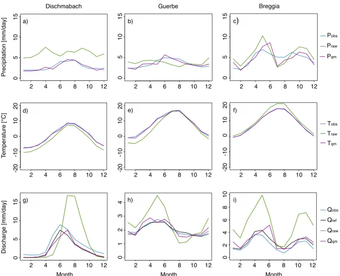
Prior to bias correction, biases in raw GCM–RCM precipitationPrawwere substantial. In our study
catch-ments, precipitation biases take the form of either a wet bias that persists primarily throughout the year (Fig. 6a) or a wet bias in the winter and spring months, often with a dry bias in the summer months (Figs. 6b,c). These main types of precipitation biases can also be seen within the other catchments not shown here. Bias-corrected pre-cipitation Pqm shows an improvement over Praw and
generally fits more closely to observed precipitationPobs.
However, biases can still remain even after bias correc-tion (seesection 4afor further discussion). Additionally, temperature biases were present. Prior to QM, the largest biases in temperatureTrawwere found in high-elevation
catchments. Within these catchments, a cold bias is evi-dent for the entire annual cycle. Lower-elevation catch-ments are less severely affected. After bias correction, temperatureTqmmatches well with observed
tempera-tureTobsirrespective of the elevation of the catchment.
The effect of these biases and bias correction on discharge depends on the elevation of the catchment.
In high-elevation catchments such as Allenbach and Dischmabach, the combination of wet biases in the winter/spring and a general cold bias often leads to a delay in discharge (Qraw), peaking 1–1.5 months after
bothQobsandQref(Fig. 6g). The delay in discharge is
due to precipitation falling as snow in the winter months at these elevations. In addition, the magnitude of dis-charge is often much greater than bothQobsandQref,
which indicates an overestimation of snow accumula-tion. After QM, the cold biases are most often improved (Fig. 6d), and the wet precipitation bias in the winter and spring months is generally reduced (Fig. 6a). Therefore, both the timing and the magnitude of the resulting
FIG. 4. Discharge for the time period of 1980–2009 for (a) the Dischmabach catchment and the GCM–RCM (CNRM-CM5–CLM4-8-17), (b) the Guerbe catchment and GCM–RCM (CNRM-CM5–RCA4), and (c) the Breggia catchment and GCM–RCM (HadGEM2-ES–RCA4). Ten simulations, which stem from the 10 parameter sets, are shown for each of the following:Qref,Qraw, andQqm.
discharge (Qqm) matches more closely with both Qobs
andQref(Fig. 6g).
In low- to medium-elevation catchments (679–1252 m MSL) such as Breggia, Sitter, and Murg, cold biases were less pronounced (Figs. 6e,f), but wet biases were often found (Figs. 6b,c). Depending on the catchment, these biases either persisted throughout the year or only impacted the winter and spring months, often with a dry bias in the summer months. This results in a bias in the magnitude of the discharge; however, timing in these mid- to low elevations is less affected compared to the high-elevation catchments (Figs. 6h,i).
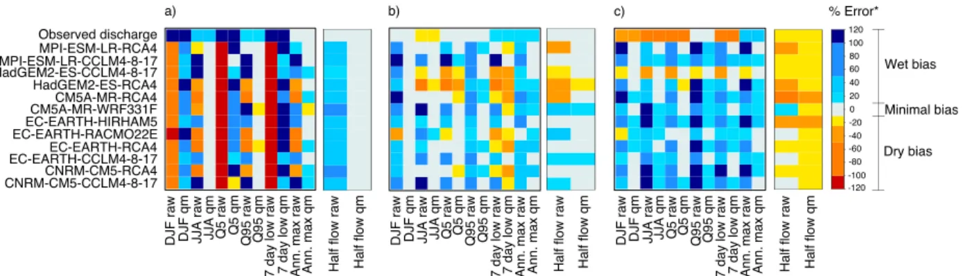
A comparison of Erawto Eqm is plotted side by side
(noted as ‘‘variable’’ with raw or qm) inFigs. 7a–c. In the majority of cases, QM leads to a decrease of bias in hy-drological variables: a striped pattern is visible when QM
and raw results are displayed side by side (e.g., Q95 col-umns;Figs. 7a–c). This striped pattern indicates relatively high versus low percent error when comparing raw to QM simulations. Overall, QM increases the agreement ofPandTtime series with observations, which leads to an improvement of the runoff time series simulated by HBV. However, there are instances where QM does not result in an improved hydrologic performance (i.e., instances where the striped pattern is not present; see
Fig. 7a, DJF columns). An explanation is that the rel-ative percent error is very sensitive in low-flow metrics where small discharge values are compared to one another. Occasionally, such small differences can result in large relative errors. However, when compared to errors over the rest of the year, the errors over winter are rather small in absolute terms.
After QM, discharge (Qqm) tends to resembleQref
more than Qobs (Fig. 8). This pattern is due to the
calibration of HBV that uses the MeteoSwiss gridded product as forcing data and the QM of GCM–RCM data that uses the same MeteoSwiss data (Pobs and
Tobs) as reference for the bias correction. Figure 8a
shows discharge for Dischmabach catchment, which is a catchment wherePqmandTqmfit the annual cycle
generally well (Figs. 6a,d). Because of the improve-ments in the representation of precipitation through-out the annual cycle, discharge is greatly improved; note that Qqm resembles Qref more so than Qobs
(Fig. 8a;section 4c). Discharge for the Breggia catch-ment (Fig. 8c) has a precipitation cycle that peaks twice within the annual year (Fig. 6c). QM improves the GCM–RCM precipitation cycle (Pqm), although
negative biases remain in the summer months. The improvements of discharge were substantial for the Guerbe catchment. The Guerbe catchment has small differences in the annual cycle of precipitation, which is relatively difficult for an annual QM method to improve. The improvements seen in discharge are a testament to the seasonal bias correction performed. The Breggia and Dischmabach catchments demonstrate the tendency for
Qqmto resembleQrefrather thanQobs. For the Guerbe
catchment,QobsandQrefare very similar, and thusQqm
resembles both.
b. Evaluating overall effect of quantile mapping
After exploring the impacts of QM for individual basins, we analyzed the impacts of QM in all catchments.
Figure 9shows whether QM leads to an improvement
FIG. 6. The long-term mean monthly (a)–(c) precipitation, (d)–(f) temperature, and (g)–(i) discharge for three example catchments. The data from one GCM–RCM are used for each catchment. (left) Dischmabach catchment, CNRM-CM5–CLM4-8-17; (center) Guerbe catchment, CNRM-CM5–RCA4; and (right) Breggia catchment, HadGEM2-ES–RCA4. All figures are for the period 1980–2009. Note the different axis scale for the three discharge plots in (g)–(i).
(warm colors) or degradation (cool colors) of the hy-drological simulations (i.e., it shows the difference be-tween the absolute value ofErawand absolute value of
Eqmfor each variable and climate model). The overall
color pattern is predominantly warm tones, which implies that QM has a generally beneficial impact on discharge metrics. In 91% of all instances (all GCM– RCMs, catchments, and metrics considered), QM was found to improve discharge. By separating out high-flow metrics (JJA, Q95, annual maximum) from low-flow metrics (DJF, Q5, 7-day low flow), we found that high-flow metrics show generally greater improvement (96% improvement rate) from quantile mapping compared to low-flow metrics (87% improvement rate). Although low-flow metrics clearly did not improve as much as high-flow metrics, the initial calculation ofErawandEqm
was very sensitive, especially when small values were compared to one another. Therefore, discharge can overall be greatly improved after QM, while low-flow metrics still show degradation, as, for instance, in the case in the Dischmabach catchment inFig. 9.
c. Ranking climate models
To synthesize our results, raw and quantile mapped GCM–RCMs were ranked according to the per-formance of runoff simulations, which are based on the precipitation and temperature extracted from the GCM–RCMs. To synthesize our results, we combined all of the hydrological variables into a single metric, referred to as ‘‘All metrics.’’ The calculation of All metrics entails taking the median across all of the hy-drological metrics (besides the half-flow date, which has a different unit) and all of the catchments for a particular GCM–RCM. The median was chosen in order to prevent the ranking from being overly affected by a particularly poor performing metric or catchment (e.g., low-flow metric).
Figure 10shows the ranking based onEraw(Fig. 10a)
andEqm(Fig. 10b), whereErawandEqmrepresent the
median of all catchments. Observed discharge is also shown in the ranking for reference, based onEobs. The
order of the GCM–RCMs along theyaxis was determined based on the ranking of the All metrics column. Within
FIG. 8. Discharge for the (a) Dischmabach, (b) Guerbe, and (c) Breggia catchments with all GCM–RCMs shown for the period 1980–2009. FIG. 7. Three example catchments are shown: (a) Dischmabach, (b) Guerbe, and (c) Breggia to demonstrate the overall impact of quantile mapping as well as the range in performance of the GCM–RCMs (yaxis) according to hydrological metrics (xaxis). The colors in the larger heat maps illustrate the values ofEobs,Eraw, orEqm(values in percent error). The colors in the smaller (half flow) heat maps are in units of days (see the * in the color bar legend). The top row within the heat plots shows observed discharge for comparative purposes. Observed discharge was not quantile mapped, thus the raw and quantile mapped columns are the same for this row.
Fig. 10a, observed discharge ranks high in comparison to the GCM–RCMs, which is in strong contrast toFig. 10b, where observed discharge ranks last. The switch in place-ment of observed discharge is due to the general im-provement of the GCM–RCM performance after quantile mapping. It is especially noteworthy that withinFig. 10b, the ranking of observed discharge is worse than any GCM– RCM forcing. The result inFig. 10bshows that after QM, the percent error betweenQqmandQrefis smaller than the
percent error betweenQobsandQref. This pattern is caused
by both the bias correction of the GCM–RCM tempera-ture and precipitation as well as the calibration of HBV since the calibration of HBV was done so thatQrefshould
resembleQobs(see section 4cfor more discussion). The
rank of Qobs as last compared to bias-corrected GCM–
RCMs is a confirmation of the ability of QM to improve discharge metrics. In addition, GCM–RCMs also change their rank betweenFigs. 10a and 10b, despite the uniform application of QM. This is in part because the differences between the bias-corrected GCM–RCMs are reduced
and a single percent error can change the order of ranking. Results show there is no general pattern pointing to a de-cidedly single-best GCM or RCM.
Besides noting the performance order of GCM– RCMs as seen inFig. 10, it is also important to show the amount of improvement (in percent error) one would achieve if choosing between the top and the lowest-ranked GCM–RCM or between QM and raw GCM– RCM data. Figure 11 shows a bar graph comparing quantile mapped discharge data (Eqm) to raw (Eraw)
discharge data for All metrics. Raw GCM–RCMs show more variability with percent errors ranging from 26% to 88%. Quantile mapped GCM–RCMs range from 4% to 11%. QM clearly reduces differences between Qref
andQqm. Note that the reduction in overall bias also
causes discharge stemming from different GCM–RCM forcings to resemble one another (see section 4c for more discussion). Figure 11 demonstrates this result, where the ‘‘All metrics quantile mapped’’ color bars show similar levels of percent error.
FIG. 9. Heat plot showing the difference (in absolute value) between the relative errors of dischargejEraw-Eqmjaccording to various metrics.
The columns correspond to the GCM-RCM simulations in the order shown inFig. 7[e.g., the first column within the Allenbach section corresponds to the GCM-RCM (CNRM-CM5-CCLM4-8-17), and the last column within the Allenbach section corresponds to ‘‘Observed discharge’’].
FIG. 10. (a) Raw and (b) QM GCM–RCMs (yaxis) ranked according to their performance for various hydro-logical metrics (xaxis) across all catchments. The placement of the GCM–RCMs along theyaxis is determined by their rank within the All metrics column. Note that observed discharge ranks high in (a) and ranks low in (b).
4. Discussion
a. How do RCM biases impact the representation of hydrological processes?
Biases in EURO-CORDEX data can be significant at the catchment scale and can have substantial effects on the simulated discharge. Our study identified wet precipitation biases, occurring in the winter/spring months with occa-sional dry biases in the summer months, as well as generally cold temperature biases, especially at high elevations. Previous studies such asFrei et al. (2018), who examined precipitation from EURO-CORDEX RCMs over the Al-pine region, found that prior to bias correction, snowfall amounts at high elevations can be considerably over-estimated. Wet precipitation biases over Switzerland have also been found in earlier GCM–RCM model generations (ENSEMBLES;van der Linden et al. 2009) as shown by
Fischer et al. (2012)andAddor et al. (2016). Our study identified that, within high-elevation catchments, the com-bination of excessive precipitation with a cold bias trans-lates into greater discharge values and delays in spring melt. Temperature biases are not as strong in low- to mid-elevation catchments and thus, in these catchments, the timing of discharge (using raw GCM–RCM data to force HBV) resembles that ofQobsandQrefrelatively closely.
Our results confirm the general beneficial use of quantile mapping, which has been reported in previous studies (Themeßl et al. 2011a;Teutschbein and Seibert
2012;Räisänen and Räty 2013). However, after the
ap-plication of a seasonal QM, biases are often still present, although reduced. This is not surprising, as previous
literature has pointed out.Addor and Seibert (2014)show that after performing a bias correction of precipitation over a daily time step, for instance, discrepancies between the observations and the GCM–RCM simulations can remain for other time scales. Our work shows a similar manifestation of this concept in that daily bias-corrected precipitation and temperature data contain biases on the monthly time scale (Figs. 6a–f). In addition, the discharge metrics used herein (Figs. 7a–c) are sensitive to various time scales. Discharge itself is the end result of processes covering a wide range of time scales. Therefore, it can be expected that discharge biases can remain even after a seasonal bias correction has been applied to GCM–RCM temperature and precipitation. Other instances where QM did not lead to an improvement in discharge simu-lations (seeFig. 7a, DJF qm or Q5 qm columns) occur when biases were not significant to start with. In partic-ular, biases in the low-flow period in high-elevation catchments can increase after QM, but the associated volume of water is typically low. In other words, although they can be large relative biases, they are not necessarily significant in absolute terms. Overall, both the magnitude and timing of discharge are improved (i.e., QM causes
Qqmto more closely resembleQobsandQref).
There are of course limitations related to any bias correction method. Within this study, a univariate bias correction was used, which means that temperature and precipitation were corrected independently of each other. This method is limited in that it does not specifi-cally consider the intervariable dependence structure between temperature and precipitation. In addition, we
FIG. 11. Raw (dark gray) and QM (light gray) GCM–RCMs (xaxis) and their median performance across all hydrological metrics (i.e., All metrics) and all catchments (yaxis).
applied quantile mapping at the daily time scale, al-though biases also exist over other time scales (e.g., decadal, subdaily). More advanced methods exist to accommodate for these factors, such as the multivariate recursive quantile nesting bias correction (MRQNBC;
Mehrotra and Sharma 2016), which corrects individual variable attributes that lead to correction of dependence biases between multiple variables. This method also corrects for lag-1 dependence and cross-dependence attributes over multiple time scales. Another promis-ing method to correct for biases on multiple time scales is the frequency bias correction method (FBC;Nguyen et al. 2016), which corrects for biases in the frequency domain. While other bias correction methods exist, the goal of this study was not to compare or advocate for a particular bias correction method. Rather, we demon-strate that the utilization of hydrological modeling can be used to evaluate climate simulations and assess whether a bias correction technique was successful at reducing the biases relevant for hydrological impact studies.
b. How does quantile mapping deal with the snow towers built by some climate models?
Some GCM–RCM biases clearly indicate that the simulations are physically unrealistic (e.g., snow depth of over 200 m at the end of the historical simulation ending in 2005). The question then arises whether it is meaningful to perform bias correction or whether the model should be excluded from the ensemble. For in-stance, the excessive buildup of GCM–RCM snow depth within some simulations provides a testing ground to investigate the sensitivity of discharge to input derived from snow tower affected simulations. Terzago et al. (2017)explored SWE in the Alps and used various ob-servational SWE datasets to evaluate CMIP5 GCM and EURO-CORDEX RCM simulations. Their study identified some extremely high values of SWE, origi-nating from excessive accumulation of snow. They chose to eliminate these climate models from the rest of their analysis. Besides the particular models that build snow towers,Terzago et al. (2017)report that all RCMs sim-ulate more SWE, along mountain ridges, than any of the reference datasets they considered. They partly attri-bute this bias to the higher resolution of the RCMs compared to the resolution of the reference datasets. Higher resolution allows for better representation of heterogeneous mountain topography and therefore for colder temperatures at high elevation. In addition, the large SWE values from the RCMs can also be explained by cold (e.g., RACMO22E) and wet biases (HIRHAM5) in relation to observations. Figure 10
shows that the ranking for all catchments considered, a
GCM–RCM with a snow tower (EC-EARTH– RACMO22E) ranks high in comparison to other GCM–RCMs. However, most catchments do not have snow towers associated with them. When considering a single catchment that has a snow tower (e.g., Allenbach catchment), the EC-EARTH–RACMO22E also ranks high. This simple analysis shows that the presence of a snow tower within a GCM–RCM does not necessarily affect temperature and precipitation (over the historical period) to the point that resulting streamflow simula-tions can detect the presence of a snow tower. However, the feedback between a snow tower and temperature over the future period has been shown to further reduce the climate change signal (Frei et al. 2018). Therefore, in the case of snow tower–affected GCM–RCMs, the per-formance of a GCM–RCM over both the historical pe-riod and the future should be considered when deciding whether a model is viable for use or not. The brief analysis of snow tower–affected GCM–RCMs herein points to the need for a greater dialogue regarding which types of biases should warrant inclusion/exclusion within a climate model ensemble.
c. The value of GCM–RCM ranking using hydrological modeling
Hydrological modeling allows for a combined assessment of the hydrologically important aspects of precipitation and temperature time series. This study provides a ranking that simultaneously considers a multitude of factors relevant for hydrological modeling (Fig. 10). The value of such a ranked set of GCM–RCMs strongly depends on the in-tended use of the ranking.
For the evaluation of climate model simulations, ranking raw GCM–RCMs according to hydrological performance provides a new perspective on climate model realism. By considering discharge metrics as a standard from which to rank and assess the performance of climate models, one can automatically account for interactions between atmospheric variables (PandT) at the catchment scale, including both linear and nonlinear hydrological processes.
For the selection of climate models for impact modeling, it is important to underline that QM largely improves the simulated discharge from a hydrological model. We found that across all GCM–RCMs, catchments, and discharge metrics, QM led to improvement of the simulations in 91% of the cases. QM simulations should therefore be consid-ered as more reliable by end users (e.g., water managers) than hydrological projections driven by raw climate sim-ulations. Another key result of this study is that QM causes the streamflow simulations to converge (see, e.g.,Fig. 8).
As Fig. 10b shows, after QM, all GCM–RCMs
the needs of the user. It is important to note that we assess climate models under current climate and do not consider their skill under future climate. Under future conditions, the spread among the bias-corrected simulations will be greater than under current conditions and should be ac-counted for when selecting GCM–RCMs. Finally, climate model selection should also be informed by the errors in hydrological metrics most relevant to the end users.
It is important to recognize that although the observed precipitation dataset (RHiresD) has a nominal resolution of about 2 km, its effective resolution is significantly coarser at 15–20 km. RHiresD is the finest precipitation dataset currently available over Switzerland, yet the catchment sizes are subgrid to its effective grid, meaning that RHiresD does not fully resolve the precipitation events in our study catchments. An implication is that catchment-scale precipitation estimates are more un-certain than what might be inferred based on the 2-km grid RHiresD data. These uncertainties can influence the ranking of the GCM–RCMs, since in some cases, GCM– RCMs may capture precipitation more realistically than RHiresD and with our setup, these GCM–RCMs would be penalized (Gómez-Navarro et al. 2012; Addor and
Fischer 2015; Prein and Gobiet 2017). Another issue arises given that the study catchment sizes are all smaller than one entire RCM grid cell. This makes the evaluation and ranking of raw GCM–RCM output challenging since these models were not designed to represent features at the spatial scale at which they are being evaluated. To help alleviate this issue, the effects of elevation on tem-perature and precipitation were explicitly accounted for prior to the ranking of the raw GCM–RCM data. For future work, a way to overcome these issues would be to work with larger catchments, but then the risk of per-turbation of the hydrological time series because of hu-man interventions would be higher than in the research catchments considered here.
5. Conclusions
This study investigated how biases in EURO-CORDEX GCM–RCM simulations impact the repre-sentation of hydrological processes. Quantile mapping
improvements over the rest of the discharge cycle. Our study demonstrates that hydrological modeling can be used to evaluate and rank climate model simulations in an integrated way at the catchment scale. For climate modelers, it is a way to gain novel insights into climate model realism. For impact modelers, who have to select climate models for hydrologic modeling, this evaluation approach is a way to assess the sensitivity of hydrological simulations to known biases, such as the existence of snow towers in some EURO-CORDEX simulations.
Another key finding of this study is that applying QM causes the convergence of hydrological simulations driven by GCM–RCMs under current climate. This stems from the use of a common reference observational dataset for the bias correction of the simulated atmospheric forcing. Since the cumulative distribution of GCM–RCM tem-perature and precipitation is forced to mimic that of the observations, it causes the resulting hydrological simula-tions to resemble each other under current climate. This implies that the ranking of GCM–RCM simulations after QM provides limited insights. Rather, ranking GCM– RCMs prior to bias correction is recommended, especially when performed over catchments that are large in com-parison to the resolution of the RCM grid. At this stage, it is unclear whether QM will cause a convergence of the future climate change impacts on discharge. Next steps include the application of this analysis to operational decision-making, which will include the consideration of future climate change impacts on hydrology.
The use of hydrological modeling to assess the per-formance of climate models has received little attention so far. Our combination of the newest generation of GCM–RCM simulations within a hydrological frame-work allows for the simultaneous consideration of a wide range of climate models, hydrologic regimes, and streamflow variables. Hydrological modeling provides new insights to climate modelers and end users and represents a novel way to assess the realism and support the selection of climate models.
Acknowledgments. This study was funded by the Swiss National Science Foundation via the SNF Grant 200020_156606: Hydrological climate change impact
assessment—Addressing the uncertainties (HIMAUI). We thank Marc Vis for support related to HBV, Sven Kotlarski for providing useful insights into CORDEX data, and the two anonymous reviewers for their com-ments. We acknowledge the Swiss Federal Offices for the Environment (FOEN), the Meteorology and Cli-matology Offices of Switzerland (MeteoSwiss), and the European Coordinated Regional Downscaling Experi-ment (EURO-CORDEX) for the hydrological, atmo-spheric, and climate modeled data, respectively.
REFERENCES
Addor, N., and J. Seibert, 2014: Bias correction for hydrological impact studies - beyond the daily perspective.Hydrol. Pro-cesses,28, 4823–4828,https://doi.org/10.1002/hyp.10238. ——, and E. M. Fischer, 2015: The influence of natural variability
and interpolation errors on bias characterization in RCM simulations. J. Geophys. Res. Atmos., 120, 10 180–10 195, https://doi.org/10.1002/2014JD022824.
——, M. Rohrer, R. Furrer, and J. Seibert, 2016: Propagation of biases in climate models from the synoptic to the regional scale: Implications for bias adjustment.J. Geophys. Res. At-mos.,121, 2075–2089,https://doi.org/10.1002/2015JD024040. Bergström, S., 1976:Development and Application of a Conceptual
Runoff Model for Scandinavian Catchments. Norrköping, 134 pp.
Criss, R. E., and W. E. Winston, 2008: Do Nash values have value? Discussion and alternate proposals.Hydrol. Processes,
22, 2723–2725,https://doi.org/10.1002/hyp.7072.
Fischer, A. M., A. P. Weigel, C. M. Buser, R. Knutti, H. R. Künsch, M. A. Liniger, C. Schär, and C. Appenzeller, 2012: Climate change projections for Switzerland based on a Bayesian multi-model approach.Int. J. Climatol.,32, 2348– 2371,https://doi.org/10.1002/joc.3396.
Fowler, H. J., S. Blenkinsop, and C. Tebaldi, 2007: Linking climate change modelling to impacts studies: Recent advances in downscaling techniques for hydrological modelling. Int. J. Climatol.,27, 1547–1578,https://doi.org/10.1002/joc.1556. Frei, C., 2014: Interpolation of temperature in a mountainous
re-gion using nonlinear profiles and non-Euclidean distances.Int. J. Climatol.,34, 1585–1605,https://doi.org/10.1002/joc.3786. ——, and C. Schär, 1998: A precipitation climatology of
the Alps from high-resolution rain-gauge observations. Int. J. Climatol.,18, 873–900, https://doi.org/10.1002/(SICI)1097-0088(19980630)18:8,873::AID-JOC255.3.0.CO;2-9. Frei, P., S. Kotlarski, M. A. Liniger, and C. Schär, 2018: Future
snowfall in the Alps: Projections based on the EURO-CORDEX regional climate models.Cryosphere,12, 1–24,https:// doi.org/10.5194/tc-12-1-2018.
Gleckler, P. J., K. E. Taylor, and C. Doutriaux, 2008: Performance metrics for climate models. J. Geophys. Res.,113, D06104, https://doi.org/10.1029/2007JD008972.
Gómez-Navarro, J. J., J. P. Montvez, S. Jerez, P. Jimé nez-Guerrero, and E. Zorita, 2012: What is the role of the obser-vational dataset in the evaluation and scoring of climate models? Geophys. Res. Lett., 39, L24701, https://doi.org/ 10.1029/2012GL054206.
Gudmundsson, L., 2016: Qmap: Statistical transformations for post-processing climate model output. R package, version 1.0-4, https://cran.r-project.org/web/packages/qmap/index.html.
——, J. B. Bremnes, J. E. Haugen, and T. Engen-Skaugen, 2012: Technical Note: Downscaling RCM precipitation to the sta-tion scale using statistical transformasta-tions—A comparison of methods.Hydrol. Earth Syst. Sci.,16, 3383–3390,https:// doi.org/10.5194/hess-16-3383-2012.
Johnson, F., and A. Sharma, 2015: What are the impacts of bias correction on future drought projections?J. Hydrol.,525, 472– 485,https://doi.org/10.1016/j.jhydrol.2015.04.002.
Jury, M. W., A. F. Prein, H. Truhetz, and A. Gobiet, 2015: Eval-uation of CMIP5 models in the context of dynamical down-scaling over Europe.J. Climate,28, 5575–5582,https://doi.org/ 10.1175/JCLI-D-14-00430.1.
Kotlarski, S., and Coauthors, 2014: Regional climate modeling on European scales: A joint standard evaluation of the EURO-CORDEX RCM ensemble.Geosci. Model Dev.,7, 1297–1333, https://doi.org/10.5194/gmd-7-1297-2014.
Li, C., E. Sinha, D. E. Horton, N. S. Diffenbaugh, and A. M. Michalak, 2014: Joint bias correction of temperature and pre-cipitation in climate model simulations.J. Geophys. Res. At-mos.,119, 13 153–13 162,https://doi.org/10.1002/2014JD022514. Lindström, G., B. Johansson, M. Persson, M. Gardelin, and S. Bergström, 1997: Development and test of the distributed HBV-96 hydrological model.J. Hydrol.,201, 272–288,https:// doi.org/10.1016/S0022-1694(97)00041-3.
Maraun, D., 2013: Bias correction, quantile mapping, and downscaling: Revisiting the inflation issue. J. Climate, 26, 2137–2143,https://doi.org/10.1175/JCLI-D-12-00821.1. Mehrotra, R., and A. Sharma, 2016: A multivariate
quantile-matching bias correction approach with auto- and cross-dependence across multiple time scales: Implications for downscaling. J. Climate, 29, 3519–3539, https://doi.org/ 10.1175/JCLI-D-15-0356.1.
Mendlik, T., and A. Gobiet, 2016: Selecting climate simulations for impact studies based on multivariate patterns of climate change. Climatic Change, 135, 381–393, https://doi.org/ 10.1007/s10584-015-1582-0.
MeteoSwiss, 2010: SwissMetNet: Ein Messnetz für die Zukunft. MeteoSwiss, https://naturwissenschaften.ch/service/news/77197-swissmetnet—ein-messnetz-fuer-die-zukunft.
——, 2013a: Documentation of MeteoSwiss grid-data products: Daily precipitation (final analysis): RhiresD. MeteoSwiss, 4 pp., https://www.meteoswiss.admin.ch/content/dam/ meteoswiss/de/service-und-publikationen/produkt/raeumliche-daten-niederschlag/doc/ProdDoc_RhiresD.pdf.
——, 2013b: Daily mean, minimum and maximum temperature: TabsD, TminD, TmaxD. MeteoSwiss, 4 pp.,https://www. meteoswiss.admin.ch/content/dam/meteoswiss/de/service-und-publikationen/produkt/raeumliche-daten-temperatur/doc/ ProdDoc_TabsD.pdf.
Nash, J. E., and J. V. Sutcliffe, 1970: River flow forecasting through conceptual models part I — A discussion of principles.
J. Hydrol.,10, 282–290,https://doi.org/10.1016/0022-1694(70) 90255-6.
Nguyen, H., R. Mehrotra, and A. Sharma, 2016: Correcting for systematic biases in GCM simulations in the frequency do-main. J. Hydrol.,538, 117–126, https://doi.org/10.1016/ j.jhydrol.2016.04.018.
Pechlivanidis, I. G., J. Olsson, D. Sharma, T. Bosshard, and K. C. Sharma, 2015: Assessment of the climate change impacts on the water resources of the Luni Region, India.Global NEST J.,17, 29–40,https://doi.org/10.30955/gnj.001370.
Prein, A. F., and A. Gobiet, 2017: Impacts of uncertainties in European gridded precipitation observations on regional
https://doi.org/10.1002/joc.1540.
Schaefli, B., B. Hingray, and A. Musy, 2007: Climate change and hy-dropower production in the Swiss Alps: Quantification of potential impacts and related modelling uncertainties.Hydrol. Earth Syst. Sci.,11, 1191–1205,https://doi.org/10.5194/hess-11-1191-2007. Schwarb, M., 2000: The alpine precipitation climate: Evaluation
of a high-resolution analysis scheme using comprehensive rain-gauge data. Ph.D. dissertation, Swiss Federal Institute of Technology, 131 pp.
Seibert, J., 2000: Multi-criteria calibration of a conceptual runoff model using a genetic algorithm.Hydrol. Earth Syst. Sci.,4, 215–224,https://doi.org/10.5194/hess-4-215-2000.
——, and M. J. P. Vis, 2012: Teaching hydrological modeling with a user-friendly catchment-runoff-model software package. Hy-drol. Earth Syst. Sci.,16, 3315–3325,https://doi.org/10.5194/ hess-16-3315-2012.
Terzago, S., J. Von Hardenberg, E. Palazzi, and A. Provenzale, 2017: Snow water equivalent in the Alps as seen by gridded
and its impact on the climate change signal.Climatic Change,
112, 449–468,https://doi.org/10.1007/s10584-011-0224-4. van der Linden, P., J. F. B. Mitchell, and P. Gilbert, 2009:
ENSEMBLES: Climate change and its impacts: Summary of research and results from the ENSEMBLES project. P. Van Der Linden and J. F. B. Mitchell, Eds., Met Office Hadley Centre, 160 pp.
Wilcke, R. A. I., and L. Bärring, 2016: Selecting regional cli-mate scenarios for impact modelling studies. Environ. Modell. Software, 78, 191–201, https://doi.org/10.1016/ j.envsoft.2016.01.002.
——, T. Mendlik, and A. Gobiet, 2013: Multi-variable error cor-rection of regional climate models.Climatic Change,120, 871– 887,https://doi.org/10.1007/s10584-013-0845-x.
Zehe, E., and M. Sivapalan, 2009: Threshold behaviour in hydro-logical systems as (human) geo-ecosystems: Manifestations, controls, implications.Hydrol. Earth Syst. Sci.,13, 1273–1297, https://doi.org/10.5194/hess-13-1273-2009.