GRASS 6 in a nutshell
by Markus Neteler
(neteler at itc dot it)
Material prepared for:
Open Source Geospatial ’05 Conference, June 16-18, 2005
University of Minnesota, Minneapolis, MN USA
http://mapserver.gis.umn.edu/mum/mtg2005.html
June 16 Workshop, 8:00 - 12:00
Title: Open Source Geoinformatics with GRASS GIS
Presenters: Markus Neteler, Kristen Perry
Contents Preface
Today, Free and Open Source Software has become synonymous with innovation and progress. Free use, modification, and distribution of programs and their source code guarantee due the free exchange of ideas between users and developers and owing to appropriate licensing. GRASS (the Geographic Re-sources Analysis Support System,http://grass.itc.it) is a free and open source GIS (Geographic Information System) software package, integrated with image processing and data visualization subsys-tems. It provides many modules for raster and vector data manipulation, rendering images on screen or on paper, multispectral image geocoding and processing, point data management and general data man-agement. GRASS provides interfaces to PostgreSQL, MySQL, DBF, and ODBC-connected databases. Further, it can be connected to UMN/Mapserver, R-stats, gstat, Matlab, Octave, Povray and other soft-ware packages.
This tutorial gives a compact introduction to GRASS 6. We intend to illustrate basic function-ality of the program. For more insight into the software capabilities, see the references listed in the bibliography. The datasets used in the workshop and also this document are available from http://mpa.itc.it/markus/mum3/.
Contents
1 Introduction 4
1.1 New features in GRASS 6 . . . 4
1.2 Downloading the software . . . 4
1.3 Available documentation and sample data sets . . . 4
1.4 Structure of GRASS databases: the “GRASS Project” . . . 4
1.4.1 Creating a GRASS database . . . 5
1.4.2 Installing the sample Spearfish data set . . . 6
1.5 Multiuser capabilities for teams . . . 6
1.6 GRASS basics: command structure and user interface . . . 6
2 Benvenuto to GRASS 9 2.1 Launching Linux, login . . . 9
2.2 Linux intro in a few minutes . . . 9
2.3 Sample session: First steps . . . 10
2.3.1 Starting GRASS . . . 10
2.3.2 Starting the d.m GIS manager: loading raster and vector maps, map display . . 11
2.3.3 Saving the GIS manager settings . . . 12
2.3.4 Saving current region settings . . . 12
2.3.5 NVIZ visualization tool . . . 12
2.3.6 Online help: Help button and g.manual . . . 13
2.3.7 Using the command line . . . 14
Contents 2.3.9 QGIS: Viewing external vector and raster GIS maps (SHAPE, GeoTIFF etc) . 15
2.3.10 QGIS: Viewing PostGIS maps . . . 15
2.3.11 Creating paper maps with QGIS . . . 15
2.3.12 QGIS: Export to Mapserver mapfile . . . 15
2.3.13 Closing the GRASS session . . . 16
3 Working with own data - Import/Export/Creating Locations 16 3.1 Import of GIS data . . . 16
3.1.1 Starting GRASS with Spearfish . . . 16
3.1.2 Importing vector ESRI SHAPE files (TIGER 2000) . . . 17
3.1.3 Importing raster Erdas/IMG files (LANDSAT-7) . . . 17
3.1.4 Importing Raster GeoTIFF files . . . 18
3.1.5 Creating new GRASS locations from datasets . . . 18
3.1.6 So many GIS formats.... . . 19
3.1.7 Closing Your GRASS Session . . . 19
3.2 Creating a new location . . . 19
3.2.1 Defining a new location interactively . . . 19
3.2.2 Creating your own location from EPSG code . . . 21
4 Raster map analysis 21 4.1 Digital elevation model (DEM) analysis . . . 22
4.2 Raster map algebra . . . 22
4.3 Geocoding a scanned map (4 corner points): Topographic map 1:24000 . . . 23
4.4 Volume data processing and visualization (demo) . . . 23
5 Image processing 23 5.1 Image classification . . . 23
5.2 Image Fusion: LANDSAT-7 – Brovey transform . . . 25
6 Working with vector data 26 6.1 Vector map import . . . 26
6.2 Attribute management . . . 27
6.3 Buffering . . . 27
6.4 Extractions . . . 27
6.5 Selecting, clipping, unions, intersections . . . 28
6.6 Conversion raster-vector and vice versa . . . 28
6.7 Digitizing in GRASS . . . 29
6.8 Digitizing in QGIS . . . 29
6.9 Working with vector geometry . . . 29
7 Vector networking 30 7.1 Shortest path analysis . . . 30
8 GRASS and R-stats interface 32
8.1 Installation of the related R packages . . . 32 8.2 R-stats/GRASS sample session . . . 32
1 Introduction
1.1 New features in GRASS 6
Over the last few years a number of significant improvements have been made to GRASS. A new topological 2D/3D vector engine and support for vector network analysis were added. Attributes are now managed in SQL-based DBMS. The NVIZ visualization tool was enhanced to display 3D vector data and voxel volumes. Messages are partially internationalized (i18N) with support for FreeType fonts, including multibyte Asian characters. GRASS is integrated with the GDAL/OGR libraries to support an extensive range of raster and vector formats, including OGC-conformal Simple Features. A new display manager and integration with QGIS (http://www.qgis.org) result in improved ease of use.
1.2 Downloading the software
GRASS is available from ITC-irst in Italy (http://grass.itc.it), and from numerous mirror sites (e.g., http://grass.ibiblio.org). It can also be obtained on CDROM, as well as on KNOPPIX derivates as “Live Linux GIS”.
1.3 Available documentation and sample data sets
Books, tutorials, manuals, online courses and further documents are listed at the “GRASS Documenta-tion Project” (http://grass.itc.it/gdp/). Sample data sets to use in exploring the functionality of the system are available from the related download page (http://grass.itc.it/download/) as well as from the Neteler & Mitasova 2004 book supplement Web site (http://mpa.itc.it/grasstutor/). 1.4 Structure of GRASS databases: the “GRASS Project”
GRASS data are stored in a directory referred to as a database (also called “GISDBASE”). This directory has to be created withmkdiror a file manager before starting to work with GRASS. Within this database, projects are organized by project areas stored in subdirectories called locations. A location is defined by its coordinate system, map projection and geographical boundaries. The subdirectories and files defining alocationare created automatically when GRASS is started the first time with a newlocation.
Each location can have several mapsets. One motivation for maintaining different mapsets is to store maps related to specific project issues or subregions. Another motivation is to support si-multaneous access by several users to the map layers stored within the same location, i.e. teams
1.4 Structure of GRASS databases: the “GRASS Project”
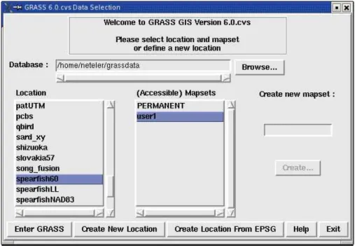
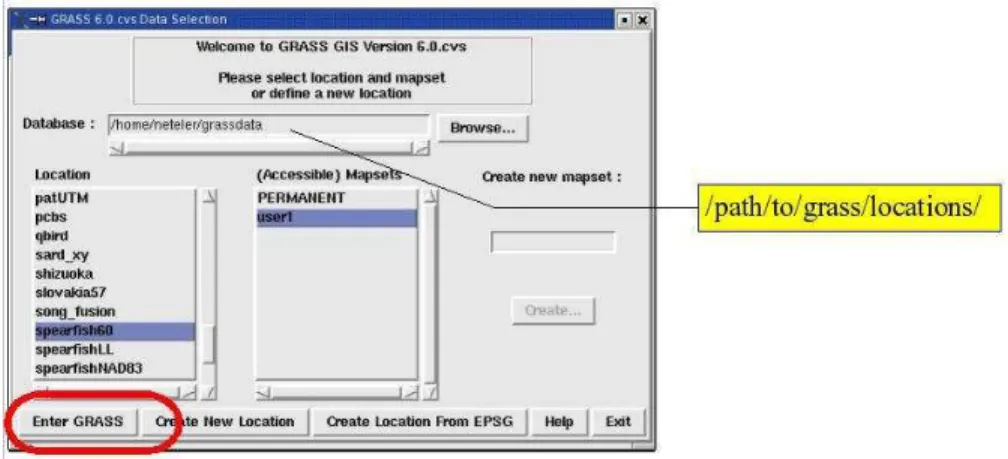
Figure 1:GRASS 6 startup screen
working on the same project. For team efforts, a centralized GRASSdatabasewould be created on a network file system (e.g. NFS). Besides access to his/her ownmapset, each user can also read map layers in other users’mapsets, but s/he can modify or remove only the map layers in his/her ownmapset. When creating a newlocation, GRASS automatically creates a special mapsetcalled PERMANENT where the core data for the project can be stored. Data in the PERMANENT mapset can only be added, modified or removed by the owner of the PERMANENTmapset, however, they can be accessed, analyzed, and copied into their ownmapsetby the other users. The PERMANENTmapsetis useful for providing general spatial data (e.g. an elevation model), accessible but write-protected to all users who are working in the samelocationas the database owner. To manipulate or add data to PERMANENT, the owner would start GRASS and choose the relevantlocationand the PERMANENTmapset. This mapset also contains the DEFAULT_WIND file, which holds the default region boundary coordinate values for the location (which all users will inherit when they start using the database). Additionally, a WIND file is kept in all mapsets for storing the current boundary coordinate values and the currently selected raster resolution. Users have the option of switching back to the default region at any time.
1.4.1 Creating a GRASS database
To create a new GRASS database, search for directory where you have write access. The disk partition should provide enough free diskspace to hold your spatial data. Create a subdirectory which represents the GRASS database (e.g., mkdir /data/grassdata/ ormkdir /home/yourlogin/grassdata/). This path has to be inserted in the “Database” line of the startup screen (see figure 1).
1.5 Multiuser capabilities for teams
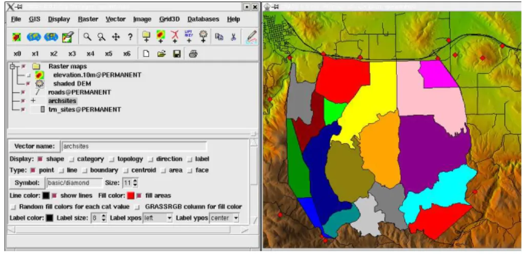
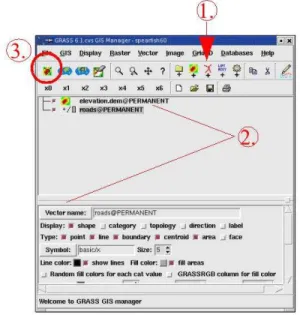
Figure 2:GRASS GIS manager with Spearfish dataset
1.4.2 Installing the sample Spearfish data set
There are a couple of sample GRASS locations available for download. In our workshop we are using theSpearfishsample dataset which must be extracted in the new database directory. Then the dataset is ready to use. Before doing so, we’ll have a quick look at the general structure of the program.
1.5 Multiuser capabilities for teams
GRASS supports teams by allowing any number of users to work in a single location (but with different mapsets) simultaneously. Users can only read maps from other mapsets if permissions are granted, but can never write to other mapsets. Maps for all group members should be stored in the PERMANENT mapset. This simple scheme permits easy management of large GIS projects.
1.6 GRASS basics: command structure and user interface
GRASS is a complete, hybrid, modularly-structured GIS with raster and vector functions. Each GIS function is managed by its own module. Thus, the system is clearly structured and appears transparent. Another advantage of this modularity is that only necessary modules are executed, which preserves system resources.
Currently three graphical user interfaces (GUI) are available in addition to the traditional command line. The default GUI is the GIS manager. The map viewer NVIZ includes support for raster, vector, volume display, animations, profiles and more (see figures 2 and 3).
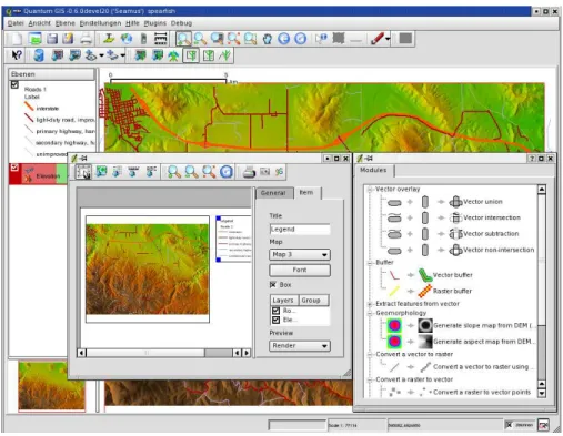
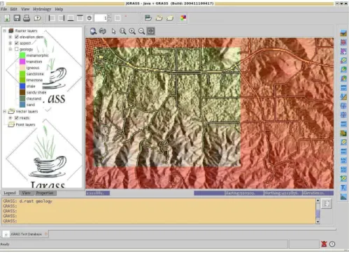
An external project, the user-friendly geodata viewer QGIS, provides direct support for GRASS. From QGIS version 0.7 onwards an extensive GRASS interface with on screen digitizer and GIS functionality is included. Also included is a new map composer tool for paper map production (see figure 4). Finally, there is JAVAGRASS (JGRASS), which is a multi-platform, multi-session GRASS framework (see figure 5). JGRASS packages GRASS to be used in production environments as opposed to research
1.6 GRASS basics: command structure and user interface
Figure 3:GRASS NVIZ viewer with satellite data
1.6 GRASS basics: command structure and user interface
Figure 5:JAVAGRASS interface
environments. The architecture of JGRASS follows a client-server model internally, separating the Graphical User Interface (GUI) from the spatial processing engine. This separation allows the easy development of remote access capabilities.
GRASS Command Overview
prefix function class type of command example
d.* display graphical output d.rast: views raster map
d.vect: views vector map
db.* database database management db.select: selects value(s) from table g.* general general file operations g.rename: renames map
i.* imagery image processing i.smap: image classifier ps.* postscript map creation format ps.map: map creation
in Postscript
r.* raster raster data processing r.buffer: buffer around raster fea-tures
r.mapcalc: map algebra
r3.* voxel raster voxel data processing r3.mapcalc: volume map algebra v.* vector vector data processing v.overlay: vector map intersections Online help in a HTML browser:g.manual <command> &
Online help in MAN format:g.manual -m <command> In the next section we show a sample session.
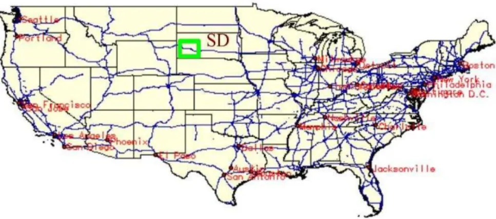
Figure 6:Spearfish, South Dakota (SD, USA)
2 Benvenuto to GRASS
In this section we are working with theSpearfish60sample data set which we extracted into the GRASS database (see above). It is located in South Dakota (SD), USA (see figure 6). Most of the maps in the Spearfish60 dataset were generated in the 1980s, with some updates and additions over the last few years. The dataset is comprised of raster and vector maps of two 1:24000 USGS quadrangles (quadrangles “Spearfish” and “Deadwood North”) and covers a major part of the Black Hills National Forest (Mount Rushmore).
2.1 Launching Linux, login
The launch of the PC system depends on the local installation. We’ll explain it during the workshop. 2.2 Linux intro in a few minutes
GRASS is a software package designed to run under various UNIX compliant systems, such as GNU/Linux, SUN-Solaris, Irix, and MacOS X, as well as under MS-WindowsNT/2000/XP (currently with Cygwin). Both 32 bit and 64 bit architectures are supported. Effective use of GRASS therefore requires certain familiarity with UNIX and adequate computer hardware. Nowadays the usage of GNU/Linux systems is rather straightforward due to the development of common graphical user inter-faces (like the KDE environment), where you can start programs from menu driven GUI environments. However, it is useful to learn how to launch commands from a terminal window (command line), as this greatly extends functionality. In particular, users can combine GRASS commands with shell and other system commands to create powerful scripts, without having to learn additional programming languages.
2.3 Sample session: First steps
Figure 7:GRASS 6 startup screen with selection of database, location and mapset
[yourname@yourmachine]
or something similar (the appearance of the prompt can be customized). Here you can enter UNIX commands and start applications. Within the terminal window, the so called “shell” interprets your commands. It receives the commands from the keyboard and transfers them to the operating system. The shell is loaded automatically when you open a terminal window. There are different shells available: C-shell (csh), bash, and the tcsh. All shells will accept every command, but they differ in their behavior, for example, how they handle cursor keys and file name completion.
Automatic file name completion saves a lot of typing because you only need to input the first character(s) of the file or command name and the shell will complete it after pressing the shell-specific completion key. The name completion key in tcsh is <ESC> (press twice), in bash it is <TAB>. Previous commands can be selected and edited with <Arrow-up> and <Arrow-down>. Also, you can transfer text from a terminal window to another one using “copy-and-paste” functions with a mouse. Use the left mouse button to mark and copy the text, then drop it wherever you need it using the middle or right mouse button (paste).
2.3 Sample session: First steps
2.3.1 Starting GRASS
Depending on the local installation you can launch GRASS 6 from either the menu or from a terminal window entering:
grass60
A graphical user interface should open as shown in figure 7.
The path to theDatabasehas to be entered into the first field. If you don’t have any existing databases, create a new directory (e.g.,grassdata/) in your home directory. For the workshop a database will be prepared and indicated. After entering the database you can either use an existingLocation(here we use “spearfish60”) or you can create a new location. We select “spearfish60” and create a newMapset
2.3 Sample session: First steps
Figure 8:GIS manager: loading a raster map Figure 9:GIS manager: loading a vector map
within the Spearfish location, by entering a new name (e.g., your login name) at the right of the startup screen and then clicking the “Create” button. The name of the new mapset will appear in the middle column; select it and then enter GRASS by clicking “Enter GRASS” at bottom left.
Some explanations:
• Adatabaseis the complete path to the GRASS database which contains one or many locations, each with its own mapsets.
• Alocationis the name of a project region.
• Amapsetis contained within the location and is used to organize the maps in folders and files by
project, by subregion, or by whatever name appears to be suitable.
2.3.2 Starting the d.m GIS manager: loading raster and vector maps, map display
The built-in GIS manager should open automatically. If not, start it with: d.m &
The additional “&” character launches the command in background, so that you can continue to enter commands into the terminal window. Now load the raster map elevation.dem and the vector map roadsas indicated in figures 8 and 9. In general you will select the map type (raster or vector), then select a map from the list, then display the map. There are options to control the map details.
Maps are displayed in a graphical map window which is called the “GRASS monitor”. You can open several monitors, they are named “x0” ... “x6”. A special monitor is the “PNG” driver which sends the contents of the monitor to a PNG file instead of displaying the maps on the screen.
2.3 Sample session: First steps
2.3.3 Saving the GIS manager settings
When you need to interrupt your work, you should first save all GIS manager settings so that you can pick up where you left off later. This is easily done bygoing to File –> Workspace –> Save as. The settings are saved as a.dm(display manager) file. This file can be reloaded into the GIS manager at a later time.
2.3.4 Saving current region settings
Since we work in a GIS, we may want to save not only maps, but also spatial settings. To make a (zoomed) region easily accessible, we can save the current spatial extent and raster resolution. For example, we can zoom into the previously displayedroadsandelevation.demmap by either using the GIS manager or by typingd.zoomat the command line (d.z<tab>should do in a bash shell). The different mouse buttons perform different operations:
Buttons:
Left: 1. corner (reset) Middle: 2. corner Right: Quit
If you have only a two-button mouse, the left and right button pressed together emulate the middle button.
Click the left button in the map to zoom. It defines the first corner of the box. You can click the left button as often as you like to find the proper first corner point for the zoom box. Then move the mouse some distance and click the middle button to define the opposite corner of the zoom box. This will zoom the displayed map(s) to the selected area. Now you can either continue like this, or exit zoom mode by clicking the right mouse button. To pan, used.zoom -pinstead, the menu will change slightly. To save a currently zoomed area as a predefined region, enter:
g.region save=roadmap
Now we want to reset the Spearfish location to its standard settings, redraw the maps and then zoom into the previously saved subregion:
g.region -dp d.redraw
g.region region=roadmap d.redraw
The monitor should display the zoomed region again.
Note that the QGIS browser comes with an intuitive zoom tool (so we don’t have to explain it here).
2.3.5 NVIZ visualization tool
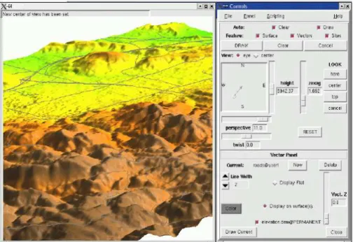
The NVIZ visualization tool is a powerful tool for graphical exploration of raster and vector maps and raster volumes (see figure 10). It permits draping maps over elevation models, stacking several maps,
2.3 Sample session: First steps
Figure 10:NVIZ visualization tool with Spearfish raster and vector maps
generation of profiles and creation of map fly-throughs. To try it out, we launch it from the command line (you can also use the GIS manager):
nviz elev=elevation.dem vect=roads
The navigation menu should be rather intuitive. The latest NVIZ software supports different view modes; some of them are similar to a flight simulator perspective.
2.3.6 Online help: Help button and g.manual
How to do this and that, you ask? Sure, often we just want to look up the parameter syntax or special hints for a command. Help can be found at different levels:
• Launching a GRASS command without parameters (in most cases) opens a graphical window: <command> e.g.,d.rast
At the bottom a HELP button is provided.
• To see available flags and parameters of a GRASS command: <command> -help e.g.,d.rast -help
• To view the manual page for a command in a web browser:
g.manual <command> e.g.,g.manual d.rast
• To view the manual page for a command in MAN style: g.manual -m <command> e.g.,g.manual -m d.rast
2.3 Sample session: First steps
Figure 11:QGIS geodata viewer with GRASS interface: Spearfish data
2.3.7 Using the command line
... you have already used it: Using GRASS on the command line means entering a command with its flags and parameters. Using shell commands, powerful scripts can be created. You may remember the file/command name completion which was mentioned earlier. It greatly enhances the speed of constructing commands! Additionally you can scroll up/down to re-use previous commands. Here some important commands:
• to open a monitor: d.mon x0
• to close a monitor: d.mon stop=x0(note: you can also simply close the window by clicking)
• to list available vector maps: g.list type=vect
• to list available raster maps: g.list type=rast
Alternate graphical user interface: QGIS
So far we have seen “pure” GRASS. But there is more to explore: Quantum GIS (QGIS). This is a stand-alone geodata browser with increasing GIS functionality. It is well interfaced now with GRASS. To launch it, just enter within (or without) a GRASS session:
2.3 Sample session: First steps
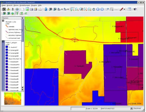
2.3.8 QGIS: Viewing GRASS maps, adding legends, labels and more
Now we will load some GRASS maps into QGIS. We load the vector maps “roads” and “fields” and the raster map “elevation.dem”. Try to replicate the view as shown in the figure 11. If you additionally load the “aspect” raster map, you can use the transparency slider to visually merge the elevation model with shades from the aspect map to generate a shaded elevation map. The slider is found when clicking with the right mouse button into the legend. Here you can also define vector legends, labels and more. The stacking order in the legend defines how the maps are displayed.
2.3.9 QGIS: Viewing external vector and raster GIS maps (SHAPE, GeoTIFF etc)
Since QGIS is a stand-alone GIS viewer, we can also load external GIS maps such as SHAPE files, GeoTIFF or ERDAS/Img files. They smoothly integrate with the GRASS data if the projections match. From QGIS 0.7 onwards vector reprojection on the fly will be supported, simplifying again the integra-tion of heterogeneous data sources.
Add some TIGER 2000 SHAPE maps and LANDSAT-7 GeoTIFF maps to your QGIS view. These files are available for the workshop, they are already reprojected from the original projections to UTM13/NAD27.
2.3.10 QGIS: Viewing PostGIS maps
If QGIS was installed with PostGIS support, we can directly load maps from a PostGIS database using theAdd PostGIS layerbutton. PostGIS is a spatial extension for PostgreSQL to store spatial (vector) objects.
If PostGIS is available, a connection can be defined withdb.connect (see the related manual page) and then an existing GRASS map copied into PostGIS withg.copy.
2.3.11 Creating paper maps with QGIS
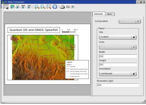
Clicking theprinterbutton brings you to the map composer tool which permits creation of a map layout for printing. Figure 12 shows the map composer window. Using theAdd new mapbutton you can insert the main view into the map composer tool. Also add a title, a vector legend and a scale. Note that the Refresh viewbutton updates the map composer contents from the main view into the composer. This is convenient if you decide to modify the map again before finalizing it. Maps can be printed, exported as EPS, SVG or high resolution PNG files.
2.3.12 QGIS: Export to Mapserver mapfile
A special feature of QGIS is the export of a current view into a UMN/Mapserver mapfile. You first construct the view with all vector legends, transparency etc., then from the main menu select: FILE –> Export Mapserver file. It even includes the paths to GRASS maps.
Figure 12:QGIS: Map composer tool
2.3.13 Closing the GRASS session
Now we close our quick-tour through GRASS and QGIS. First close the QGIS window, then the GIS manager. Finally, in the command line terminal, enter:
exit
to leave GRASS. The monitor(s) are closed automatically.
3 Working with own data - Import/Export/Creating Locations
3.1 Import of GIS data
To better illustrate daily GIS life, we will show how to import a couple of different GIS files. A set of maps has been prepared for the workshop using data from the Spearfish area.
3.1.1 Starting GRASS with Spearfish
To start GRASS with Spearfish, type grass60
At the data selection screen, select “spearfish60” from the left and your mapset from the middle column (see section 2.3.1 if you haven’t created this mapset yet). Then click “Enter GRASS”.
3.1 Import of GIS data
3.1.2 Importing vector ESRI SHAPE files (TIGER 2000)
Selected TIGER 2000 shapefiles have been prepared for the workshop (package: tiger2000_latlong_-nad83.tar.gz).
These SHAPE files are originally formatted as Latitude-Longitude/NAD83 (degree; EPSG code 4269). Before importing them into the Spearfish location, we have to reproject the maps to UTM in order to match the GRASS Spearfish sample dataset definitions (UTM zone 13N, NAD27/Clarke66; EPSG code 26713).
This can be efficiently done with theogr2ogrtool. As the original files are lacking a.prj file, which carries the projection information, we assign it on the fly using the ’-s_srs’ (source spatial reference system) parameter. The target SRS is defined with ’-t_srs’. To simplify the definition of the projections, we use EPSG code numbers which are internally expanded to the full definition. The order of command-line file specification is (maybe surprisingly) <output> <input>:
ogr2ogr -s_srs "+init=epsg:4269" -t_srs "+init=epsg:26713" \
tgr46081lkA_UTM13_nad27.shp tgr46081lkA.shp
This step must be done for all LatLong TIGER 2000 SHAPE files. You can also skip this step, as we have prepared the packagetiger2000_UTM13_nad27.tar.gz,which can be used directly. The included readme.htmlfile explains the layer names and acronyms.
Vector data are imported by usingv.in.ogr, many formats are accepted. SHAPE files are not stored in a topological format. The modulev.in.ogrcontains an internal “topology engine” which fixes a lot of common SHAPE file problems during import and generates topological information.
Now we can import the reprojected TIGER SHAPE files (shown here using the command line, you can also use the mouse by starting the command without parameters). We import the roads map (lkA) and the hydrography (lkH):
v.in.ogr tgr46081lkA_UTM13_nad27.shp out=tgr2000_roads v.in.ogr tgr46081lkH_UTM13_nad27.shp out=tgr2000_hydro d.vect tgr2000_roads col=grey
d.vect tgr2000_hydro col=aqua
To display, you can either select the imported maps in the GIS manager, use the command line or start qgisand select the maps there (using theAdd GRASS vector mapbutton).
Note: If the projection information is missing in the file (and you are sure that it corresponds to the projection of the GRASS location), you can use the ’-o’ flag to override the projection test.
3.1.3 Importing raster Erdas/IMG files (LANDSAT-7)
For the Spearfish area a LANDSAT scene has been prepared. It is already reprojected to UTM/NAD27 and subset to minimize the data size. The scene is split into three files (NIR: near infrared, MIR: middle infrared, TIR: thermal):
3.1 Import of GIS data
• spearfish_landsat7_NAD27_vis_ir.img: TM10,TM20,TM30 (blue, green, red), TM40 (NIR), TM50, TM70 (MIR)
• spearfish_landsat7_NAD27_tir.img: TM62 (TIR low gain), TM62 (TIR high gain) • spearfish_landsat7_NAD27_pan.img: TM80 (panchromatic)
In order to import raster data to GRASS, user.in.gdal(the output parameter for multichannel data is used as a prefix):
r.in.gdal -e in=<image.img> out=<image>
The module verifies that the projection of the dataset matches that of the location. If the projections do not match, an error is issued. Sometimes such definition is not present in the dataset; if you are sure that it matches the location definition, the ’-o’ flag can be used to override the test. The ’-e’ flag can be used to expand the extent of the location to match that of the dataset. However, the map is imported completely in any case. For our Spearfish example we do:
r.in.gdal -e in=spearfish_landsat7_NAD27_vis_ir.img out=tm g.rename rast=tm.6,tm.7
r.in.gdal -e in=spearfish_landsat7_NAD27_tir.img out=tm6 r.in.gdal -e in=spearfish_landsat7_NAD27_pan.img out=pan To keep the numbering right, we renametm.6to the correct numbertm.7. To look at the multichannel maps, we can generate a RGB composite on the fly:
g.region rast=tm.1 -p d.rgb b=tm.1 g=tm.2 r=tm.3
You should see the Spearfish area in near-natural colors.
3.1.4 Importing Raster GeoTIFF files
Data in the TIFF image files are either in GeoTIFF format (a single file which carries the metadata as TIFF Tags) or consist of two files, a plain TIFF filemap.tifand an ASCII filemap.tfw. A TFW, or world file, is a separate ASCII file containing the real-world transformation information used by the display software. World files can be created with any editor and also by GDAL. Make sure to get both files when not receiving GeoTIFF format. The TIFF format itself comes in several varieties, all of which are accepted by GRASS. The same LANDSAT-7 postprocessed scene we used above in ERDAS/Img format is also available as a GeoTIFF file (.tif extension). Use r.in.gdal just as you did with the ERDAS/Img LANDSAT-7 files:
r.in.gdal -e in=<map.tif> out=<map>
3.1.5 Creating new GRASS locations from datasets
Both v.in.ogr and r.in.gdal have a ’location’ parameter which can be used to generate a new GRASS location (including import of the dataset) from within an existing location. This greatly sim-plifies the procedure. Note that the dataset must include projection definitions. If lacking, ogr2ogr
3.2 Creating a new location orgdal_translatecan be used to assign the missing projection definition beforehand to the dataset (’-a_srs’ parameter).
3.1.6 So many GIS formats....
To give you an overview, there are numerous formats supported by GRASS GIS. Raster formats:
• r.in.gdal: ArcInfo, CEOS, DOQ, DTED, ENVI, Envisat, Erdas Img/LAN, FAST, (Geo)TIFF, HDF4, SAR, SDTS, ...
• r.in.bin: Binary, BIL, GMT files
• r.in.mat: MatLab files
• r.in.srtm: SRTM 1 degree tiles
Vector formats:
• v.in.ogr: SHAPE, GML, UK.NTF, SDTS, TIGER, MapInfo-File, DGN, VRT, ODBC, Post-GIS, ArcCover
• v.in.ascii: GRASS ASCII
• v.in.e00: ArcInfo E00 Format
• v.in.db: Create vectors from database with x, y[, z] coordinates
Likewise, there are also export modules to write various formats (r.out.gdalandv.out.ogr).
3.1.7 Closing Your GRASS Session
In the command line terminal, enter: exit
to leave GRASS. The display manager must be closed by you; the monitor(s) are closed automatically. So far you have seen a GRASS sample session with QGIS add-on and an import data session.
3.2 Creating a new location
3.2.1 Defining a new location interactively
Sometimes considered a tricky process, we’ll next learn to create our own GRASS locations from scratch. Remember, you can generate new locations from existing datasets automatically (see above). But it can be useful to know how to do it interactively. A major difference between GRASS and
3.2 Creating a new location other GIS is that GRASS wants the projection definitions before the user can work in a location. The advantage is that things are well defined and a mess of projection mixtures is avoided.
First you start GRASS: grass60
The welcome screen shows a couple of buttons. Click on theCreate New Locationbutton, which will take you to a text screen (someday there will be a graphical interface for this). In this screen you enter a new location name (not containing white space), and then continue by pressing “ESC”“RETURN” -i.e. press (NOT hold) the ESC key, and then press the RETURN key on your keyboard.
Below we outline the general procedure:
You will need to assign parameters to the location such as the coordinate system and datum you want to use, the project area’s boundary coordinates, and the default resolution for raster data:
• Projection: Start by chosing between, X,Y, Latitude-Longitude, UTM, or "other" coordinate
system. This choice depends on your data and the use you will make of it.
• Description: You are then prompted for a single line of text describing the project area, for
example “Topo Map of the Alps”.
• Projection details: Next you are asked for some more information about the projection. Note
that the prompts vary from projection to projection; an example follows:
– (if you chose “D - Other Projection”)specify projection name: “list” gives you the list of all available projections, examples are “tmerc” for Transverse Mercator, “lcc” for Lambert Conformal Conic, “moll” for Mollweide, etc.
– specify datum name: again use “list” to get a list of available datums, examples are “wgs84”, “nad27”, “eur79”, etc.
– Enter Central Parallel: 0 if you want the Equator as the central parallel
– Enter Central Meridian: 0 if you want the Greenwich meridian as central meridian – Enter Scale Factorat the Central Meridian: 1.0 or 0.9996 or ...
– Enter plural form of map units: for example, meters
• Area boundary coordinates: The next step is the description of the project area’s boundary
coordinates and the definition of the default raster resolution:
– The default raster resolution(GRID RESOLUTION) has to be chosen according to your needs. Generally, it is advisable to work in steps of 0.25 (0.25, 0.5, 1.75, 2.00, 12.25 etc.). This resolution does not concern vector and point data since these are stored with their exact coordinate values. Note that every raster map may have its own resolution. You can leave this screen with “ESC”-“RETURN” and then if everything is correct accept the list of parameters that appears.
Figure 13:GRASS startup screen: Creating locations from EPSG code
• You will then be taken back to the startup screen toenter the mapset’s name (if not already
entered). Another “ESC”-“RETURN” will finally let you leave this screen. This mapset is cre-ated within the new location by answering “yes” to the next question. The mapset will use the parameters of the location (such as the region and resolution definitions) as its default parameters. Now the project area, i.e. the location including a mapset, has been created. You have “arrived” in the GRASS system and can start working within this new location. Now you can verify the projection settings with:
g.proj -w
If you read this section without actually defining a new location, you may try this command in the Spearfish location.
3.2.2 Creating your own location from EPSG code
As an alternative, to create your own location in an quick and easy way, you can use the EPSG projec-tion codes. Projecprojec-tions and naprojec-tional grid systems have been standardized by the European Petroleum Survey Group (EPSG,http://www.epsg.org), giving an unique ID code to each reference system. In GRASS, they are based on the PROJ4 installation which provides an EPSG code table. Clicking on the button “Create location from EPSG” brings you to a new window (see figure 13). You will enter a new location name and the EPSG code number. If you don’t know the EPSG code, you can make use of the button that lists the PROJ4-EPSG file. Be warned that sometimes geodetic datum definitions are miss-ing here. They can be added later within the GRASS system, or you are asked in an additional window to select a datum from the available list. After entering the necessary information, click on “OK”. This will generate a new GRASS location. After that GRASS closes itself, and you have to restart it to select the newly created location. Select the location and mapset, then click the “Enter GRASS” button to launch the system.
4 Raster map analysis
GRASS is traditionally known for its powerful raster processing capabilities. All classical functionality plus time series data processing and models are available. While image processing command names
4.1 Digital elevation model (DEM) analysis differ in the first character (i.* instead of r.*), they are generally fully integrated. Any image map (from an aerial camera or satellite) can be used as a normal raster map. Additional support is available to handle multispectral maps. More sophisticated methods such as orthophoto generation and image classification are implemented as well.
GRASS supports pixelwise operations on raster maps as well as focal (neighborhood) and global (full map) calculations. Also buffers, watersheds, flow lines, slope, aspect and curvature maps can be created, and raster algebra can be performed.
To start, we want to look at the metadata of a raster map; enter: r.info <map> e.g.,r.info elevation.10m
4.1 Digital elevation model (DEM) analysis
We can calculate slope and aspect from a DEM with r.slope.aspect. First we reset the current GRASS region settings to those of the input map:
g.region rast=elevation.dem -p
r.slope.aspect el=elevation.dem as=aspect_30m sl=slope_30m d.rast aspect_30m
d.rast.leg slope_30m
Both maps are calculated in one step. Note that horizontal angles are counted counterclockwise from the East. Slopes are calculated by default in degrees. Thed.rast.legcommand adds a simple legend to the monitor.
There are additional modules which work with DEMs: depression areas can be filled withr.fill.dir, and flowlines calculated withr.flow. Watershed analysis can be done with r.watershed and, on massive grids, withr.terraflow.
4.2 Raster map algebra
GRASS provides the very powerful map calculatorr.mapcalc. This module is best used on the com-mand line as there you have flexible cursor support provided by the shell. It operates cell by cell, using a moving window technology. To start with some simple operations, we filter all pixels with elevation higher than 1000m from the Spearfish DEM:
r.mapcalc "elev_1500 = if(elevation.dem > 1500.0, \
elevation.dem, null())" d.rast elev_1500
The command, embedded in double quotes, contains an “if” statement (if higher than 1500m) with a “then” option (copy the pixel values) and an “else” option (write No Data if the condition is not satisfied). The null()function is a reserved word which inserts aNo Data value for the actual raster cell being processed. There are a couple of further functions available such asmean(), min(), max(), sin(), cos()etc. The map calculator can accept more than one input map. New maps can be generated
4.3 Geocoding a scanned map (4 corner points): Topographic map 1:24000 from calculations performed on a set of input maps. Additionally adjacent values can be considered, e.g. to generate flow through a landscape. Please refer to the manual page or the books indicated in the bibliography for further functions and examples.
4.3 Geocoding a scanned map (4 corner points): Topographic map 1:24000
GRASS can be used to geocode unreferenced (e.g., scanned) maps by defining ground control points. Such a scanned map should be imported into a XY location without projection information. This location can be automatically created when using ther.in.gdal command within another location. Using the “location” parameter the command will not only import the map, but also write it to a new location (see section 3.1.5). Then GRASS must be restarted with the new XY location containing the scanned map. We now quickly outline the procedure without going into too many details:
• The scanned map has to be inserted into an image group (i.group; even if it is just a single map).
• The group is targeted to a reference location (i.target).
• The user opens a GRASS monitor and graphically places corresponding ground control points
(i.pointsori.vpoints). The unreferenced map is loaded into the left side of the graphical display, and the reference map is loaded into the right side. For an internally undistorted map four corner points should suffice.
• The ungeocoded map is rectified into the reference location (i.rectify). The polynomial order for a 4-point rectification is 1.
Once the rectification is done, GRASS has to be left and restarted with the reference location. Now the result can be validated.
4.4 Volume data processing and visualization (demo)
A recent enhancement to GRASS is the capability to process raster volumes (voxels). This can be used to describe soil data or atmospheric data without the constraints of 2D maps. GRASS provides 3D spline interpolation and 3D map algebra as analytical tools. NVIZ was recently enhanced to dis-play volumes (e.g., isosurfaces, see figure 14). We will show examples during the workshop. The Slovakia sample location is available from the Neteler & Mitasova 2004 book supplement Web site (http://mpa.itc.it/grasstutor/, see 2ndedition datasets).
5 Image processing
5.1 Image classification
In image classification we generate a thematic map from a (set of) input channel(s). These input maps are usually aerial or satellite data. Multispectral data can be considered as a stack of raster maps with
5.1 Image classification
Figure 14:NVIZ volume visualization of Slovakia rainfall data
identical spatial reference. During the image classification procedure the spectral response of objects is analysed and assigned to classes. The resulting map contains a set of classes which may represent landuse and landcover.
GRASS supports multiple channels, they can be grouped together withi.group. Then either an auto-mated statistical analysis is done on the input channels (unsupervised classification) or training areas have to be digitized by the user to define known landuse/landcover areas (supervised classification). GRASS then derives spectral signatures for the desired classes and runs the final analysis on all pixels of all input channels, assigning each pixel to a class. In the case of unsupervised classification the classes are just numbered, in the case of supervised classification they correspond to the names of the training areas.
While the more sophisticated supervised classification is explained in the literature, we will show here a simple unsupervised classification here (Maximum Likelihood algorithm):
i.group group=lsat subgroup=lsat in=tm.1,tm.2,tm.3,tm.4,tm.5,tm.7 i.cluster group=lsat subgroup=lsat sig=sig.cluster \
5.2 Image Fusion: LANDSAT-7 – Brovey transform
Figure 15:NVIZ showing a LANDSAT-7 Brovey fusion composite
i.maxlik group=lsat subgroup=lsat sig=sig.cluster \
class=tm.class rej=tm.class.rej d.rast.leg tm.class
d.rast.leg tm.class.rej
Thetm.classmap holds the result, thetm.class.rejmap the confidence level for each pixel. 5.2 Image Fusion: LANDSAT-7 – Brovey transform
An illustrative example of visually improving a LANDSAT-7 scene can be done with the Brovey trans-formation. Here three multispectral channels (28.5m res.) and the panchromatic channel (14.25m res.) are merged in this process to three new Red, Green, Blue channels. After importing the prepared LANDSAT-7 subscene for Spearfish we run:
i.fusion.brovey -l ms1=tm.2 ms2=tm.4 ms3=tm.5 pan=pan out=brovey g.region -p rast=brovey.red
r.composite r=brovey.red g=brovey.green b=brovey.blue \
out=tm.brovey d.rast tm.brovey
The input channels have to be 2, 4, 5 and the panchromatic channel and flag ’-l’ for the LANDSAT-7 sensor. Then we set the GRASS region settings to one of the resulting high resolution channels and create a new map from the three new R, G, B Brovey channels. We can display this map using the GIS manager or QGIS. Comparing to tm.4 or other channels you can observe the improved spatial resolution.
We can also drape the result of the image fusion over the high resolution DEM with NVIZ (see fig-ure 15):
nviz elevation.10m col=tm.brovey
6 Working with vector data
GRASS 6 comes with a completely overhauled vector engine which is extended to manage 2D and 3D topological vector data. The new internal vector data format is now portable between 32bit and 64bit platforms. In addition, a new spatial indexing system accelerates vector data access and a category indexing system accelerates attribute queries. Vector data from other GIS software can be imported (allowing for topological data clean-up) as well as live-linked into the GRASS database as virtual maps. The new integratedDirected Graph Libraryprovides support for vector network analysis. Vector map overlays, intersections and extraction of features are implemented. The new vector engine includes full and flexible integration of database management systems (DBMS) for attribute management (currently DBF, PostgreSQL, mySQL, and ODBC are supported). SQL statements are used to manage attributes. Graphical updating of vector attributes has been implemented as well in the interactive vector query tool.
In this section we will explore basic vector functionality.
Supported geometry types are point, centroid, line, boundary, area (boundary + centroid), face (3D area), kernel (3D centroid), and volumes (faces + kernel). Geometry storage is true 3D: x, y, z with z=0 in the 2D case.
6.1 Vector map import
Vector maps can be imported from various sources such as ArcInfo-Coverages, CSV, DGN, SHAPE files, GML, MapInfo, MySQL, ODBC, OGDI, PostgreSQL/PostGIS, S57, SDTS, TIGER, UK .NTF, and VRT. The module for importing vector maps isv.in.ogr. The input “dsn” (data source name) parameter can be a file, a directory or a database connection, depending on the data format. As GRASS is a topological GIS, non-topological Simple Feature data such as SHAPE files are transformed into a topological representation upon import. Data quality is verified during the import, and vector features which violate topological conditions are stored in a separate layer for later inspection. For more details please refer to the manual page ofv.in.ogr.
As an example, we import a SHAPE file map generated from TIGER 2000 data into the Spearfish location and look at it:
v.in.ogr dsn=tiger_lines.shp out=tiger_lines d.vect tiger_lines
Maps can also be simply registered usingv.external. In this case only pseudo-topology is generated and the map is read-only (so no modifications can be done).
6.2 Attribute management 6.2 Attribute management
By default GRASS 6 manages vector attributes in dBase (xBase) files. To add or remove a link between a vector map and its attribute table(s), the commandv.db.connectis used. It also prints the current connection(s). We look at two maps:
v.db.connect -p roads v.db.connect -p streams
While the roads map is linked to an attribute table, the streams map lacks it.
When using an external database, the moduledb.connectis used to define the connection parameters, thendb.loginto enter the user name and the password. This is necessary for PostgreSQL and PostGIS connections and for connections to some other databases.
A set of db.* modules are available to list table names, column names and types, to make SQL queries and to create or alter table definitions. We can query the attributes of the roads map:
echo "SELECT * FROM roads" | db.select
This works for any table depending on how GRASS is connected to a (external) database (see db.connect). A more convenient way to query associated tables is to usev.db.select. For example, we can list the attributes of the roads map with:
v.db.select roads
A report containing area sizes or line lengths is generated withv.report. 6.3 Buffering
Buffering can be done for vector maps using thev.buffercommand. Here we show how to generate buffers around the archaeological sites in the Spearfish location for 300 meters:
d.vect archsites
v.buffer archsites out=archsites_buf300 buffer=300 d.vect archsites_buf300 col=red
To generate half-buffers for lines, one can usev.parallel. It adds a single, parallel line to either the left or the right side.
6.4 Extractions
Vector features can be extracted in different ways from a map: They can be selected by ID (called “cat” or “category number” in GRASS language), by attribute value via “where” SQL clauses or by geometry type (point, line, etc). As an example we can extract the interstates from the roads map by attribute. First we display the attribute table to see how it is written and how the column to be queried is named, then we extract the vector lines into a new map:
d.erase d.vect roads
6.5 Selecting, clipping, unions, intersections v.db.select roads
v.info -c roads
v.extract roads out=interstates where="label=’interstate’" d.erase
d.vect interstates
6.5 Selecting, clipping, unions, intersections
For our clipping example we import the TIGER 2000 urban areas (again within the map package tiger2000_UTM13_nad27.tar.gzfor the Spearfish area):
v.in.ogr dsn=UA_46081_UTM13_nad27.shp out=urban_areas d.vect urban_areas
We want to extract all roads which are within the urban areas. For this we usev.selectand specify the urban area polygon map and the roads line map as parameters (ainput and binput):
v.select ain=roads bin=urban_areas out=urban_roads d.vect urban_roads col=red
As a second example we want to clip the unified school districts from TIGER2000 to the urban areas which we first import. In this case we have to use a different command which permits us to use polygon maps as input:
v.in.ogr dsn=tgr46081uni_UTM13_nad27.shp out=school_dist_unified v.overlay ain=urban_areas bin=school_dist_unified \
out=urban_school_dist op=and d.vect urban_school_dist fcol=yellow To verify, we can query the newly created map:
d.what.vect urban_school_dist
There are further methods implemented in these two commands, see the manual pages for details. To extract data from a single map according to IDs or based on a SQL statement, usev.extract. 6.6 Conversion raster-vector and vice versa
GRASS is able to convert between raster and vector models (map representations), including attribute transfer. To convert vector maps to raster maps, usev.to.rast. It can either assign fixed values to the resulting map (useful when generating a raster MASK) or transfer the attributes of a specified column. The moduler.to.vectdoes the opposite, it vectorizes raster points, lines and areas. While points can be vectorized straight away, lines have to be thinned (skeletonized) withr.thinbeforehand.
6.7 Digitizing in GRASS
Figure 16:GRASS digitizer: v.digit
6.7 Digitizing in GRASS
The GRASS digitizing tool isv.digit. It has recently been completely rewritten and is now fully graphically based. The buttons should be self-explanatory. To start with a new map, the ’-n’ flag has to be added (or the button activated in the menu). Then, in the settings menu, a new attribute table can be defined, along with the snapping distance. A background map can optionally be loaded prior to beginning digitizing. Areas (currently) have to be digitized in two parts. Closed areas become green, while topologically invalid features remain red. In this case zooming is recommended to identify the error. Once a feature is digitized, a window pops up so that you can enter attributes for this feature. Figure 16 illustrates the setup.
6.8 Digitizing in QGIS
An interesting alternative is to use the digitizer within QGIS. To do so, first an empty map has to be created:
v.in.ascii -e out=newmap
Then launch QGIS within the GRASS terminal and load this new or an existing map into QGIS using the Vector/GRASS icon.
6.9 Working with vector geometry
In GRASS an area polygon is defined by a boundary + a centroid. Lines can be a (poly-)line or a boundary.
Figure 17:Native directions in GRASS vector data used for network analysis
• v.build: generate topology (automatically done), write erratic vectors to a new error map for later inspection
• v.build.polylines: make polylines of connected vector lines
• v.category: report vector IDs (called “categories” or “cats” in GRASS), automatically assign new cats to vectors, add missing centroids
• v.clean: cleans topological problems, snap nodes, remove dangles, small areas, eliminate sliv-ers, prune etc.
• v.to.db: report area side IDs of boundaries (left, right)
• v.type: convert vector geometry types (point vs. centroid; 3D point vs. kernel (3D centroid); line vs. boundary; 3D area vs. face)
• d.vect: display directions of vector lines (indicated by small arrow, see figure 17)
7 Vector networking
A new set of GRASS modules supports operations performed on vector networks. Default calculations are based on vector lengths. But it is possible to assign cost attributes to nodes and for two directions of each vector line (e.g., to simulate traffic flows).
7.1 Shortest path analysis
The connection between two positions on a vector network can be graphically analyzed with d.path. The module needs an open GRASS monitor. If no attributes are specified, only the vector line lengths are taken into consideration. We can experiment with the roads map:
7.2 Further network analysis tools
Figure 18:Shortest path calculations
The mouse buttons have to be used, they are explained in the terminal window. The calculated shortest path is immediately highlighted in the GRASS monitor (see figure 18). To save such a shortest path, thev.net.pathmodule has to be used instead.
7.2 Further network analysis tools
The following methods of vector network analysis are currently implemented in GRASS:
• v.net.path: shortest path (connection between two positions),
• v.net.salesman: traveling salesman (round trip),
• v.net.alloc: allocation of resources (create subnetworks, e.g. fire brigade),
• v.net.steiner: minimum Steiner trees (star-like connections, e.g. broadband cable)
• v.net.iso: iso-distances (from centers),
8 GRASS and R-stats interface
The interface between GRASS and R statistical language (R) is currently undergoing significant changes (Bivand, 2005). The new design is embedded in the new efforts to develop coherent spatial classes for R. The basic website for the new GRASS interface is hosted at SourceForge (http://r-spatial.sourceforge.net). The new package is named “spgrass6”. The basic spatial object classes are maintained in the “sp” package. The additional “spGDAL” class is a wrapper for func-tions in the “rgdal” package, which interfaces to the GDAL library. Another package is “spmaptools”, which is an interface to the SHAPE library.
8.1 Installation of the related R packages
Installation is done as follows (R-stats 2.1.0 or later is needed): R
> install.packages(c("sp", "rgdal", "maptools"), dependencies=TRUE) > rS <- "http://r-spatial.sourceforge.net/R"
> install.packages(c("spgrass6", "spGDAL", "spmaptools"), repos=rS, dependencies=TRUE)
> q()
8.2 R-stats/GRASS sample session
To get a feeling how the R-stats language works, we start GRASS/Spearfish for our sample session and reset GRASS to default settings, then we launch R within the GRASS terminal. A couple of commands are indicated: grass60 g.region -dp R > library(spgrass6) > G <- gmeta6()
The above commands load the interface extension and then the GRASS environment into the R session. The next command shows the environment settings:
> str(G)
8.2 R-stats/GRASS sample session > geology <- readCELL6sp("geology")
> summary(geology) > str(geology)
Since we are using GIS data, we want to look at the map:
> image(geology, "geology", col = terrain.colors(10))
To add a legend, we first control the number of classes in the geology map, then display the legend: > system("r.info -r geology")
> legend(c(590000, 605000), c(4912570, 4913850), legend = 1:9, fill = terrain.colors(10), cex = 0.8, bty = "n", horiz = TRUE) > q()
The new R/GRASS6 interface is subject to change. To keep this tutorial short, we suggest further reading elsewhere for geostatistics with R-stats. Links can be found in the Applications/Geostatistics section of the GRASS Web site.
Conclusion
This short tutorial tried to show you the power of the new GRASS 6 release. We hope that you got some insights and inspirations to use GRASS for you own work. Please visit the Web sites regularly, as development proceeds quickly. And don’t hesitate to participate, sending your comments, suggestions or even source code!
Acknowledgments
The author is grateful to Ken Boss and Kristen Perry for comments on an earlier version of this text. Bibliography
• Bivand, R., 2005, Interfacing GRASS 6 and R: Status and development direction. GRASS Newletter June 2005, Vol.3,http://grass.itc.it/newsletter/
• GDF Hannover, 2005, An introduction to the practical use of the Free Geographical Information System GRASS 6.0. Published under GNU FDL,http://www.gdf-hannover.de/literature
• Neteler, M., H. Mitasova, 2004, Open Source GIS: A GRASS GIS Approach. 2nd Edition. 424 pages, Kluwer/Springer, ISBN: 1-4020-7088-8. Online supplement: http://mpa.itc.it/grasstutor/
8.2 R-stats/GRASS sample session To appear (these books should mention GRASS as well):
• Erle, S., R. Gibson, J. Walsh, 2005, Mapping Hacks. 564 pages. 1st Edition June 2005 (est.) http://mappinghacks.com/, ISBN: 0-596-00703-5
• Mitchell, T., 2005, Web Mapping Illustrated: Using Open Source GIS Toolkits. 1st Edition June 2005 (est.), ISBN: 0-596-00865-1