Automated Morgan Keenan Classification of Observed Stellar Spectra Collected by the Sloan Digital Sky Survey Using a Single Classifier

(1)

Central Washington University

ScholarWorks@CWU

All Faculty Scholarship for the College of the

Sciences

College of the Sciences

10-17-2019

Automated Morgan Keenan Classification of Observed Stellar

Spectra Collected by the Sloan Digital Sky Survey Using a Single

Classifier

Michael J. Brice

R

ă

zvan Andonie

Follow this and additional works at: https://digitalcommons.cwu.edu/cotsfac

Part of the Artificial Intelligence and Robotics Commons, Data Science Commons, Numerical Analysis and Scientific Computing Commons, and the Stars, Interstellar Medium and the Galaxy Commons

(2)

Automated Morgan Keenan Classi

ﬁ

cation of Observed Stellar Spectra Collected by the

Sloan Digital Sky Survey Using a Single Classi

ﬁ

er

∗

Michael J. Brice and Răzvan Andonie

Computer Science Department Central Washington University Ellensburg, WA 98926, USA

Received 2019 June 22; revised 2019 August 18; accepted 2019 August 30; published 2019 October 17 Abstract

The classification of stellar spectra is a fundamental task in stellar astrophysics. Stellar spectra from the Sloan Digital Sky Survey are applied to standard classification methods, k-nearest neighbors and random forest, to automatically classify the spectra. Stellar spectra are high dimensional data and the dimensionality is reduced using astronomical knowledge because classifiers work in low dimensional space. These methods are utilized to classify the stellar spectra into a complete Morgan Keenan classification (spectral and luminosity)using a single classifier. The motion of stars (radial velocity) causes machine-learning complications through the feature matrix when classifying stellar spectra. Due to the nature of stellar classification and radial velocity, these complications cannot be corrected. However, classifiers utilizing a large set of observed stellar spectra, which has had astronomical-specific feature selection applied, performed computationally fast with extremely high accuracy.

Key words:Stellar Spectra Classification–Luminosity Classification–Morgan Keenan Classification–Automatic Classification–Redshift– Astronomical Feature Selection– K-Nearest Neighbors– Random Forest–

Imbalanced Data

1. Introduction

Stellar classification is a fundamental task in stellar astrophysics. Traditionally, stellar spectra are classified by determining the wavelengths of absorption lines using wavelet transformations, statistical analysis, and using references to the Morgan Keenan (MK) classification scheme (Morgan et al. 1943) or they are classified by comparing the best fit of the spectra to that of templates using statistical tests (Duan et al. 2009). The traditional classification schemes require complex data transformations and analysis to identify the class of a star based on its spectrum.

The amount of astronomical data and dimensionality of said data is growing rapidly through more and more ambitious astronomical surveys. The Sloan Digital Sky Survey(SDSS)is an example of an ambitious astronomical survey with high-quantity and dimensional data.

Presently, SDSS is creating the most detailed 3D maps of the universe ever made, with deep multicolor images of one-third of the sky, and spectra for more than three million astronomical objects1(York et al.2000). The SDSS provides stellar spectra with observed wavelengths. The following experiments will classify stars using the SDSS data run 14 optical spectra data set.

The SDSS and other large astronomical surveys create challenging problems for a thorough and speedy analysis. As such, automated classiﬁcation methods are explored. However, some classiﬁcation algorithms are limited to low dimensional data, making the use of feature selection and feature extraction essential.

Radial velocity(RV)creates complications for the automated classiﬁcation of stellar spectra through the feature matrix. The automated process for identifying RV and stellar class that the

SDSS uses is as follows (Bolton et al. 2012 and SkyServer: Redshifts, Classiﬁcations, and Velocity Dispersions2).

1. Redshift and classiﬁcation templates for galaxy, quasar, and cataclysmic variable (CV) and non-CV star classes are constructed by performing a rest-frame principal-component analysis (PCA; Shlens 2014) of training samples of a known redshift.

2. The combination of redshift and template class that yields the overall best ﬁt (in terms of lowest reduced chi-squared) is adopted as the pipeline measurement of the redshift and classiﬁcation of the spectrum.

3. The most common warningﬂag is set to indicate that the change in reduced chi-squared between the best and next-best redshift/classiﬁcation is either less than 0.01 in an absolute sense, or less than 1% of the best model reduced chi-squared, which indicates a poorly determined redshift.

This paper proposes a novel approach to stellar classiﬁcation characterized by the following:

1. avoids complex transformation and statistical analysis of the spectra space using machine learning;

2. uses spectra without RV corrections;

3. and uses astronomical knowledge to perform feature selection.

Stellar spectra are classified into a complete MK classifi ca-tion(spectral and luminosity)using a single classifier method. Astronomical knowledge is used to reduce the number offlux measurements. This results in key aspects of the spectra being preserved for classification which allows for a complete spectral and luminosity classification to be possible. However, the work conducted here deals with spectra with RV in the range of≈±240 km s−1.

∗_{Released on 2019 October 17.}

1

(3)

The structure of this paper is as follows. Section2describes the approach to classiﬁcation. Section 3 describes the experimental setup and the results. Section 4 provides a discussion of the results. Finally Section 5 provides the conclusions.

2. Approach to Classiﬁcation

In this section, the data preprocessing, machine-learning classiﬁers, and feature selection are described.

2.1. Data Preprocessing

The only data preprocessing required for this approach is

flux scaling using Equation(1). If a sample is known to have missing or corrupt flux measurements around the absorption lines used for feature selection, then an imputer3 method is required to fill in missing values. None of the samples in the data set used in this analysis required an imputer.

( ) = -f f f f f 1 i i ,scaled min max min

where fi is the ith ﬂux measurement, fmax and fmin are the

maximum and minimumﬂux measurements, respectively, and f_i_,scaled is the resulting scaledﬂux.

2.2. Machine Learning and Feature Selection The classiﬁer methods of k-nearest neighbors (KNN) and random forest(RF)are used in this approach. KNN classiﬁes using the k-nearest known samples. More in depth explana-tions of KNN can be found in Marsland(2015), Ivezic et al.

(2014), and Goldberger et al. (2005). RF classiﬁes using a forest of decision trees, where each tree votes on the classiﬁcation. More in depth explanations of RF can be found in Marsland(2015), Ivezic et al.(2014), and Breiman(2001). KNN and RF were chosen because they are widely used in astronomy (Yi & Pan 2010; Ivezic et al. 2014; Bai et al. 2019), and they work well in low dimensional spaces

(Breiman2001; Goldberger et al.2005). RF was also chosen because it demonstrated good results in earlier work found in Brice & Andonie (2019).

The difference between the work presented here and the work of other authors is feature selection. Feature selection is the act of taking a set of attributes or features and extracting or transforming the most relevant ones for classification and to reduce the number of dimensions for the input space for the classifier model (Bolón-Canedo et al. 2015). Authors Bazarghan & Gupta(2008), Sánchez & Prieto(2013), and Yi & Pan(2010)do not use feature selection, rather they use the full range of wavelengths. This causes the input space for the classifier models to be very large in dimension, which makes the algorithms slow. Bazarghan & Gupta (2008)rebinned the SDSS spectra to have the same resolution as the Jacoby

(Jacoby et al.1984)spectra. One could argue that this is feature selection because they are converting and reducing the number of measurements, but a more accurate description would be that they are simply spectraﬁtting and not signiﬁcantly reducing the number of dimensions. Sánchez & Prieto (2013)use K means clustering to classify SDSS stellar spectra and do not reduce the

number of dimensions. Yi & Pan(2010)utilized RF to classify stellar spectra. The authors also compared RF to neural networks(multilayer perceptron, MLP).

Authors Xing & Guo(2004), Bazarghan(2008), and Bailer-Jones et al. (1998) use PCA to reduce the number of ﬂux measurements, but they maintain the shape and structure of the overall spectrum. Xing & Guo (2004) also use a wavelet transformation to reduce noisy ﬂux measurements, but again they maintain the shape and structure of the spectrum. Others such as Zhang et al.(2008) normalized the continuum of the spectra. It is important to note that this does not reduce the dimensions of the spectra. Bai et al.(2019)uses a color space rather than spectra to classify stars. The authors use nine color bands (i.e., g−r, r−i, etc.) as their features. Elting et al.

(2008)also use photometric data instead of spectra to classify stars. Schierscher & Paunzen(2011)actually reduce the spectra using a similar approach to the work in this paper by using absorption lines, but they reduce the dimensions from 2400 to 435, where this paper reduces down to 34, as explained in Section 3. However, Schierscher & Paunzen (2011) classify effective temperature ranges and not direct spectral and luminosity classes.

From an astronomical point of view, spectra contain two features:ﬂux and wavelength. From a machine-learning point of view, spectra containNfeatures, whereNis the number of

flux measurements. In earlier work conducted in Brice & Andonie(2019), standard machine-learning feature selection methods are used which use a statistical approach to rank correlation between flux measurements and spectral classes. Then the K most correlated features(flux measurements)are taken as the input space to the classifier model. This approach does not maintain the shape or structure of the spectra. The work presented in this paper does not use machine-learning feature selection, rather astronomical knowledge of the spectra to reduce the number of dimensions in the input space.

The input space to classiﬁer models is known as a feature matrix. Each column of the feature matrix is a unique feature/ attribute/dimension of the object to be classiﬁed and the rows are the individual samples. For spectra, these features are the

ﬂux measurements, as seen in Table1. It is important to note that the wavelength values are used as the title of the unique features, not as the features themselves.

The stellar spectra found in the SDSS data set contain on average 4617ﬂux measurements or in another terms the input space has 4617 dimensions. As stated above, feature selection is used to reduce these dimensions. Standard machine-learning feature selection methods used in Brice & Andonie

(2019) did not work for these experiments because the spectral classes overshadow the luminosity classes. This means that statistical correlation between speciﬁc ﬂux

Table 1

Example of the Feature Matrix Using Two Sets of Wavelengths around Two Absorption Lines

Wavelength: Wavelength: Wavelength: Wavelength: 4095.43Å 4110.55Å 4219.88Å 4235.45Å

Spectrum 1 Flux Flux Flux Flux

Spectrum 2 Flux Flux Flux Flux

Note.The 34 features result in a 34 column feature matrix.

3

An imputer is used toﬁll in missing values in a feature matrix. Brice & Andonie(2019)utilize a moving average imputer for missing values in stellar spectra.

(4)

measurements and spectral class is stronger than the same

flux measurement and luminosity class. This is apparent because the luminosity classes are based on the width of the absorption lines, which makes it difficult for individual flux measurements to be correlated to both luminosity and spectral classes. Therefore, flux measurements around an absorption line are used rather than the ones that are statistically correlated.

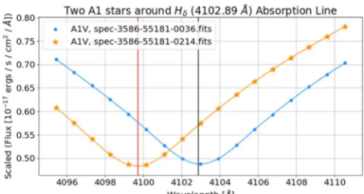
Since there is not one absorption line that all spectral classes share, two absorption line regions are used. The two absorption lines with rest vacuum wavelengths are H_δ(4102Å)and CaI

(4227Å). B and A stars have H_δ, K and M have CaI, and F and G have both absorption lines. Spectral classes are separated because of the intensity of the flux in the regions and luminosity classes are separated because of the widths of the absorption line. Figure 1 shows how the width of the absorption line changes theflux measurements for two A-type stars. Using these two regions the feature matrix can be built. The flux measurements from the H_δ region and the flux measurements from the CaI region are combined to create a single flux array per sample, as seen in Table 1. This feature selection must also be able to incorporate the shifting of the spectrum due to RV. Figure 2 shows that with a sufficiently sized region, RV can be incorporated.

The feature matrix can be represented as an N-dimensional hypercube. Where each feature is a dimension in this hypercube. As mentioned before, the wavelengths are used as dimension labels, where the ﬂux measurement at that wavelength is the magnitude of the vector in that dimension. This results in each reduced spectrum being represented as an N-dimensional point. As the shape and intensity of theﬂux in these regions change due to spectral class, the positions of these reduced spectra change in this N-dimensional hypercube. The same happens when the width of the absorption line changes with luminosity class.

A problem arises with the feature matrix because RV causes the flux measurements to be shifted in wavelength. This is illustrated in Table 2. As mentioned earlier, each feature is unique. The problem that RV causes is that it breaks this feature uniqueness. To overcome this problem, a sufficient number of samples of the exact same class with different RV that span the range of realistic RV are required. This gives the training data set for the classifier model sufficient samples of spectral and luminosity classes at different RV. In terms of KNN, this allows for sufficient neighbors to be nearby when classifying. In terms of RF, this

forces the splitting threshold of each decision tree’s node to include spectra with RV.

3. Experiments

In this section, the experimental setup is described and the results are presented.

3.1. Experimental Setup

The data set used in these experiments comes from SDSS data run 14, which was collected using the Baryon Oscillation Spectroscopic Survey (BOSS) spectrograph4

(Smee et al. 2013). Data run 14 contains a total of 335,844 spectra. Some of the data was rejected because it was not a spectral class of O, B, A, F, G, K, and M with a subclass of 0–9 combined with a luminosity class of I, II, III, IV, V, VII, or that the data was missing a large portion of its spectrum, similarly to the work done in Brice & Andonie (2019). The data was also preprocessed by SDSS scientists through the methods presented by Dawson et al. (2013) and Stoughton et al.(2002).

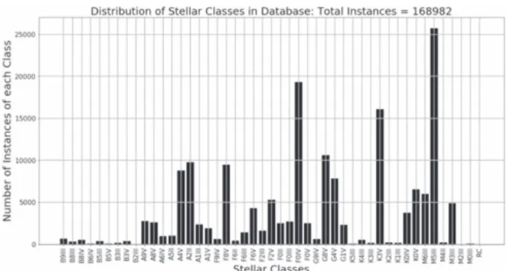
The usable data set contains 168,982 stellar spectra and 46 of the 420 class combinations. It is important to note that this is real collected data and not simulated data. The spectra arefirst preprocessed by scaling theflux to ensure that similar classes have similarflux measurements using Equation(1).

Then feature selection is performed using Algorithm 1, where the variable bounds is the number offlux measurements before and after the absorption line. The variable bounds is set to 8 to cover the RV range of−552 to 552 km s−1and ensure that sufficientflux measurements are recorded. This results in a region of 17 flux measurements around H_δ (4102Å) and a region of 17 flux measurements around the CaI (4227 Å) absorption line, which is combined to form a 34-dimension feature matrix.

After the feature selection phase, the data set is split into two subsets for RV: one for RV less than 200 km s−1and one for RV greater than 200 km s−1. Each subset is again divided into 10 subsets for tenfold cross validation (Kohavi 1995). One subset from each RV set is taken as testing sets respectively. The remaining subsets are combined into one training set. Due to the data set being imbalanced(Figure3), the training set is balanced using an undersampling method (Japkowicz 2000;

Figure 1.Example of the same spectral class with different wavelength width (FWHM)for the same absorption line for different MK classes.

Figure 2. Example of how RV is accounted for in the feature selection window.

4

Simpliﬁed BOSS spectrograph explanation:https://www.sdss.org/instruments/ boss_spectrograph/.

(5)

randomly removing samples), an oversampling method ( ran-domly duplicating samples using the synthetic minority over-sampling technique, SMOTE; Chawla et al. 2002), and a hybrid method (undersampling+oversampling). Then, KNN and RF classiﬁers are applied to the training set and tested using the RV less than 200 km s−1test set and RV greater than

200 km s−1test set as well as a combined test set. These steps are repeated 10 times with different subsets used for testing for tenfold cross validation. The accuracy, precision, recall, and F1 score(deﬁned below)are averaged over each cross validation. Misclassiﬁcation costs for incorrectly classifying a spectrum are not explored.

Table 2

Example of the Feature Matrix with Observed A0 Spectra

Star Wavelength: Wavelength: Wavelength: Wavelength: Wavelength:

Class 4101.00Å 4101.94Å 4102.89Å 4103.83Å 4104.77Å A0 L Hδ L L L A0 Hδ L L L L A0 L L Hδ L L A0 L L L Hδ L A0 L L L L Hδ

Note.Note for the A0 stars, RV causes the Hδabsorption line to be modeled with different wavelength features.

(6)

The experiments are implemented in Python, using scikit-learn (Pedregosa et al. 2011). Due to the size of the data set

(16.7 GB, which is larger than the RAM used in these experiments), the Python NumPy memmap5 (Oliphant 2015) module was used to read very large arrays from storage rather than RAM. The experiments are performed on a personal computer with the following relevant speciﬁcations: AMD Ryzen 7 1800x 16 logical core CPU, 16 GB RAM, and 1 TB Samsung 860 EVO Solid State Drive.

KNN and RF use the scikit-learn default parameters

(Pedregosa et al. 2011). Precision,6recall,7and F1 score8are computed using functions implemented by the scikit-learn sklearn.metrics package (Pedregosa et al. 2011). Feature selection is implemented using Algorithm 1 in Python and uses the Python multiprocessing package9for parallelization.

Precision is the measure of how well a predicted class compares to actual classes. (Marsland2015). For example, in the binary class case, precision is the number of samples correctly predicted as class 1 divided by the total number of samples predicted as class 1 (Equation (2)). Recall is the measure of how well an actual class compares to predicted classes(Marsland2015). For example, in the binary class case, recall is the number of samples correctly predicted as class 1 divided by the total number of samples that are actually class 1

(Equation (3)). F1 score is a type of harmonic mean that combines precision and recall into a single metric

(Equation (4); Marsland 2015). The closer precision, recall, and F1 score are to 1, the more accurate the model. In terms of this work, precision, recall, and F1 score are reported as an average of all the individual precision, recall, and F1 score measurements associated with each of the 46 classes respectively. Precision, recall, and F1 score are deﬁned in the binary class case as follows:

( ) = + Precision Total_TP Total_TP Total_FP 2 ( ) = + Recall Total_TP Total_TP Total_FN 3 ( ) = * + F 2Precision Recall Precision Recall, 4 1

where the true positive(TP)is defined as a prediction of class 1 being correctly classified as class 1, false positive (FP) is defined as a prediction of class 1 being incorrectly classified as class 2, and false negative(FN)is defined as a sample of class 1 being incorrectly predicted as class 2. In the multiclass problem, FP is defined as a prediction of class i being incorrectly classified as class¹iand FN is defined as a sample of class i being incorrectly predicted as class ¹i. More information regarding precision, recall, and F1 score can be found in Powers(2011).

4. Discussion

Tables 3 and 6 show that classification using KNN has essentially the same accuracy as RF when using hybrid and oversampling balancing. These tables demonstrate that using KNN and RF along side Algorithm 1 for feature selection are viable options for the automated classification of stellar spectra because of the high accuracy achieved. Table3 demonstrates that using three neighbors for KNN classification performs the best for KNN. Table6shows that changing the number of trees used in RF does not significantly change the classification accuracy. Tables 3 and 6 show that oversampling balancing outperforms hybrid balancing.

Table 3

Tenfold Cross-validation Accuracy for KNN

Balance Method RV Accuracy(%)for K Neighbors

3.0 5.0 7.0 10.0 15.0 20.0 Undersampled All 52.66 52.31 51.47 50.73 49.63 48.49 <200 km s−1 53.32 52.99 52.17 51.45 50.35 49.23 200 km s−1 _23.97 _22.94 _21.18 _19.38 _17.98 _16.67 Hybrid All 93.02 92.63 92.31 91.85 91.26 90.73 <200 km s−1 92.92 92.56 92.26 91.82 91.28 90.77 200 km s−1 97.15 95.62 94.44 92.94 90.54 88.96 Oversampled All 95.48 95.00 94.54 93.98 93.24 92.58 <200 km s−1 95.46 94.99 94.56 94.02 93.32 92.69 200 km s−1 96.41 95.28 93.91 92.18 89.54 87.78

Figure 3.Distribution of classes in the data set. RC=remaining classes of 0 instances.

5

Memmap: https://docs.scipy.org/doc/numpy-1.14.0/reference/generated/ numpy.memmap.html.

6 _{Precision scikit-learn:} _https:_//_{scikit-learn.org}_/_stable_/_{auto_examples}_/_{model_} selection/plot_precision_recall.html.

7

Recall scikit-learn:https://scikit-learn.org/stable/modules/generated/sklearn. metrics.recall_score.html#sklearn.metrics.recall_score.

8

F1 Score scikit-learn: https://scikit-learn.org/stable/modules/generated/ sklearn.metrics.f1_score.html#sklearn.metrics.f1_score.

9

Multiprocessing:https://docs.python.org/3.7/library/multiprocessing.html# module-multiprocessing.

(7)

Tables4and7show that the precision and recall is less than accuracy (Tables 3 and 6). The precision implies on average that the RF model’s prediction of class i is actually 84.91%

(Table 7) class i. Where recall implies on average, the RF model predicts 86.63%(Table7)of the samples that are class i as class i. It is important to note that the test sets for all RV, RV<200 km s−1, and RV 200 km s−1 metrics are tested using the same trained model. As seen in these tables, this approach accurately classiﬁes both RV<200 km s−1 and RV 200 km s−1. However, RV 200 km s−1has a higher accuracy, precision, and recall (Table 7) than RV < 200 km s−1. This could be the result of an imbalance between low RV and high RV samples and overﬁtting the model in the low RV range. Future work will attempt to increase precision and recall for low RV, which includes balancing the RV range. Tables 5 and 8 show the execution times for each experiment. These tables show that KNN performs much faster than RF. KNN has a faster train time than RF, but RF has a faster test time than KNN. For both KNN and RF, feature selection takes approximately the same amount of time, which is expected since they both use the same feature selection.

This approach takes considerably fewer steps than the one in Bolton et al. (2012) and produces excellent results. The execution times and the obtained accuracy demonstrate that, for a real application of this work, the automated classification of observed stellar spectra into a complete MK classification using a single classifier not only achieves a high accuracy but is also fast.

These experiments yielded an accuracy of 97.16% for RF

(Table6)using oversampling balancing and 150 decision trees

(Table 6), which is signiﬁcantly better than Xing & Guo

(2004), who report 81.66% accuracy for just the support vector machine (SVM) with no data reduction, 93.26% for wave-let+SVM, and 81.30% for PCA+SVM. Schierscher &

Paunzen (2011) are able to achieve an 85% match in comparison with the Sloan Extension for Galactic Under-standing and Exploration(SEGUE)Stellar Parameter Pipeline using an artiﬁcial neural network, but this is not comparable since they did not classify into direct spectral and luminosity classes. Schierscher & Paunzen(2011)also never addresses the fact that their data is imbalanced.

Other authors such as Bazarghan & Gupta(2008), Yi & Pan

(2010), and Zhang et al.(2008)do not report metrics that are comparable to the work conducted in this paper. Bazarghan & Gupta(2008)used a probabilistic neural network implemented in MATLAB and they used a χ2 value to determine classification accuracy. They make the assumption that a χ2 value of 0.002 or lower is considered classified correctly, then they achieved a success rate of about 88% in only a few seconds. Yi & Pan (2010) find that RF performed better than the MLP with an rms error (RMSE) of 1.04 and 1.36, respectively. Zhang et al. (2008) separated the classification into two classifiers. For the spectral classes, the authors used a nonparameter regression method. For the luminosity classes, the authors removed or normalized the continuum of the spectra and used a partial least-squared regression method. Zhang et al. (2008) used three spectra data sources: Silva & Cornell(1992), Pickles(1998), and Jacoby et al.(1984). They achieved a standard deviation of σ=0.7994 for the spectral classes andσ=0.58159 for the luminosity classes.

As described above in Section3, these experiments deal with data collected by a real astronomical survey. As such, when an astronomical survey points their telescopes into the sky, they get the samples (classes) that they get. The experiments presented here deal with a subset of all possible class combinations. It is important to note that not all possible class combinations(O, B, A, F, G, K, and M with subclasses of 0–9 combined with I, II, III, IV, V, VII)are common or even found in nature. Therefore, even though this approach yielded great results, there cannot be a claim that this approach will guarantee work for all stellar classes. There is, however, some theoretical validity to this approach.

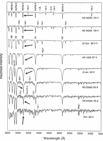
Referencing Figure3, O-type stars are the only spectral class not found in the data set. Figure4shows that O-type stars also contain the H_δabsorption line. Therefore, the missing spectral and luminosity classes are compatible with this approach because every spectral major class has at least one absorption line in the feature selection regions, which allows for the variation in width for luminosity classes.

Table 4

Tenfold Cross-validation Precision, Recall, and F1 Score for KNN Using Oversampling

RV K Neighbors 3.0 5.0 7.0 10.0 15.0 20.0 Precision All 0.805493 0.795833 0.789050 0.781626 0.767124 0.756264 <200 km s−1 0.803331 0.793968 0.787575 0.780606 0.766780 0.756458 200 km s−1 0.926071 0.897225 0.872481 0.838610 0.793230 0.756975 Recall All 0.835391 0.834499 0.834981 0.835475 0.833052 0.829150 <200 km s−1 0.832799 0.831953 0.832601 0.833312 0.831288 0.829150 200 km s−1 _0.941410 _0.921932 _0.905449 _0.879239 _0.853662 _0.959524 F1 Score All 0.811617 0.805477 0.801665 0.796227 0.786297 0.776893 <200 km s−1 0.809250 0.803309 0.799771 0.794651 0.785290 0.776297 200 km s−1 0.989692 0.985351 0.981322 0.975739 0.967290 0.827752 Table 5

Tenfold Cross-validation Execution Times for KNN Using Oversampling for all RV

Time in Seconds for K Neighbors

3.0 5.0 7.0 10.0 15.0 20.0

Feature Selection 90.89 90.89 90.89 90.89 90.89 90.89

Train 6.91 6.91 6.95 6.94 6.88 6.82

Test 3.03 3.22 3.41 3.62 3.92 4.19

(8)

5. Conclusion

The results shown in this paper support that accurate automatic stellar classiﬁcation can be obtained using astro-nomical-speciﬁc feature selection. Compared to previous work of other authors, there are four interesting conclusions. They are as follows.

1. A high level of accuracy can be obtained by considering only ﬂux measurements at wavelengths near the H_δand CaIabsorption lines.

2. A complete MK classification can be identified using a single classifier with a high level of accuracy for stars with small RV (the range of≈±240 km s−1). However, for stars with large RV (outside the range of

≈±240 km s−1), increasing the value of bounds in Algorithm 1 should compensate for large RV, but at the

cost of an increase to the computational time because of the increase in dimensions.

3. Correcting for RV is not necessary because of a sufﬁcient distribution of samples with different RV.

4. Aside from ﬂux scaling, any additional spectrum preprocessing after recombining and rebinning the spectra as presented by Dawson et al. (2013) and Stoughton et al.(2002) is unnecessary for SDSS stellar spectra.

Therefore, this new approach for the automatic classiﬁcation of stellar spectra is feasible, useful, and accurate. Future work will be conducted with the concepts of this approach to automatically classify stars and large redshift objects such as galaxies and quasars. Future work will also include building the training set with an equal distribution of RV and experiment using SMOTE or similar algorithms to build a training set

Table 6

Tenfold Cross-validation Accuracy for RF

Balance Method RV Accuracy(%)for N Trees

10.0 50.0 100.0 150.0 200.0 250.0 Undersampled All 52.45 58.13 58.75 59.01 59.09 59.21 <200 km s−1 53.09 58.78 59.39 59.65 59.72 59.83 200 km s−1 _24.62 _29.79 _30.85 _31.48 _31.77 _31.91 Hybrid All 93.83 94.44 94.48 94.48 94.50 94.49 <200 km s−1 93.73 94.35 94.38 94.39 94.41 94.41 200 km s−1 98.39 98.36 98.36 98.44 98.61 98.41 Oversampled All 96.39 97.05 97.12 97.16 97.15 97.16 <200 km s−1 96.34 97.01 97.09 97.13 97.12 97.12 200 km s−1 98.49 98.65 98.62 98.62 98.65 98.65 Table 7

Tenfold Cross-validation Precision, Recall, and F1 Score for RF Using Oversampling

RV N Trees 10.0 50.0 100.0 150.0 200.0 250.0 Precision All 0.827606 0.845460 0.849466 0.849149 0.850188 0.850051 <200 km s−1 0.825895 0.844077 0.848296 0.847941 0.848908 0.848765 200 km s−1 0.968922 0.971134 0.967166 0.968655 0.971852 0.971852 Recall All 0.849646 0.862420 0.866250 0.866379 0.868213 0.868580 <200 km s−1 0.847837 0.861001 0.865014 0.865182 0.866917 0.867305 200 km s−1 0.973081 0.973082 0.970220 0.972075 0.972433 0.972433 F1 Score All 0.832101 0.847679 0.851134 0.851346 0.852966 0.853006 <200 km s−1 0.830256 0.846204 0.849857 0.850088 0.851616 0.851663 200 km s−1 0.969936 0.970727 0.967720 0.969363 0.970591 0.970591 Table 8

Tenfold Cross-validation Execution Times for RF Using Oversampling for All RV Time in Seconds for N Trees

10.0 50.0 100.0 150.0 200.0 250.0

Feature Selection 90.89 90.89 90.89 90.89 90.89 90.89

Train 129.23 605.32 1226.75 1857.21 2448.32 2960.94

(9)

using a small number of real samples to simulate how this approach could work for a new spectroscopic survey.

ORCID iDs

Michael J. Brice https://orcid.org/0000-0002-1278-2404 References

Bai, Y., Liu, J., Wang, S., & Yang, F. 2019,AJ,157, 9

Bailer-Jones, C. A. L., Irwin, M., & von Hippel, T. 1998,MNRAS,298, 361

Bazarghan, M. 2008, arXiv:0804.2742

Bazarghan, M., & Gupta, R. 2008,Ap&SS,315, 201

Bolón-Canedo, V., Sánchez-Maroño, N., & Alonso-Betanzos, A. 2015, Feature Selection for High-Dimensional Data(Cham: Springer)

Bolton, A. S., et al. 2012,AJ,144, 144

Breiman, L. 2001,Machine Learning, 45, 5

Brice, M., & Andonie, R. 2019, in Proc. Int. Joint Conf. Neural Networks (INNS) (Piscataway, NJ: IEEE), 1

Chawla, N. V., Bowyer, K. W., Hall, L. O., & Kegelmeyer, W. P. 2002,JAIR, 16, 321

Dawson, K. S., et al. 2013,AJ,145, 10

Duan, F.-Q., Liu, R., Guo, P., Zhou, M.-Q., & Wu, F.-C. 2009, RAA,9, 341

Elting, C., Bailer-Jones, C. A. L., & Smith, K. W. 2008, in AIP Conf. Proc. 1082, Classiﬁcation and Discovery in Large Astronomical Surveys, ed. C. A. I. Bailer‐Jones(Melville, NY: AIP),9

Goldberger, J., Hinton, G. E., Roweis, S. T., & Salakhutdinov, R. R. 2005, in Advances in Neural Information Processing Systems 17, ed. L. K. Saul, Y. Weiss, & L. Bottou(Cambridge, MA: MIT Press), 513

Gray, R. O., & Corbally, J. C. 2009, Stellar Spectral Classiﬁcation(Princeton, NJ: Princeton Univ. Press)

Ivezic, Z., Connolly, A., VanderPlas, J., & Gray, A. 2014, Statistics, Data Mining, and Machine Learning in Astronomy: A Practice Python Guide for the Analysis of Survey Data(Princeton, NJ: Princeton Univ. Press) Jacoby, G. H., Hunter, D. A., & Christian, C. A. 1984,ApJS,56, 257

Japkowicz, N. 2000, Learning from Imbalanced Data Sets, Tech. Rep. WS-00-05

Kohavi, R., & Li, C.-H. 1995, in Proc. 14th Int. Joint Conf. Artiﬁcial Intelligence, Vol. 2, IJCAI’95 (San Francisco, CA: Morgan Kaufmann Publishers Inc), 1137

Marsland, S. 2015, Machine Learning: An Algorithmic Perspective(2nd ed.; Boca Raton, FL: CRC Press)

Morgan, W. W., Keenan, P. C., & Kellman, E. 1943, An Atlas of Stellar Spectra, with an Outline of Spectral Classiﬁcation (Chicago, IL: Univ. Chicago Press)

Oliphant, T. E. 2015, A Guide to NumPy (Spanish Fork, UT: Trelgol Publishing)

Pedregosa, F., Varoquaux, G., Gramfort, A., et al. 2011, J. Mach. Learn. Res., 12, 2825

Pickles, A. J. 1998,PASP,110, 863

Powers, D. 2011,J. Mach. Learn. Technol, 2, 37 Sánchez, A. J., & Prieto, C. A. 2013,ApJ,763, 50

Schierscher, F., & Paunzen, E. 2011,AN,332, 597

Shlens, J. 2014, arXiv:1404.1100

Silva, D. R., & Cornell, M. E. 1992,ApJS,81, 865

Smee, S. A., Gunn, J. E., Uomoto, A., et al. 2013,AJ,146, 32

Stoughton, C., Lupton, R. H., Bernardi, M., et al. 2002,AJ,123, 485

Xing, F., & Guo, P. 2004, in Advances in Neural Networks, ed. F.-L. Yin, J. Wang, & C. Guo(Berlin: Springer), 616

Yi, Z., & Pan, J. 2010, Inter. Congress on Image and Signal Processing (Piscataway, NJ: IEEE), 3129

York, D. G., et al. 2000,AJ,120, 1579

Zhang, J. N., Luo, A. L., & Tu, L. P. 2008, in Inter. Congress on Image and Signal Processing(Piscataway, NJ: IEEE), 249

Figure 4. Sample of continuum normalized spectra from O—G type stars (Gray & Corbally2009). The arrows point to the Hδabsorption line.