Forecasting energy data with a time lag into the future and Google trends

Cit a ti o n

H a s s a n i, H . a n d Silv a, E. S. ( 2 0 1 6 ) F o r e c a s ti n g e n e r g y d a t a

wi t h a ti m e l a g i n t o t h e f u t u r e a n d Go o gl e t r e n d s .

I n t e r n a ti o n al Jo u r n al of E n e r g y a n d S t a ti s ti c s , 4 ( 4). p p .

1 6 5 0 0 2 0-1 .

C r e a t o r s

H a s s a n i, H . a n d Silv a, E. S.

U s a g e G u i d e l i n e s

Pl e a s e r ef e r t o u s a g e g u i d eli n e s a t

h t t p :// u al r e s e a r c h o n li n e . a r t s . a c . u k / p olici e s . h t m l

o r a l t e r n a tiv ely c o n t a c t

u a l r e s e a r c h o n li n e @ a r t s . a c . u k

.

Vol. 4, No. 4 (2016) 1650020 (11pages) c

Institute for International Energy Studies DOI:10.1142/S2335680416500204

Forecasting energy data with a time lag into the future and Google trends

Hossein Hassani∗,‡and Emmanuel Sirimal Silva†,§

∗_{Institute for International Energy Studies}

Tehran, Iran

†_{Fashion Business School, London College}

of Fashion, University of the Arts London, UK

‡_{[email protected]} §_{[email protected]} Received 22 October 2016 Revised 25 November 2016 Accepted 27 November 2016 Published 31 December 2016

This paper presents a new idea for a forecasting approach which seeks to exploit the information contained within US EIA energy forecasts and related Google trends data for generating a new and improved forecast. The novel forecasting approach can be exploited by using a multivariate system which can consider data with different series lengths and a time lag into the future. Using real historical data, an official forecast for the same variable, and Google Trends search data, we illustrate the possibility of generating a comparatively more accurate forecast for an energy-related variable. The accuracy of the newly generated forecasts are evaluated by comparing with the actual observations and the official forecast itself. We find that the novel forecasting idea can generate promising results which call for further in-depth research into developing and improving this multivariate forecasting approach.

Keywords: Forecastability; energy forecasts; official forecasts; Google trends; future time lagged data.

Nomenclature

EIA: Energy Information Administration.

ST EO: Short Term Energy Outlook.

MSSA: Multivariate Singular Spectrum Analysis.

SV D: Singular Value Decomposition.

L: Window Length.

LRF : Linear Recurrent Formula.

US: United States.

RMSE: Root Mean Square Error.

RRMSE: Ratio of the RMSE.

DC : Direction of Change.

1. Introduction

Forecasting is an art which continues to be of primary importance for resource allocation and planning within the global energy sector. The importance of energy forecasts for planning and resource allocations are clearly evident in the variety of energy-related forecasts which are published by the US EIA via their STEO reports [1]. Whilst the practice of publishing monthly energy-related forecasts have been in existence over a long period, more recently, Google provided users with access to real-time data on online search queries in the form of Google Trends.a Google Trends are often found to be correlated with economic indicators and may be useful for short term economic prediction [2]. Moreover, Google Trends are rec-ognized as excellent indicators of public concern and has the potential of being a useful quantitative measure of energy related events [3]. It is noteworthy that the emergence of Big Data such as Google Trends has resulted in an increased avail-ability of real-time information which can be extremely useful for improving the accuracy of forecasts [4].

This paper looks at exploiting both the availability of forecasts for energy-related variables and the access to Google Trends data as we introduce a new forecasting approach within the broad field of time series analysis and forecasting. Accordingly, there are several key contributions which are noteworthy. First, the new multivariate forecasting approach that is introduced herewith is different to the forecast averaging and forecast combination approaches in time series. This is because here we seek to model and extract information from data with a time lag into the future. Second, the approach itself can be exploited by any multivariate forecasting technique which can model data; with different series lengths and a time lag into the future. Third, to the best of our knowledge the application which follows presents the results from the initial attempt at using the chosen multivariate forecasting tool in combination with Google Trends.

Energy-related data are usually affected by many factors including demand, sup-ply, economics, policy, technology, and weather, in addition to noise levels, volatility and nonlinear patterns. Therefore, we have opted for a nonparametric multivari-ate signal processing technique that can capture the nonlinear pattern of noisy volatile data with different series lengths as the tool for forecasting with forecasts and Google Trends. The chosen multivariate forecasting technique is complemented with auxiliary information in the form of official forecasts (which effectively repre-sents data with a time lag into the future) and Google Trends. The accuracy of the

forecast achieved via the newly proposed approach is evaluated by comparing with actual data and the official forecast over the same period.

It should be noted that is not our intention or aim to claim that Google Trends can predict the future, and we subscribe to the views expressed in [2] where the authors suggest that Google Trends are more useful for contemporaneous forecast-ing or nowcastforecast-ing. However, here we simply seek to present a new idea which can show the benefits of incorporating Google Trends in a multivariate process which considers data with a time lag into the future. Even though we consider an energy-related data set as an example, it is not our intention to indicate that we can forecast tomorrow’s energy price. Instead, we seek to introduce this new concept for improving the accuracy of forecasts by exploiting the forecastability of official forecasts, and show that the inclusion of Google Trends data within such a frame-work can result in a forecast that is more accurate than an existing official forecast. The addition of more related information into the multivariate system can help improve the forecast further.

The remainder of this paper is organized such that Sec.2 presents a summary of the proposed forecasting approach which is followed by an introduction to the data, metrics, and results following application in Sec. 3. The paper concludes in Sec.4.

2. Forecasting with Official Forecasts and Google Trends

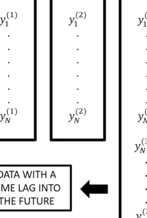
Let us begin by inputting data into the multivariate system as shown via Fig.1. Here, the observations represented via (y₁(1), . . . , y_N(1)) ≡ (y(3)₁ , . . . , y(3)_N ) as these represent the historical data for the variable of interest. Then, the observations within (y(3)_N+1, . . . , y(3)_N+h) represents the official forecast and thus data which has a time lag into the future. The observations in (y(2)₁ , . . . , y_N(2)) in this example will represent data from Google Trends, but in general it could represent any auxiliary information and the multivariate system can incorporate additional variables in the modelling process.

In what follows, we seek to summarize the entire forecasting with official fore-casts and Google Trends process concisely via the following steps.

(1) Consider three time seriesY_N(1),Y_N(2)andY_N(3)_+hsuch thatY_N(1)= (y₁(1), . . . , y(1)_N ),

Y(2)

N = (y(2)1 , . . . , yN(2)), and YN(3)+h = (y (3)

1 , . . . , yN(3)+h) with an identical

fre-quency. Here,Y_N(1) andY_N(2)represents historical data for a variable of interest and Google Trends data respectively.

Note:Y_N(3)_+hrepresentsY_N(1)plus theh-step ahead official forecast for that same variable. Theh-step ahead official forecast represents data with a time lag into the future.

(2) Call upon a multivariate system which can consider data with different series lengths and a time lag into the future, for forecasting with official forecasts and

Fig. 1. A graphical illustration of the data input into the system.

Google Trends. Our aim is to obtain a multivariateh-step ahead forecast for

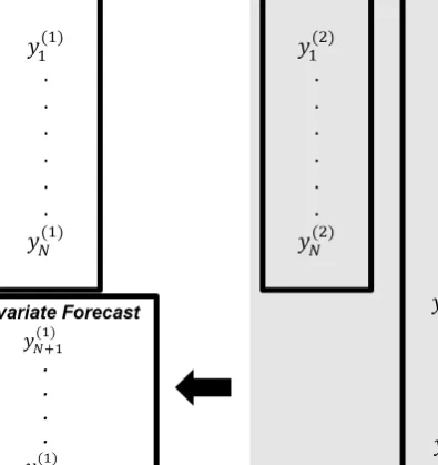
Y(1) N = (y(1)1 , . . . , y (1) N ) as represented by ˆyN(1)+1, . . . ,yˆ (1) N+hin Fig. 2.

(3) Exploit a multivariate system’s filtering and signal extraction capabilities for modelling and extracting information in Y_N(3)_+h (which represents data with a time lag into the future) andY_N(2), for generating a new and improved forecast for the variable inY_N(1). Figure2 summarises the process in graphical format. (4) In this paper we exploit Multivariate Singular Spectrum Analysis (MSSA) as

the multivariate system. Those interested in a detailed description of the theory underlying this nonparametric technique are referred to [5]. However, below we provide a very brief introduction into the MSSA process.

The MSSA technique consists of two stages known as decomposition and recon-struction. The decomposition stage has two steps known as embedding and SVD. Initially, through embedding we create the trajectory matricesX(i)_{(i= 1,2,3) of}

the one-dimensional time seriesY_N(1),Y_N(2) andY_N(3)_+hrespectively. Accordingly, we will have 3 differentL_i×K_i trajectory matricesX(i)_{(i= 1,2,3), whereX}(1) _will

Fig. 2. A graphical illustration of the process and objective.

take the form:

X(1)= (x_ij)L,K_i,j=1=        y1 y2 · · · yK y2 y3 · · · yK+1 .. . ... . .. ... yL yL+1 · · · yN        . (1)

A similar trajectory matrix as in Eq. (1) can be constructed for X(2) to represent the data inY_N(2). Finally, the trajectory matrixX(3) _{which incorporates the official}

forecast can be constructed as:

X(3)= (x_ij)L,K_i,j=1+h=        y1 y2 · · · yK yK+1 · · · ωK+h y2 y3 · · · yK+1 yK+2 · · · ωK+h+1 .. . ... . .. ... ... . .. ... yL yL+1 · · · yN ωN+1 · · · ωN+h        , (2)

Thereafter, a new block Hankel trajectory matrix,X_H is constructed. Assume

L1 =L2 = · · · = L_M =L where M is the number of time series. Therefore, we have different values ofK_i(K_i =N_i−L_i+ 1) and series lengthN_i, but similarL_i. The result of this step is:

X_H= [X(1) :X(2):· · ·:X(M)]. Hence, the structure of the matrixX_HXT_H is as follows:

X_HXT_H=X(1)X(1)T +· · ·+X(M)X(M)T. (3) As it appears from the structure of the matrix X_HXT_H in MSSA, we do not have any cross-product between Hankel matrices X(i) _{and X}(j)_{. Moreover, in this}

format, the sum ofX(i)X(i)T provides the new block Hankel matrix. Note also that performing the SVD ofX_H in MSSA yieldsLeigenvalues as in univariate SSA.

Thereafter, in the reconstruction stage we are faced with two steps known as grouping and diagonal averaging. Initially, we group the eigenvalues from the SVD process as either signal or noise (there are several approaches for grouping, see [5,6]) and then perform diagonal averaging on the signal components to reconstruct a new, less noisy time series which can be used for forecasting. A more detailed description of the theory underlying decomposition and reconstruction with MSSA and the forecasting process can be found in [5] and is therefore not reproduced here.

Finally, we present the MSSA forecasting algorithm used in this paper, and in doing so we mainly follow [5].

(1) For a fixed value ofL, construct the trajectory matrixX(i)= [X₁(i), . . . , X_K(i)] = (x_mn)L,Ki

m,n=1 for each single seriesYN(ii)(i= 1, . . . , M) separately. (2) Construct the block trajectory matrixX_H as follows:

X_H = [X(1):X(2):· · ·:X(M)].

(3) Let vector U_Hj = (u1_j, . . . , u_Lj)T, with length L, be the jth eigenvector of

X_HXT_H.

(4) ConsiderX_H =r_i=1U_HiU_HT

iXH as the reconstructed matrix obtained using

reigentriples:

X_H =X(1):X(2):· · ·:X(M)].

(5) Consider matrixX(i)=HX(i)(i= 1, . . . , M) as the result of the Hankelization procedure of the matrixX(i) _{obtained from the previous step.}

(6) LetU_H

j denote the vector of the firstL−1 coordinates of the eigenvectorsUHj, andπ_Hj indicate the last coordinate of the eigenvectorsU_Hj (j= 1, . . . , r).

(7) Defineυ2₌r

j=1πH2j.

(8) Denote the linear coefficients vectorRas follows:

R= 1 1−υ2 r j=1 πHjUHj . (4)

(9) Ifυ2_{<1, then theh-step ahead MSSA forecasts exist and is calculated by the} following formula: ˆ y(1) j1 , . . . ,yˆ (M) jM T = [˜y_j(1) 1 , . . . ,y˜ (M) jM ], ji= 1, . . . , Ni, RT_{Zh, ji=Ni+ 1, . . . , Ni+h,} (5) where, Z_h = [Z_h(1), . . . , Z_h(M)]T and Z_h(i) = [ˆy(_Ni) i−L+h+1, . . . ,yˆ (i) Ni+h−1] (i = 1, . . . , M).

Note that Eq. (5) indicates that the h-step ahead forecasts of each series are achieved by the same LRF generated considering all series in a multivariate system.

3. Data, Metrics and Application 3.1. Data

This paper considers historical monthly data from January 2011–November 2015 as in-sample for model training and testing whilst the forecasting performance is eval-uated over the period from December 2015–November 2016 (12 observations) such that it is a one-year ahead forecast. The variable being forecasted is the Henry Hub Spot price for Natural Gas (dollars per million Btu). The official monthly forecasts for the Henry Hub Spot price between December 2015–November 2016 as provided via the US EIA, and monthly Google Trends data for the search term ‘Natural Gas Price’ (January 2011–November 2015) are used as auxiliary information. The actual values corresponding to the EIA forecasts considered in this paper have been published in the December 2016 STEO report [1].

3.2. Metrics

3.2.1. RMSE and RRMSE

We rely on the RMSE and RRMSE criterions for evaluating forecast accuracy. Both these criterions are popular and frequently cited loss functions, see for example [8,9].

RMSE = 1 n n i=1 (Y_i−Yˆ_i)2 1 2 , (6)

where,Y_iis the actual value, ˆY_irefers to a forecast from a given model, andnis the number of the forecasts. Likewise, the ratio of the RMSE can be easily calculated as:

RRMSE = RMSEProposed Approach

RMSE_Benchmark , (7)

where RMSE_{Proposed Approach} refers to the RMSE from the proposed multivariate system and RMSE_Benchmark refers to the RMSE for the official forecast. Then, if the RRMSE is less than 1 the proposed multivariate approach outperforms the benchmark model by 1-RRMSE%.

3.2.2. Direction of change probability

The application which follows considers a forecast for the gas price. When predicting such variables it is important that forecasts are not only able to report a low error as measured by the RMSE, but also successful in capturing or predicting the actual direction of change and movement in future prices. As such, we consider the DC criterion as a metric (see, [10,11] for examples of previous applications) and present its calculation by following [10]. Let Z_Yi take the value 1 if the forecast correctly predicts the direction of change and 0 otherwise. Then ¯Z_Y =n_i=1Z_{Y i}/nshows the proportion of forecasts that correctly predict the direction of the series. For example, if DC is 0.70 this implies that 70% of the actual movement has been captured by the forecasting method.

3.3. Application

Let us now consider the performance of the proposed multivariate system at fore-casting 12-months ahead for the Henry Hub Spot price, for which the results are reported in Table 1. All forecasts have been evaluated for statistically significant differences between competing forecasts via the HS test in [7]. We begin by focus-ing on the RMSE criterion. The first observation is that the MSSA models can provide forecasts with a lower RMSE than the EIA official forecast for the same variable. This implies that the proposed forecasting with official forecasts approach (MSSA|(EIA)) works in practice and can provide useful forecasting accuracy gains. In fact, by using only the official forecast provided by EIA as auxiliary information, we are able to generate a new forecast which is 6% more accurate than the EIA official forecast (as measured by the RRMSE: 1−0₀._.51₅₄. Therefore, we can conclude that considering future information as auxiliary information aids in obtaining a better forecast. Moreover, it appears that data with a time lag into the future can help to capture the general pattern of a future forecast when combined with past data.

Next, let us consider using both the EIA forecast and Google Trends data as auxiliary information. Based on the RMSE values it is clear that MSSA|(EIA,GT) is able to outperform the EIA and MSSA|(EIA) forecasts for the Henry Hub Spot price. This in turn implies that the incorporation of Google Trends within the

Table 1. Henry Hub Spot forecasting RMSE and RRMSE results.

RMSE RRMSE

Series EIA MSSA|(EIA) MSSA|(EIA,GT) MSSA_EIA|(EIA,GT) MSSA_MSSA|(EIA_|(EIA),GT)

Henry Hub Spot 0.54 0.51 0.45 0.83 0.88

Note: MSSA|(EIA) represents the MSSA results with only the official forecast as auxiliary infor-mation. MSSA|(EIA,GT) represents the MSSA results with both the official forecast and Google Trends as auxiliary information.

Table 2. Direction of change results for Henry Hub Spot forecasts.

Series EIA MSSA|(EIA)

Henry Hub Spot 0.58 0.75

Note: MSSA|(EIA) represents the MSSA model with only the official forecast as auxiliary information.

newly proposed forecasting with official forecasts framework can result in positive

outcomes in terms of improved accuracy levels. As the MSSA|(EIA,GT) model

reports the lowest RMSE, we consider this as the numerator in calculating the RRMSE values which are also reported via the last two columns in Table1. Accord-ingly, we can see that the inclusion of GT within our framework has enabled us to produce a forecast which is 17% more accurate than the EIA official forecast.

The MSSA|(EIA,GT) forecast is also 12% more accurate than the MSSA|(EIA)

forecast. Our findings are in line with previous research which also indicated that Google Trends can help with improving energy market analysis [3,12]. However, in this case we do not find any evidence of statistically significant differences between the MSSA|(EIA,GT) forecasts and competing forecasts, and this can be attributed to the low sample size of 12 observations.

Finally, let us now consider how well the official forecast and MSSA|(EIA) forecast perform in terms of capturing the movement in future prices by looking at the direction of change results. These are reported in Table2. We find that the EIA official forecast reports a 58% accurate DC prediction. However, the MSSA|(EIA) forecast reports a DC prediction at 75% which is a 17% gain in relation to the official forecast. This clearly indicates yet another advantage in being able to exploit data with a time lag into the future as it enables the capturing of dynamic price changes which are likely to happen in future. Accordingly, these results show that the MSSA|(EIA) forecasts are more likely to accurately capture the movements in gas prices in comparison to the official forecast.

4. Conclusion

This paper presents a new idea for forecasting with official forecasts and improving accuracy levels further via the incorporation of auxiliary information in the form of Google Trends data. The aim being, to use the new forecasting idea to generate a forecast that can outperform the accuracy of the official forecast. The process is unique as it involves the modelling of data with a time lag into the future, which requires a multivariate system that can model data with different series lengths. The general idea is concisely presented to the reader in the most basic form, clearly outlining the nature of the suggested process. Thereafter, the proposed idea is put into action by applying the concept to real world data from the US EIA. We find promising results which not only show the applicability of the newly proposed

forecasting idea in practice, but also shows the positive influence of Google Trends on improving forecast accuracy.

Here we consider monthly data and a single energy variable as an example. How-ever, the proposed forecasting idea is applicable to data from any given frequency and can be applied to forecast any given energy variable. Moreover, the idea itself can be exploited by any multivariate forecasting technique which can model data with different series lengths and a time lag into the future, even though we con-sider MSSA as a tool in this paper. In addition, it should be noted that users are not restricted to exploiting official forecasts. It is possible to consider and exploit information from forecasts generated via other time series models or professional forecasts as well.

We believe that the favourable results presented here open up a new research avenue in the field of time series analysis and forecasting. Future research should consider developing a more theoretically sound methodology for the proposed fore-casting approach, optimization criteria for the tools used, and perform tests on a variety of different data sets. In terms of selecting the most appropriate search terms for matching with a variable of interest, researchers could consider Google Correlate [13] which can identify search patterns which correspond with real-world trends. Finally, there is huge scope and potential to incorporate Big Data within the proposed framework for forecasting with official forecasts and Google Trends — the possibilities are endless as there is no restriction on the number of variables one could input into the multivariate system.

References

[1] STEO Archives (2016). Available via: http://www.eia.gov/outlooks/steo/outlook. cfm. [Accessed: 24.11.2016].

[2] Choi, H. and Vairan, H. (2012). Predicting the Present with Google Trends.Economic Records,88(s1), 2–9.

[3] Ji, Q. and Guo, J.-F. (2015). Oil price volatility and oil-related events: An Internet concern study perspective.Applied Energy,137, 256–264.

[4] Hassani, H. and Silva, E. S. (2015). Forecasting with big data: A review.Annals of Data Sciencie,2(1), 5–19.

[5] Sanei, S. and Hassani, H. (2015).Singular Spectrum Analysis of Biomedical Signals. CRC Press.

[6] Hassani, H., Ghodsi, Z. and Silva, E. S. (2016). From nature to maths: Improving forecasting performance in subspace-based methods using genetics Colonial Theory. Digital Signal Processing,51, 101–109.

[7] Hassani, H. and Silva, E. S. (2015). A Kolmogorov-Smirnov based test for comparing the predictive accuracy of two sets of forecasts.Econometrics,3(3), 590–609. [8] Silva, E. S. and Hassani, H. (2015). On the use of Singular Spectrum Analysis for

forecasting U.S. trade before, during and after the 2008 recession.International Eco-nomics,141, 34–49.

[9] Altavilla, C. and De Grauwe, P. (2010). Forecasting and combining competing models of exchange rate determination.Applied Economics,42(27), 3455–3480.

[10] Hassani, H., Heravi, S. and Zhigljavsky, A. (2013). Forecasting UK industrial pro-duction with multivariate Singular Spectrum Analysis.Journal of Forecasting,32(5), 395–408.

[11] Hassani, H., Webster, A., Silva, E. S. and Heravi, S. (2015). Forecasting U.S. Tourist arrivals using optimal Singular Spectrum Analysis. Tourism Management,46, 322– 335.

[12] Li, X., Ma, J., Wang, S. and Zhang, X. (2015). How does Google search affect trader positions and crude oil prices?Economic Modelling,49, 162–171.

[13] Google Correlate. (2011). Available via: https://www.google.com/trends/correlate. [Accessed: 24.11.2016].