Time series forecasting based on classification of dynamic patterns

(1)

IMT Institute for Advanced Studies, Lucca

Lucca, Italy

Time Series Forecasting Based on Classification

of Dynamic Patterns

PhD Program in Computer Science and Engineering

XXVII Cycle

By

Rodrigo L ´opez Far´ıas

2015

(2)

(3)

The dissertation of Rodrigo L ´opez Far´ıas is approved.

Program Coordinator: Prof. Alberto Bemporad, Institute of Advanced Studies Lucca

Supervisor: Dr. Alberto Bemporad, Institute of Advanced Studies Lucca

Supervisor: Dr. Pantelis Sopasakis, Institute of Advanced Studies Lucca

Tutor: Dr. Alberto Bemporad, Institute of Advanced Studies Lucca

The dissertation of Rodrigo L ´opez Far´ıas has been reviewed by:

Dr. Carlos Ocampo Mart´ınez, Universitat Polit`ecnica de Catalunya

Dr. Andrea Emilio Rizzoli, Istituto Dalle Molle di Studi sull’Intelligenza Artificiale

IMT Institute for Advanced Studies, Lucca

2015

(4)

(5)

(6)

(7)

Abstract xviii 1 Introduction 1 1.1 Problem Definition . . . 2 1.2 Main Objective . . . 4 1.2.1 Particular Objectives . . . 5 1.3 Justification . . . 5 1.4 Thesis Organisation . . . 7 2 Related Work 8 3 Time Series Forecasting and System Identification 17 3.1 Linear Time Series Analysis . . . 23

3.1.1 Decomposition Methodology in Classical Analysis 28 3.1.2 Stationarity and Sampling . . . 30

3.1.3 Testing for Stationarity . . . 31

3.1.4 Linear Autocorrelations . . . 34

3.2 Box-Jenkins Auto-Regressive Forecasting . . . 36

(8)

3.2.2 Moving-Average (MA) Models . . . 38

3.2.3 ARIMA(p,d,q) . . . 38

3.2.4 Seasonal ARIMA . . . 39

3.3 Holt-Winters: Exponential Smoothing . . . 40

3.3.1 Single Exponential Smoothing . . . 40

3.3.2 Double Exponential Smoothing . . . 41

3.3.3 Seasonal Holt-Winters . . . 43

3.3.4 Double Seasonal Holt-Winters . . . 44

3.4 k-Nearest Neighbours Forecasting . . . 45

3.4.1 Real Numbers Forecasting . . . 46

3.4.2 Qualitative Forecasting . . . 47

3.4.3 Simple Nonlinear Filter . . . 48

3.5 Radial Basis Function Artificial Neural Networks . . . 49

3.6 Error Measurement Indicators . . . 50

3.7 Classification and Clustering . . . 52

3.7.1 k-Means Clustering . . . 53

3.7.2 Selecting the Best Cluster Partition . . . 53

3.7.3 Feature Extraction . . . 56

4 Multi-Model Forecasting 59 4.1 General Predictor Architecture . . . 61

4.2 Multi-Model Forecasting Using RBF-ANN with an On-line Mode Recognition . . . 62

4.2.1 Discrete Derivative as a Feature Extraction Method 64 4.2.2 On-line Mode Recognition for the Multi-Model Pre-dictor Approach . . . 65

4.3 Multi-Model Predictor Based on Qualitative and Quanti-tative Decomposition . . . 69

4.3.1 Multi-Model Predictor Based on the Qualitative and Quantitative Decomposition of Time Series using SARIMA and kNN . . . 71

4.3.2 Multi-Model Predictor Based on the Qualitative and Quantitative Decomposition of Time Series Using SARIMA and Noise Filter . . . 73

(9)

5 Results 79

5.1 Description of the Database . . . 79 5.2 Experiments . . . 84

5.2.1 Validation and Performance Comparison ofQMMP

Algorithms . . . 85 5.2.2 Validation and Performance of the Multi-Model

Fo-recasting Using RBF Artificial Neural Networks with an On-line Mode Recognition . . . 95 5.2.3 Discussion . . . 100 6 Conclusions 102 6.1 General Conclusions . . . 102 6.2 Particular Conclusions . . . 103 6.3 Future Work . . . 105 A List of Symbols 109 Bibliography 113

(10)

List of Figures

1 Rising, oscillating, and falling patterns classification . . . . 10

2 Class 1 descriptor associated with weekend and holiday consumption patterns. ( c2014, IEEE). . . 11

3 Class 2 descriptor associated with weekdays consumption pattern. ( c2014, IEEE). . . 11

4 Phase space representation and clustered in regions of the hourly global horizontal solar radiation0_{. . . .} ₁₂

5 Measured hourly global horizontal solar radiation time se-ries of July 19960_{. . . .} ₁₃

6 Example of an application of ensemble forecasting applied to the prediction of hurricane trajectories. . . 15

7 In a finite state machine transition states are triggered by events. . . 22

8 In Markov Model transition states are triggered with cer-tain probability. . . 22

9 Secular trend . . . 24

10 Seasonal variation . . . 25

11 Noise . . . 25

12 Transient variation . . . 26

13 Additive composition example . . . 27

14 Multiplicative composition example . . . 27

15 Pseudo-additive time series example . . . 28

(11)

17 Four complete patterns . . . 32

18 General structure of the Multi-Model Predictor . . . 62

19 Multi-Model training process . . . 63

20 Time Series processing data . . . 66

21 Multi-model training process . . . 71

22 Prediction sample . . . 74

23 Multi-Model Predictor with the Filter Module . . . 75

24 Raw time series generated by different flowmeters during the year 2012. . . 81

25 Raw time series generated by different flowmeters during the year 2012 . . . 82

26 Linear regression for illustrating the trend of the selected time series . . . 83

27 Linear regression for illustrating the trend of the selected time series . . . 84

28 Autocorrelation plots of different sectors . . . 85

29 Autocorrelation plot of sector p10025 . . . 85

30 Organisation of the training-validation and test sets . . . . 86

31 Mean silhouette coefficient values for different values of k in k-means and different time series of water demand. . . . 87

32 The two pattern modes of different sectors. The week starts on Sunday. . . 87

33 Training and testing data organisation . . . 90

34 Error along the testing set of Sector 5 . . . 93

35 Prediction sample of 2 days ahead of Sector 5 . . . 93

(12)

48 Mean silhouette coefficient values for different values of k in k-means and different time series of water demand. . . . 96

49 Prediction sample Sector 5 . . . 99

56 Mean silhouette value for varying values ofkand variable prediction horizonh . . . 100

(13)

List of Tables

1 Classification of the dynamical systems according to their number of variables . . . 21 2 Number of outliers detected by the modified Thompson

tautechnique with a significance ofα= 0.01 . . . 83 3 Trend described by the slope and intercept components of

linear regression . . . 84 4 Two iteration cross validation for kNN and Calendar mode

estimation . . . 88 5 mparameters that optimize the mode prediction with kNN.

ε= 0.01was chosen for all time series . . . 89 6 Parameters for the Noise Filter, kNN Qualitative Forecaster

and SARIMA models for each time series found. . . 91 7 RM SE24performance comparison of the different

algorit-hms . . . 91 8 RM SE24indicator for each time series produced byQMMP,

DSHW,RBFMMP+ORandRBF-ANN . . . 97 9 RM SEhindicator for each method for the hourly time

(14)

Acknowledgements

I would like to thank my Advisor Dr. Alberto Bemporad, and co-advisor Dr. Pantelis Sopasakis, for their insightful com-ments and guidance for the thesis dissertation.

Thanks to IMT Institute for Advanced Studies for giving me the great opportunity and resources to finish this PhD. My sincere gratitude to my external research activity advisor Dr. Vicenc¸ Puig for his continuous support, contribution and close collaboration for this PhD thesis and the facilities pro-vided by theUniversitat Polit`ecnica de Catalunya.

Thanks to Dr. Juan J. Flores fromUniversidad Michoacana de San Nicol´as de Hidalgofor his scientific support and contribu-tion to this thesis and the invitacontribu-tion to collaborate during the final period of my PhD. Thanks also to the Electrical Engi-neering Faculty from the same University for providing me the facilities required to finish this important project.

Thanks to my friend and colleague Dr. H´ector Rodr´ıguez Rangel for his participation, support and contribution. Thanks to Dr. Carlos Ocampo M. fromUniversitat Polit`ecnica de Catalunya and Dr. Andrea E. Rizzoli from Istituto Dalle Molle di Studi sull’Intelligenza Artificialefor the useful and care-ful revision of this thesis.

Also thanks to Elseiver and IEEE for granting permission for including some material from their sources contained in Jour-nal Energy Conversion and Conference proceeding Manage-ment, Control and Automation (MED).

Thanks to my parents Lucrecia and Victor for their uncondi-tional support and patience. Now we know that great deci-sions are not usually easy to take.

(15)

Vita

July 8, 1984 Born, M´exico D.F., M´exico

2008 B. Eng. Computational Systems Final mark: 86/100

Instituto Tecnol ´ogico de Morelia, M´exico

2010 MSc. in Electrical Engineering Final mark: 93/100

Posgrado de Ingenier´ıa El´ectrica de la Universidad Mi-choacana de San Nicols de Hidalgos M´exico

(16)

Publications

1. R. Lopez, V. Puig, H. Rodriguez, “An implementation of a multi-model predictor based on the qualitative and quantitative decomposition of the time-series”, inInternational work-conference on Time Series 1. Granada, Spain, 2015.

2. R. Lopez, V. Puig, “A Multiple-Model Predictor Approach Based on an On-Line Mode Recognition with Application to Water Demand Forecasting” inInternational work-conference on Time Series 1. Granada, Spain, 2015. 3. R. Lopez, J. Flores and V. Puig, “Multi-Model Forecasting Based in a

Quali-tative and QuantiQuali-tative Decomposition with Nonlinear Noise Filter and an Application To Water Demand” in2015 IEEE International Autumn Meeting on Power, Electronics and Computing (ROPEC). Ixtapa, Mexico, 2015. 4. J. Flores, J. Ortiz Bejar, J. Rafael Cede ˜no, C. Lara-Alvarez and R. Lopez,

“FNN a Fuzzy Version of the Nearest Neighbor Time Series Forecasting Technique” in2015 IEEE International Autumn Meeting on Power, Electronics and Computing (ROPEC). Ixtapa, Mexico, 2015.

(17)

Presentations

1. R. L ´opez, “An Hybrid Algorithm based on Particle Swarm Optimization with Niches and Quasi Newton for Searching Fixed Points in Non-Linear Dynamical Systems,” at10th State Congress of Science, Technology and Inno-vation by the State council of Science and Technology. 10mo Congreso Estatal de Ciencia, Tecnolog´ıa e Innovaci´on (CECTI), Morelia, Mexico, 2015.

(18)

Abstract

This thesis addresses the problem of designing short-term fo-recasting models for water demand time series presenting nonlinear behaviour difficult to be fitted with single linear models. These behaviours can be identified and classified to build specialised models for performing local predictions given an estimated operational regime. Each behavior class is seen as a forecasting operation mode that activates a forecas-ting model. For this purpose we developed a general modu-lar framework with three different implementations: An im-plementation of a Multi-Model predictor that works with Ma-chine Learning regressors, clustering algorithms, classifica-tion, and function approximations with the objective of pro-ducing accurate forecasts for short horizons. The second and third implementations are hybrid algorithms that use qual-itative and quantqual-itative information from time series. The quantitative component contains the aggregated magnitude of each period of time and the qualitative component con-tains the patterns associated with modes. For the qualitative component we used a low order Seasonal ARIMA model and for the qualitative component a k-Nearest Neighbours that predicts the next pattern used to distribute the aggregated magnitude given by the Seasonal ARIMA. The third imple-mentation is based on the same architecture, assuming the existence of an accurate activity calendar with a sequence of working and rest days, related to the forecast patterns. This scheme is extended with a nonlinear filter module for the pre-diction of pattern mismatches.

(19)

Chapter 1

Introduction

In areas like natural sciences, economics or engineering it is necessary, for specific purposes, to monitor or observe the dynamics of certain phe-nomena that is related to the field of study. The weather dynamics, in-dustrial process, the fluctuation of the stock market are just some exam-ples where the understanding of the dynamics is relevant. For example, the study of the environment dynamics in natural sciences is useful for the implementation of policies to preserve ecosystems, optimise the use of natural resources and improve the quality of life by modelling the dy-namics of the urban sprawl.

The prediction of the stock market in economics is vital for making better decisions about the actions that can be taken by the investors, and the study of model identification with the objective of constructing a mo-del that behaves similarly to the real process for control. There are exam-ples where the observation and modelling of the dynamics of the system is relevant, and a subset of them are related directly to the study of time series.

Time series are presented explicitly or implicitly in every day life. A time series is defined as a sequence of data measurements chronologi-cally ordered with certain frequency. This data might come from differ-ent sources related to the studied discipline; these data may come from human activity, wind dynamics, and mathematics, among others. These

(20)

disciplines follow different ends but they share in common the problem: the modelling of the dynamical system that fits better with the observed data able to produce or simulate such information. One of the most ac-tive research for these purposes is system modelling for prediction.

The study of the analysis of time series was born with the need to un-derstand the dynamics of the data fluctuation generated by an unknown system. Dynamics are seen as changes of values along time of certain variable of study. These fluctuations might represent different kinds of data, depending on the application field.

The observed data is generated by a known or unknown model. When the model is unknown, a general dynamical model is constructed from previous analysis of the data.

A general classification of the models used for forecasting can be done according to the linear nature of their structure. The classification accord-ing to this criterion is:

• Linear models: Explain the relation between the variables by means of linear correlation.

• Nonlinear models: The relation between the variables are not ex-plained by means of linear correlations. The modelling deals with a nonlinear structure, present in piece-wise linear and nonlinear models. The characteristics of these models are:

– Piece-wise linear models: Is a set of linear models that are activated when certain conditions are satisfied.

– Piece-wise nonlinear models: Is a set of nonlinear models that are activated when certain conditions are satisfied.

1.1 Problem Definition

Time series forecasting is performed by a regression function, which is a model that receives a sequence of observations and returns a scalar or a vector of real numbers. The regression function that predicts the value

(21)

in the next instant of timet+ 1, given a sequence of values inY0t is expressed by Equation 1.1. ˆ Yt+1=F(A,Y 0 t) (1.1)

whereF is the regression function, A = {a1, . . . , ak} are the parame-ters of the model, Y0_t is the input vector with m number of elements

Y0_t={Yt−m, . . . , Yt}andYˆt+1is the the prediction given by the

regres-sorFreturninghsteps aheadYˆt+1 ={Yˆt+1, . . . ,Yˆt+h}. The general ob-jective function for fitting time series with a regressor model is given by Equation 1.2. min {A} n−h X t=m ||Yˆt+1−Yt+1||2 (1.2)

where the regression function minimises the squared errors between the output of the regressorFand the original dataYt+1={Yt+1, . . . , Yt+h}. Time series are generated by dynamical systems from different sour-ces, such as energy sources as wind (JQWS15), energy prices (XPX11), (U.S14), human water demand, and water precipitation (Wat03) often difficult to model and forecast with precision. According to the stationar-ity and sampling theory usually systems present an intermittent change of behavior (HA13) that implies a mismatch with the regression model. This problem motivates the use of alternative regression methods and combinations of them, depending on the nature of the system.

The problem to solve in this thesis is the design of a general frame-work that incorporates multiple regression models that are selected to be activated according to predefined rules. For this purpose, the data is analysed and clustered in classes according to their common character-istics to fit local models. The proposed model to study is given by the piecewise Equation 1.3

(22)

F(A,Y_t0) =            f1(a1,Yt) ifmode= 1 f2(a2,Y 0 t) ifmode= 2 .. . fk(ak,Y 0 t) ifmode=k (1.3)

where F(A,Y_t0) is the multi-model that contains k independent local modelsf1, . . . , fk. A is the set of the selector parameters for the mod-els and it is defined asA={a1, a2, . . . , ak}andY

0

tis a vector with recent measurements at timet. The objective of study is to build a multi-model that fits complex dynamics of time series. The objective function for the multi-model is described by Equation 1.4.

arg min {A} n−h X t=m ||F(A,Y_t0)−Yt+1|| (1.4)

The selection of the modes of global modelling is a design problem for the activation of different modes according to knowledge collected from the observed data and a priori information. The developing of this global modelling is related to the construction and exploitation of probabilistic or deterministic rules that should be explored for finding a suitable mo-del of this kind that estimates accurately the next operation mode.

1.2 Main Objective

The main objective is to find high performance drinking water demand prediction models that provide accurate predictions in the short term. The availability of an accurate and detailed prediction is a very impor-tant part for making accurate decisions regarding the operation, control and management of drinking water networks. An accurate model allows minimising operational costs and wastewater without sacrificing quality of service, delivering drinking water to the population. The problem is addressed studying the identification and classification of different dy-namic patterns found in drinking water demand time series for the de-sign of local predictors that are integrated later in a global model.

(23)

1.2.1 Particular Objectives

• To explore the integration of machine learning, data mining, and statistical models such as neural networks, k-means clustering, and Box-Jenkins models in Multi-Model predictors (MMP) and com-pare their performance with classical forecasting methods such as exponential smoothing and traditional neural networks for data re-gression.

• To explore and validate with standard metrics the clustering of time series to identify different behaviours and its decomposition to simplify and improve the accuracy of the forecasting models.

• The exploration and design of global methodologies for the detec-tion and activadetec-tion of forecasting operadetec-tion modes.

• Test and validate in the short term the Multi-Model Predictor ar-chitecture with drinking water demand time series.

1.3 Justification

Time series analysis is an important discipline useful in the optimisation of the exploitation of natural resources and renewable energy. The per-formance of model forecasters impacts directly the operation costs since an estimate of future information can be used to take optimal decisions in the management of drinking water. For example, in the case of the drinking water delivery, where special attention is required in the max-imisation of the water availability and minmax-imisation of the operational costs for bringing safe drinking water to the population, it is important to have certainty about the future requirement of this resource in differ-ent terms (short and long term) to optimise its use.

The Primary Health Care in Alma-Ata declared in 1978 the safe water as the most important resource for human health (Org93). The extrac-tion, treatment, storage, and distribution of drinking water is a costly and complex task usually bringing it from faraway places using pipe ne-tworks connected to the urban population to distribute the consumption

(24)

of this element (AS77). In the operational cost of the water production are implied chemicals, legal canons, electricity costs. The transportation of the drinking water also contributes to the electricity cost since the wa-ter pumping stations require energy to operate, such as the Barcelona drinking water delivery (BRRP11).

Optimising the management of the water network supply also avoids the unnecessary expansion of the water network infrastructure and new supplies (S+_{98). It also reduces withdrawals from limited freshwater}

supplies, reducing at the same time the negative effect that produces the exploitation of this resources on the natural environment.

To manage the water supply network efficiently several strategies have been developed. One of them is Model Predictive Control (MPC) (PRP+_{13), an optimisation-based control strategy applicable to a wide}

range of industrial applications (YBH+_{12; OL94; OJ06). MPC provides}

suitable techniques to compute optimal control strategies ahead in real time for all the control elements of a water supply system. The accuracy of MPC depends on the water distribution model and the accuracy of the short term forecasting water demand. MPC solves the control prob-lem each time step finding the best input control sequence several steps ahead, applying just the first action of the sequence. Since the MPC uses the prediction as reference for the optimal control, inaccurate predictions increase statistically the operation cost. According to the study of Hip-pert et al. in (HPS01) an increase of 1% in the error would imply to£10 million increase of operational cost.

Usually MPC is extended with a feedback mechanism that deals with the system disturbances. This extension consists of solving the best input sequence for a certain forecast horizont+ 1, . . . , t+h, and apply just the solution of the next stept+ 1. It is desired to apply this process each timetin an environment with disturbances. The longer the horizon, the better control performance is achieved. MPC applied to drinking wa-ter networks has as main objective to reduce operational costs, related to production, transportation and the maximisation of the quality of ser-vice, delivering the water properly to the population. For this reason it is important to make accurate water consumption predictions which will

(25)

be used by MPC.

1.4 Thesis Organisation

The thesis is organised as follows: Chapter 2 addresses related work to the Multi-Model forecasting framework. Chapter 3 introduces time series forecasting and system identification, considering the linear and nonlinear approaches for the analysis also including an introduction of classification and feature extraction important for data treatment that can be implemented straightforwardly in the proposed framework. Chapter 4 addresses the proposed Multi-Model Predictor architecture and three proposed implementations. Chapter 5 presents the results of the differ-ent proposed forecasting methodologies. Finally Chapter 6 presdiffer-ents con-clusions and future work suggested by the author.

(26)

Chapter 2

Related Work

In the early successful stage, during the 70’s decade, important discover-ies appeared in time serdiscover-ies modelling and forecasting with the first appli-cations in econometrics. George E.P. Box and G.M. Jenkins (BJR94) used thedivide and conquerstrategy decomposing and characterising the basic components of series trying to explain in a certain way the characteris-tics of the general dynamics of time series, such as trend, seasonal, cyclic, and random components. All these components were integrated for the first time in the Autoregressive Integrated Moving Average methodol-ogy creating the Box-Jenkins or ARIMA methodolmethodol-ogy.

The first reference regarding the study of the combination of forecasts produced by different models is found in 1976. It asserts that although the single Box-Jenkins forecasting is better that other methodologies of that time, like exponential smoothing, a simple average forecast from a set of models can be more accurate under some circumstances. This implies the suggestion of using a combination of several models instead of one. This discovery by Casta ˜no et. al (CM00) stimulated the study of the linear combination of forecasts models to improve the prediction performance.

The study affirms that after proving under the assumption of having different unbiased forecasts, the optimum linear combination of forecasts produces another unbiased forecast. In order to optimise the weights

(27)

of the linear combination it is necessary to have as much evidence as possible for constructing the forecast.

This idea was accepted gradually with the development of expert sys-tems, which reinforced the idea of combining different forecasters be-longing to different information sources. Casta ˜no (CM00) also statisti-cally proved that the forecast produced by a combination of models is always better that the use of a single model.

Nowadays, the development of a new generation of forecasting mod-els and strategies is strongly related to multidisciplinary novel research mainly from mathematics, computing, and statistics. Regarding the time series literature, there is a strong effort on finding the best way to decom-pose time series in several but simpler time series to fit better simpler models that improve the forecasting performance. This is not an easy task since in real cases arise several challenges, one is about the unavail-ability of a full model that describes the dynamic fluctuation of the data. Often the time series information is insufficient, noisy, or corrupted. For this reason the data should be analysed and processed to be fixed. In other situations the data is so large and complex that it is computation-ally infeasible to optimise parameters of statistical models or training the machine learning models.

Fortunately, despite all the problems that may occur, thanks to the growing of computational resources and the development of machine learning and pattern recognition algorithms, it is possible to analyse time series with a higher complexity in their dynamics (e.g. Nonlinear dy-namical systems and hybrid dydy-namical systems). A good review about the representation, indexing, similarity measure, segmentation and vi-sualisation of time series analysis from the data mining point of view is found in (Tc11). Also the book of Multiple Model Approaches to Mod-elling and Control (SJ97) a comprehensive survey about modMod-elling us-ing multiple models is presented. A collection of practical examples and approaches are discussed where the single modelling approach is not enough for systems with complex and hybrid motion.

Although the multi-modelling approach was born with the analysis of partially known systems (grey box modelling), the same ideas can be

(28)

adopted for time series which there is no knowledge about the system or mathematical model that produces its dynamics. Real cases are pre-sented regularly in the water demand, solar radiation, wind speed and stock market fluctuations.

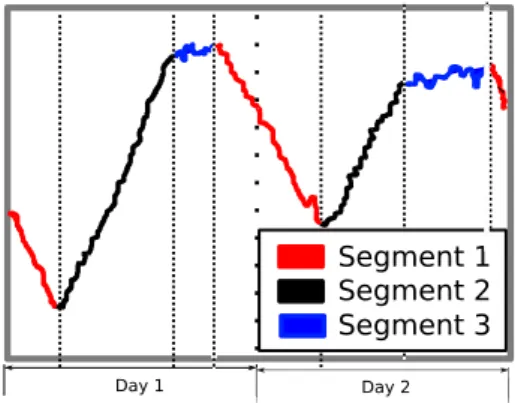
As a historical reference, one of the earliest works related to water time series forecasting, presents a multi-model application to water de-mand forecasting shown in the work of Shvartser in (SSF93). This work proposes a methodology based on pattern recognition and time series analysis; the daily consumption cycle is divided in three segments; ris-ing, oscillatris-ing, and falling. These segments are modelled separately and are seen as dynamical states. The sequence of the activation of each pat-tern associated with one state is modelled with a Markov process cap-turing the transition probabilities between states. Each segment of the time series with a specific pattern is associated with each state which is represented with a low order ARIMA model.

Figure 1 is an example of the decomposition of the time series in seg-ments. Segments number 1, 2, and 3 are classified as rising, oscillating, and falling respectively where the limits of the segments are defined by the dense dotted lines. Each segment may be occur during the day trans-action indicated by the pointy line. The pattern is observed throughout the information of two days.

Segment 1 Segment 2 Segment 3

Day 1 Day 2

(29)

S. Alvisi and M. Franchini (AFM07) developed a short-term, pattern-based model for water-demand forecasting. The model captures the pe-riodic patterns presented at annual, weekly and daily levels.

The model structure is based on the observed patterns at different ab-straction levels of the water demand time series. The forecasting struc-ture is hierarchically organised in two levels: The high level module that captures the low frequency patterns, like the seasonal and weekly pat-terns of the time series observed in Figure 1 from (AFM07). The low level model describes and predicts the daily consumption (Figure 3 presented in (AFM07)). In order to get the hourly forecasts over the next 24 hours period, a short term forecasting mechanism based on the combination of both models is implemented.

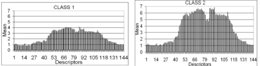
The work of J. Quevedo and V. Puig in (QSPB14) addresses a similar approach, where a Seasonal ARIMA (SARIMA) is used for predicting the daily water demand consumption combined with a descriptor class that distributes the amount of the predicted water consumption along one day. Mainly two validated descriptors are used. These descriptor classes are shown in Figure 2 and Figure 3, describing working and resting days patterns. These descriptors are validated using the LAMDA clustering method found in SALSA software package (KAS+_{03; Kem04). The}

pat-terns given by the descriptors are a priori assigned to each calendar day according to the human activity calendar.

Figure 2: Class 1 descriptor associated with weekend and holiday consumption patterns. ( c2014, IEEE).

Figure 3:Class 2 descriptor as-sociated with weekdays con-sumption pattern. ( c2014, IEEE).

(30)

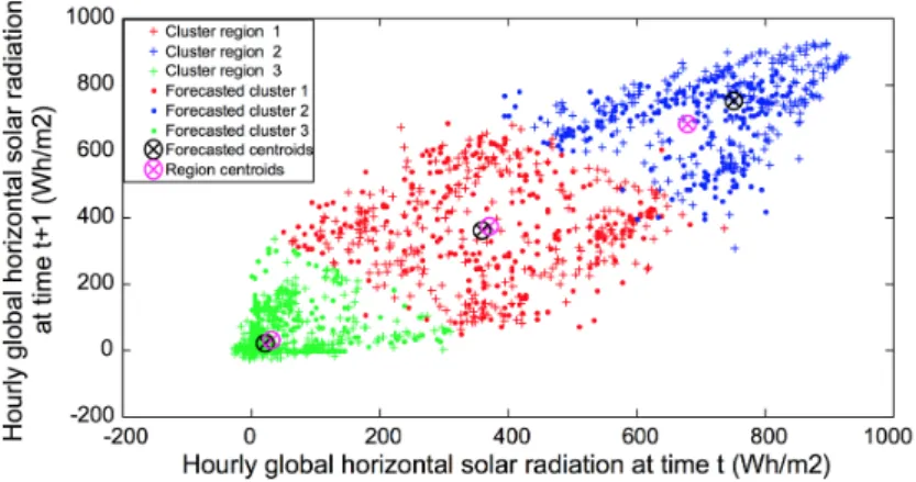
Benmouiza developed (BC13) a methodology based on the combina-tion of clustering methods and artificial neural networks to predict in the short term the solar horizontal radiation. The predictor model is a composition of several independent local models. Each model is trained with clustered data of one class containing similar dynamical patterns. The architecture has a Global Nonlinear Autoregressive Neural Network (NAR) used for predicting the local model to forecast. Once the local mo-del is selected, a local NAR momo-del associated with each cluster is used to forecast the hourly radiation. Although the application of the work aims to forecast the solar radiation, it might be possible to implement it for water demand forecast, since the dynamics of the water demand may obey also to global and local structure in its dynamics where the local dynamic patterns can be identified and clustered.

Figure 4 shows how the data in phase space is classified using a clus-tering algorithm finding three kind (or regions) of solar radiations. Each region represents low, medium and high solar radiation levels. A global NAR (Neural Auto Regressive) predicts the next region. Once the next region is estimated the local model forecaster related to the region is used to predict the radiation in an hourly basis. The dynamics of the hourly basis radiation is shown in Figure 5.

Figure 4:Phase space representation and clustered in regions of the hourly global horizontal solar radiation0_.

(31)

Figure 5: Measured hourly global horizontal solar radiation time series of July 19960.

M. Bakker et al. (BVVS13) propose a fully adaptive forecast scheme using a static calendar to compute in real time model weight coefficients (named day factors), and demand patterns used by the model. The mo-del assumes the existence of four kinds of different water demand pat-terns (reported in (ZAWL02)) of which those associated with holidays, weekdays, and holidays variations are known in advance but not the variants of season water demand patterns which should be detected on-line.

Another interesting approach based on the combination of multiple models, are the consensus and ensemble methods. The consensus mod-els are tools to create structured prediction maps which consider a lim-ited set of future forecasts based on expert information. This set of fore-cast are provided by the human knowledge (McN87). On the other hand, an ensemble forecast is a collection of two or more forecasts performed at the same time. These methods focus on generating scenarios that de-scribe probabilistically the predicted states of a dynamical system (LP08). Ensemble forecasting is considered a Monte Carlo analysis method where

0_{Energy Conversion and Management, Vol 75, K. Benmouiza,A. Cheknane, Reprinted from} Forecasting hourly global solar radiation using hybrid k-means and nonlinear autoregres-sive neural network models, Pages No 561-569, Copyright (2013), with permission from Elsevier

(32)

multiple numerical predictions are produced from generating different possible initial conditions given a past sequence and current set of obser-vations. Applications of these models are found in medicine (KOB13), health (FKCB84), economics, meteorology and water management. In economics, this approach is so relevant at the point that exists a spe-cialised firm named Consensus EconomicsTM_{group (Dat16) that collects} the state-of-the-art forecasters with their predictions for a big number of variables (more than 1000) from 85 industrialised countries in East-ern Europe, Asia Pacific and Latin America. The group has a signifi-cant community of researchers that confirm better accuracy of Consen-sus ForecastsTM_{than most of the individual forecasters (Bat00; BWWA01;} Jon14; NR11).

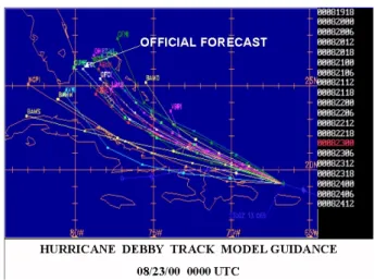
In meteorology, consensus forecasts are implemented to predict wea-ther and meteorological phenomena. As an example, Figure 6, a picture taken from the National Whether Service (Ser15), describes a category 4 Hurricane, Debby, that appeared in 1994. Each colored trajectory line, is a forecast simulation considering a randomised scenario. The set of fore-cast trajectories are used to produce a nominal prediction. This forefore-cast is the most likely trajectory that might be taken as official to predict the phenomenon dynamics.

Considering the survey of novel application in water management by Donkor et al. (DMSR14), the general concern of forecast methodologies is to fit the time series reducing the difference between the real value and the estimated forecast. Even though model fitting by minimising this gap is crucial to select a good forecasting model, the uncertainty prediction is also an important component for the forecast that should be considered in order to define the prediction bounds to give confidence to the predic-tion. With regard to water management, Tiwari et al. (TA15) propose a bootstrap method to learn a wavelet based machine learning considering also the minimisation of the prediction bounds. Other articles studying the uncertainty of stochastic models are found in (HK15), (CCK+_{08) and}

(AF14).

Based on the multi-modelling approach and the references collected regarding the design of multi-model forecasting, this thesis proposes the

(33)

Figure 6: Example of an application of ensemble forecasting applied to the prediction of hurricane trajectories.

next contributions to multi-model forecasting.

• The design of a module based framework that is able to exploit the empirical information using machine learning algorithms rather than the seasonal structure.

• Algorithms based on the exploitation of the historical information are useful as alternative to the existing modelling global methods.

• An implementation based on machine learning algorithms such as neural networks and clustering that identifies on-line different kinds of behavior patterns.

• Two implementations based on the qualitative and quantitative de-composition of the time series. Where the predicted quantitative in-formation is distributed along of an unitary pattern that describes a kind of activity (e.g, working or resting days).

– The first variation does not assume any a priory human in-formation about the water consumption modes and proposes

(34)

the use of a qualitative k-Nearest Neighbour (kNN) for mode prediction.

– The second implementation assumes the existence of an ac-tivity calendar used as predictor, but with the contribution of extending the method using a simple nonlinear filter to de-tect the qualitative pattern mismatches to readjust the pattern forecast along time.

This Chapter presented a brief historical introduction where George E.P. Box and G.M. Jenkins explored the decomposition of the data to anal-yse and understand time series dynamics to construct a stochastic model capable to predict time series with certain accuracy. After some research Casta ˜no et al. proved that a combination of unbiased forecasts gives reg-ularly a better unbiased forecast. Nowadays computational power gives the possibility to analyse and construct complex dynamics presented in time series. We addressed recent research in multi-modelling applied to time series from real sources as water demand, solar radiation, stock market fluctuations and meteorology. Next Chapter 3 addresses the com-mon forecasting methods and clustering algorithms oriented to system identification for our proposal.

(35)

Chapter 3

Time Series Forecasting and

System Identification

A time series is defined as a sequence of chronologically ordered obser-vations recorded at regular time intervals. The obserobser-vations are sequen-tial data that might represent qualitative or quantitative information de-pending on the source and application field. When the data are quantita-tive, the measurements that compose the time series express magnitudes or scalar information. An univariate time series notation used in the lit-erature is defined as follows in Equation 3.1:

Yf ull={Y1, Y2, . . . , Yt, . . . , Yn} (3.1) whereYf ull is the full time series,tis the index that indicates the time when the value was taken,nis the length of the time series. Usually time seriesYf ull, deals with scalar numbers that might be integers, reals, but sometimes they store qualitative information, where each element takes on a symbol from a defined set of objects. Yt ∈ A, whereAis a set of symbols included in the alphabet.

These measurements are taken via observations and then recorded somehow; for example manually or using computers that interact with electronic devices that record the information in data bases. The use of high speed computers and big storage allows to implement powerful

(36)

statistics and machine learning algorithms.

Time series forecasting is strongly related to system identification and modelling. System identification integrates statistical and mathematical tools to estimate and exploit the available information, and also studies the optimal design of experiments to generate informative data to fit dy-namical models. This is achieved by removing redundant or erroneous data keeping useful and descriptive information to model the object of study. This data treatment is useful for reducing the training or the pa-rameter optimisation time, and the model simplification.

The selection of information is important to control the detail level of the model according to the power and capacity of the implementation device: e.g., for small devices with limited memory and power process-ing a simple version of the model generated from the data should con-sider the most important characteristics of the object of study (as models implemented in microcontrollers for embedded control).

There are three levels of modelling abstraction in system identifica-tion. According to the scope of the and knowledge availability of the study object, the modelling levels can be classified as white, grey, and black-box modelling.

In white-box modelling, the dynamical processes are modelled us-ing differential equations to describe the motion of the system. Under this approach there is detailed and enough information to build an ac-curate model describing the nominal motion of the system of interest. This kind of modelling is useful for solving the implementation prob-lems of control, simulation and synthesis of the control law, especially in the space state approach. Typically, system identification is done by a human expert following laws and rules, for example the physical law of motion or chemical reaction laws. Although white-box is desirable in many cases due to the parsimony of the models, this approach has lim-itations when the systems are more complex or when it is not possible to have the precise parameter values for the system. In these cases the white-box methodology is not enough.

The next abstraction level of modelling is grey-box modelling. It ad-dresses those problems where the dynamical system is partially known

(37)

and the model is completed using empirical information. A typical case of grey-box modelling is when the general dynamic of the system is mod-elled but there are parameters that still need to be tuned. For example, the parabolic shot modelled with newton gravitational laws or hydro-logic model behaviours such as Nash-Sutcliffe and coefficient of deter-mination model efficiency (KBB05) (used to assess the predictive power of hydrological models). In this case, these parameters should be esti-mated using statistical methods with the available observations so far.

Black-box modelling is the highest level of modelling abstraction of the system identification approaches where there is little, no information, or unclear insight about the model behind that generates the sequence of observed data. This kind of modelling uses general purpose models tuned or trained using just the observed data. Examples of this kind of models are Auto Regressive (AR) models, Artificial Neural Networks (ANN) and Support Vector Machines (SVM) for discrete time modelling of continuous dynamical systems, or deterministic state machine for pi-ecewise models or Markov Chains Models for pipi-ecewise stochastic mod-els.

Once a model is obtained, it can be applied to simulation, control or forecasting of dynamical systems among others. The concept of black-box modelling abstraction is linked to the time series analysis that is the main focus of this thesis.

The main purpose of the time series analysis, is the design of dynam-ical models based on the empirdynam-ical observations of different phenomena. For the study of these observations, time series analysis provides the use-ful theory for the construction of methodologies and algorithms that are provided as tools for understanding the information for the correct mod-elling of the behaviour of the observed data.

During the analysis of time series two general approaches are taken into account depending on the linearity of the data, like the linear and nonlinear approaches. Linear methods are useful when the interpreta-tion of the observed data is regular presenting a dominant frequency and sequential information that can be measured with linear correlations. It is assumed that the systems are governed and explained with linear

(38)

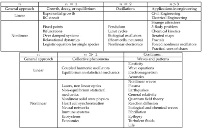
alge-bra theory. Using this approach the linear equations are limited to model systems that present a decaying, growing or damped periodically oscil-lating behaviour. The remaining irregularities are assumed to be random external inputs or disturbances to the system that can be described statis-tically by the normal distribution. Some examples of systems studied un-der this assumption are shown in Table 1 taken from the book Nonlinear Dynamical Systems in (Str94) of Strogatz and Steven H., where the dy-namics of the linear systems is determined and classified by the number of variables or differential equations. The basic systems belonging to this classification, present a simple growth, decay, or equilibrium dynamics when the dynamical systems contain one variable. When oscillations are present in the systems, they can be modelled with linear systems of two variables, for example, a simple mass-spring system. With more than three variables, applications are found in engineering e.g., coupled sys-tems modelled with several linear syssys-tems. For more complex syssys-tems like coupled oscillators require a greater number of equations or vari-ables to model them.

On the other hand, nonlinear methods address a more general family of dynamical models. This approach must be considered when the time series presents irregularities from the point of view of linear dynamical systems theory. The main drawback of linear theory is the impossibility to distinguish the random noise from the nonlinear structure of the data, therefore, it cannot model appropriately this kind of behaviour since the nonlinearity produces false residuals that might be confused with the noise where in reality it can be still modelled somehow. The systems in this category are natural processes. The simplest nonlinear models that contain just one variable are used to study fixed points, bifurcations, over damped systems or the equilibrium in ecosystems. For two variables nat-ural oscillations, like limit cycles, biological oscillations, and nonlinear electronics are studied. For three or more variables, systems that might present strange attractors, chemical kinetics, iterated maps or fractals are studied. For many variables the nonlinear optics, non equilibrium sta-tistical mechanics, heart cell synchronisation, biological neural networks response, complete ecosystems and economics behavior are studied. For

(39)

the continuum domain, nonlinear waves, plasma, earthquakes, general relativity, quantum field theory, reaction diffusion, biological and chem-ical waves among others systems are studied.

Table 1:Classification of the dynamical systems according to their number of variables

n n= 1 n= 2 n>3

General approach Growth, decay, or equilibrium Oscillations Applications in engineering Linear Exponential growth_{RC circuit} Civil Engineering_{Electrical Engineering}

Nonlinear

Fixed points Bifurcations Over damped systems Relaxational dynamics Logistic equation for single species

Pendulum Limit cycles Biological oscillators (Heart cells, neurons) Nonlinear electronics Strange attractors 3-Body problem Chemical kinetics Iterated maps Fractals

Forced nonlinear oscillators Practical uses of chaos

n n1 Continuum

General approach Collective phenomena Waves and patterns Linear Coupled harmonic oscillators

Equilibrium in statistical mechanics Elasticity Wave equations Electromagnetism Acoustics

Nonlinear

Lasers, non linear optics Non-equilibrium statistical mechanics

Nonlinear solid state physics Heart cell synchronisation Neural networks Immune systems Ecosystems Economics Nonlinear waves Plasma Earthquakes General relativity Quantum field theory Reaction diffusion Biological and chemical waves Fibrillation

Epilepsy Turbulent fluids Life

All the mentioned systems are able to generate a time series since it is possible to measure the states of certain variables along time. For this reason the study of time series is also strongly related to the study of nonlinear dynamical systems when they come from natural or artificial systems.

The present thesis is related to dynamical systems difficult to mo-del analytically belonging to nonlinear systems family. The momo-dels are obtained using different technics with the final objective of producing accurate forecasts.

A special case of nonlinear systems are the piecewise linear or non-linear dynamical systems, where the system is modelled by a set of local models that are activated by certain rules. Each local model is associated with one operation mode. The activation of these local models depends on the model of the finite state machine in the deterministic case (Bla08), or by a stochastic state machine that activates the different local

(40)

mod-els by probabilistic rules such as those performed by Markov Modmod-els Chains. Figure 7 shows an example of a finite state machine model that captures the dynamics of behavior changes. The submodels or states are activated when an event occurs. In contrast, the Markov Model (GS10) in Figure 8 models the change of states by producing probabilities events to jump from one state to another.

Figure 7:In a finite state machine transition states are triggered by events.

Figure 8:In Markov Model transition states are triggered with certain prob-ability.

The next subsection addresses the basics of linear time series analy-sis introducing its basic components, a general methodology to extract them, and some notes about stationarity and sampling that remarks the importance of selecting the correct data to the study and modelling of time series.

(41)

3.1 Linear Time Series Analysis

Linear time series analysis studies time series that can be modelled by analysing and identifying the secular trend, seasonality, and noise com-ponents. A popular and simple way to analyse the dynamics is by us-ing Auto-Regressive time series models. These models are a standard in modern stationary time series data analysis (MJK08). The advantage of these models is that they are seen as a combination of components of larger models that leads to generalised forms.

Although it has limitations for nonlinear time series, the concepts and structure of linear models provide a background for the analysis of non-linear models. Univariate time series also can be classified according to their domain in frequency based methods and Time domain based meth-ods.

Regarding time domain based methods the time series are studied from the stochastic process point of view. A stochastic process is a se-quence of random variablesYttaking any value from[−∞,∞]wheret is interpreted as the time in the discrete domain. Given a sequence of values each of theYt variables have their own function that captures their distribution within of their corresponding moment. Each pair of these variables will have their corresponding joint distribution and the marginal distribution functions.

These time series can be decomposed to be analysed by its three com-ponents: the trend (long term direction), the seasonal (systematic, cal-endar related movements) and the irregular (unsystematic, short term fluctuations) components.

In order to proceed with the description of some of the most popular methods used in the literature as Box-Jenkins and Holt-Winters, basic definitions are defined next about the structure of the linear time series.

i Secular trend is the persistent component of the observed phenom-ena; it describes the long-term trend. The appearance of this com-ponent is exemplified in Figure 9 where the red line shows the long-term trend. Although for simplification a linear fitting is used, it is also common to observe a long-term nonlinear trend (e.g.,

(42)

exponen-tial or geometric growth). Some examples of secular trend cases can be global warming, inflation in economy, increase of energy and con-sumption and decrement of the availability of the water resources along the time.

50 100 150 200 t 2 4 6 8 10 12 14 Y

Figure 9:Secular trend

ii Seasonality variation describes the short-term periodic movement. An example of how this component looks is presented in Figure 10. Some examples where this component is present are daily variation of the temperature, daily sea level and water demand in a short term.

iii White noise is modelled by a normal distribution function that cap-tures the random variation of variables. This component also has the property of having zero mean, constant and independent variance for different values along time. An example of what the noise com-ponent looks is shown in the Figure 11. White noise can be presented as external disturbances, error measurements due to technical limita-tions and interference.

iv Transient variation captures the accidental dynamic presented reg-ularly as isolated perturbations or aperiodic fluctuations that affect the regular behaviour over the time. An example of the appearance

(43)

50 100 150 200 t -2 -1 1 2 Y

Figure 10:Seasonal variation

50 100 150 200 t -1.0 -0.5 0.5 1.0 1.5 Y Figure 11:Noise

of this component is shown in Figure 12, where aperiodic oscilla-tions are present. It is possible to confuse this component with noise. When it appears, a nonlinear model might be used for describing the dynamics of this component.

In the time series classical analysis literature, decomposition is used to describe separately the trend and seasonal factors. Linear modelling can be classified according to the way of combining these components

(44)

50 100 150 200 t -0.2 -0.1 0.1 0.2 Y

Figure 12:Transient variation

in additive, multiplicative and pseudo additive compositions (HA13). Another kind of decompositions focuses on describing long-run cycles, like the weekends and holiday effects (QSPB14). The classification of time series according to their decomposition is:

i Additive models consider the sum of the trend, seasonal, and ran-dom variation. It is used when the seasonal variation is relatively constant over time. It is expressed by Equation 3.2

Yt= T + S + R (3.2)

where the times series is generated by addingT,S, andR, the trend, seasonal, and random components respectively. An example of the general structure of this model is shown in Figure 13.

In this figure the red line is the trend approximation of the time se-ries, and the black line is the real data with seasonal components and noise.

ii Multiplicative models are composed by the multiplication of the dif-ferent components like trend, seasonal and random components. This kind of model is used when an increasing seasonal variation is ob-served along the time. It is expressed by Equation 3.3.

(45)

50 100 150 200 t 5

10 Y

Figure 13:Additive composition example

Yt= T×S×R (3.3)

where the componentsR,SandTare the same described previously, with the difference that the time seriesYtis the result of the product of such components. An example of the structure using this kind of decomposition is shown in the Figure 14.

50 100 150 200 t -6 -4 -2 2 4 6 Y

Figure 14:Multiplicative composition example

(46)

variance of the time seriesYt.

iii The pseudo-additive decomposition (Mixed) presents a more com-plex dynamic, adding and multiplying the different components. It combines features of both the additive and the multiplicative models. The general structure of this kind of model is expressed by Equation 3.4:

Yt= TCt×(S + I)−1 (3.4)

where the addition of the seasonal effects, and irregular fluctuations

(S + I)−1produces a trend in the mean, and the trend cycle compo-nentTCtproduces a multiplicative effect that increases the variance along time. Figure 15 shows an example of how a time series of this type looks like. The low and high red dotted line bound the time se-ries according to an increasing variance. The continuous red line is the mean increasing along the time.

50 100 150 200 t 5 10 15 20 Y

Figure 15:Pseudo-additive time series example

3.1.1 Decomposition Methodology in Classical Analysis

In time series classical analysis, it is important the study of different com-ponents present in time series separately. Although time series analysis

(47)

may be considered a sort of art, it requires statistical knowledge, the-ory and good practices for generating a valid and correct model. Box and Jenkins proposed a methodology to understand systematically how a time series behaves following adivide and conquerstrategy (BJR94). De-composing the data in simpler time series is crucial to identify and esti-mate the different components involved in the time series. An important assumption to consider is the generation of the data by a linear dynami-cal system. Considering the different components the general steps that should be taken into account, according to Box and Jenkins are:

i Observation: This step is the most important because with visual analysis is possible to have the intuition and information about gen-eral aspects of the data useful for selecting the proper gengen-eral model to use.

ii Trend estimation: To detect the estimation in the long term in time series can be used mainly two different kind of methods belonging to different approaches:

• Filtering: It is a function capable of neglecting the short term dynamics and keep the general dynamics. An example of this kind of algorithms is the smoothing effect of a moving average.

• Estimating a regression equation: A (linear or nonlinear) func-tion might be used to describe the trend using least squares op-timisation (Sch13). (Like the solid red line in Figures 9, 13 and 15).

iii De-trending: When the trend is already known, for the additive com-position the trend is removed subtracting it from the original time series. For the multiplicative composition the trend is removed di-viding the time series by the trend.

iv Detection of seasonal factors: If the seasonality is known, the sim-plest method for estimating these effects is to average the de-trended values for a specific season using the Seasonal Sub-series Plot, other-wise a correlation plot helps finding the seasonality (Cle93) .

(48)

v Determine the random (irregular) component: The random compo-nent is analysed last. After obtaining the forecasting model, the vari-ance of the noise by means of gaussian random distribution is anal-ysed.

series. Matlab does this (and estimates the trend with a straight line in the iteration.

3.1.2 Stationarity and Sampling

In order to study a phenomena it is important to reproduce it many times under the same conditions and be sure that the measurements taken ef-fectively correspond to the same scientific study, object, or process. The concept of reproducibility in time series is strongly related to invariabil-ity and availabilinvariabil-ity meanings.

1. Invariability of parameters during the analysis of the system: These parameters must not depend on time and they change once they are noticed or desired to produce intentionally an output.

2. Availability of the data addresses the problem of the incorrect mod-elling due the lack of information which impedes to detect and con-sider the non-stationarity of the process. Non-stationarity is dif-ficult to detect and model since it is also difdif-ficult to know if the acquired information is enough and reliable providing a good de-scription of the general dynamic of the data.

When the phenomena is studied a finite number of times and behaves differently we can also say that it represents a non-stationarity process, and presents an intermittency effect. The intermittence is observed only if we can replicate the process enough times. Conversely, the analyst will not have enough data to produce a reliable model. Therefore, the length of the series must provide enough information to describe and take into account intermittency.

(49)

3.1.3 Testing for Stationarity

The stationarity test is performed over stochastic processes. The simplest non-periodic stochastic process, is composed by a set random variables

{Yt}t∈O, whereYt ∈ R,t is the time index included in the setO, with

infinite values in the interval(0,∞]in a continuous-time. For discrete-time process the random variable takes a finite number ofNvaluesO=

(0,N], restricting the length of the discrete time series. A stationarity

process is present when the probabilities related to the random variables are constant over time. This is expressed in Equation 3.5.

P r(Yt+τ) =P r(Yt) (3.5)

where P r is the probability of observing certain value, and {Yt, Yt+τ,

. . . , Yt+psτ}are the observations belonging to the same probability

dis-tributionP r(Yt).

Stationarity is confirmed when there is no violation of the basic prop-erties of the stochastic system like variance, mean, transition probabili-ties, and correlations. Considering the difficulty for detecting stationar-ity for periodic time series, it is recommended to get considerably longer data length than the period length for modelling to capture as much cyclic samples as possible. As soon as we get large data, we will have more chances to determine and distinguish the global trend, patterns and intermittence effects. This means that the sample data size must be greater than the period,τ.

In other words we need a large data set of sizen, such thatnpsτ, whereτ is the size of the period andps is the number of periods that guaranteepcharacteristic samples, e.g., Figure 16 gives the impression of non-stationarity only if the data we have is limited, therefore it is not possible to determine periodicity. On the other hand, if we have more data, like in Figure 17 a pattern is revealed. Hence local stationarity is detected. Figure 17 shows complete cycles with a relative stationarity (since we do not know what will happen in the future).

Assuming we have sufficient information, we can take two appro-aches for testing stationarity: the parametric and nonparametric

(50)

app-2 4 6 8 10 12 Time in Hours 0.12 0.14 0.16 0.18 0.20 0.22 Water Consumption

Figure 16:Incomplete pattern

20 40 60 80 Time in Hours 0.15 0.20 0.25 Water Consumption

Figure 17: Four complete pat-terns

roach. The parametric is usually used by researchers considering sta-tistical assumption about the distribution of the data in the time field domain, such as economists and statesmen. Such assumptions can be tested according to the 1st or 2nd order stationarity criteria.

• 1st order stationarity is related to strict stationarity criteria. It as-sumes a time-independent joint statistical distributions and vari-ations of the time series, therefore, the mean and variance at any moment must be the same. Strict stationarity satisfies Equation

[P r(Yt1+τ0), . . . , P r(Ytns+τ0)] = [P r(Yt1), . . . , P r(Ytns)]

where the probability of the shifted vectors satisfies the equality independently of the chosen value ns, t1, . . . , tns ∈ O, or lag τ

0

(LRS13).

In real time series this definition is very tight and time series pre-senting some irregularities almost never satisfy this condition.

• 2nd order stationarity is about relaxed stationarity condition. It is more flexible and considers a stationary process only if the mean (first moment) is constant and covariance (second moment) is finite and depends just on the time differenceτ0=t−t0along time series.

The nonparametric approach does not require any assumption of the data, therefore it is more general. One of the most popular stationarity

(51)

test is the Runs Test. The test defines a run as “succession of one or more identical symbols or patterns”, which are followed and preceded by a different symbol or no symbol at all (Gib83). The idea behind is similarly to a series (or runs) generated by identical flips of a coin, where the sym-bolOandIrepresents heads and tails, respectively. An example of such run is the sequenceC={OIIIIIIOOIOO}. If the coin is balanced, the sequence will present stationarity approximating the same number ofO

andIas long as more observations are available, otherwise a trend might be detected.

The stationarity of data can be determined by using the algorithm of the runs test proposed by Bendat and Piersol in (BP86) as follows:

1. Divide into intervalsTof lengthτ.

Z_T0 ={Yt}T τt=τ(T−1)+1 (3.6)

2. Compute a mean value for each interval.

Z0_T = 1 τ τ X t=1 (Z_T0) (3.7)

3. Collect the occurrences of values above (I) and below (O) the me-dian valueZ˜0_{of the series using Equation 3.8.}

CT =

(

I ifZ0_T >Z˜0₎

O otherwise (3.8)

4. Count the number of runs withIandOfollowing Equation 3.9

CO=|{i,∀i∈ {1,2, . . . , T−1, T},|Ci=O}| (3.9)

CI =|{i,∀i∈ {1,2, . . . , T −1, T},|Ci=I}|

5. Compute the probability of having a runP r(CO₎_and_{P r}_(CI₎_and ifP r(CO)≈P r(CI), the the stationarity test is passed.

(52)

3.1.4 Linear Autocorrelations

We have seen so far how the general characteristics of the time series are analysed discarding dynamic details at local level. In order to analyse what is going on with the observed dynamic fluctuations at local level of the time series, a relation analysis between variables is performed.

The relation analysis is an important part of the study of linear time series, it focuses on the existence of a linear temporal relation between the the variable of interest and another one is named autocorrelation.

There are two kinds of autocorrelation metrics used as tools for mea-suring the existence and intensity of such correlation among the data, the simple and partial autocorrelation.

• The Simple Autocorrelation Function (ACF), measures the lineal relation between the observationYtfrom a time series and the de-layed valueYt−τ.

• The Partial Autocorrelation (PACF), is the estimation of the simple correlation but removing the effect produced by the autocorrela-tions for delays shorter thanτ.

The degree of relation for the simple and partial autocorrelation is measured using the autocorrelation coefficientρτ. The coefficient takes values in the interval[−1,1]. This coefficient provides information about the existence and the type of correlation. A coefficient with value of+1

means a strong positive relation between two observations separated by

k units of time. The positive sign means that both variables respond similarly. A value of−1expresses a strong inverse relation. When a value of0is obtained, the two variables do not exhibit any relation. Equation 3.10 computes the autocorrelation function.

ρτ =corrττ(Yt, Yt+τ) =

γτ

γ0

(3.10) wherecorris the autocorrelation function at lagτ,ρτis the coefficient of the simple autocorrelation for a delay ofτ, andγ is the covariance function defined in Equation 3.11

(53)

γτ =cov(Yt, Yt−τ) =E[(Yt−Y)(Yt−τ−Y)] (3.11) wherecov is the covariance function,Y is the mean of the time series,

Yt−τ is the observation at lagτ,Eis the expectation andγ0is equal to 1

by definition following Equation 3.12

γ0=var(Yt) =ρ0= 1 (3.12)

wherevaris the variance. This property is found in (Fra85).

The Partial Autocorrelation Function (PACF) ofτ order is similar to the ACF that measures the correlation between two variables Yt and

Yt−τ, but with the difference of discarding the influence of the depen-dency of the intermediate lags between both of them. The partial auto-correlation gives information about the AR order. The recursive formula proposed by Levinson and Durbin (Fra85) is described in Equation 3.13

ˆ π11 = ρ1 (3.13) ˆ πτ,τ = ρτ−P τ−1 j=1πˆτ−1,j∗ρτ−j 1−Pk−1 j=1πˆτ−1,j, ρτ−j

where ˆπτ,j = ˆπτ−1,j −ˆπτ,τπˆτ−1,τ−j is the covariance at different lags

j= 1,2, . . . , τ−1.

Equation ACF 3.10 and PACF 3.13 are used to produce plots named autocorrelograms. Each autocorrelogram is composed plotting the coef-ficientsρτ andπˆτ,τ respectively varyingτ at different lags. Each auto-correlogram provides information about the Moving-Average (MA) and Auto-Regressive (AR) polynomial order and structure (BJR94). The de-scription of the Box-Jenkins ARIMA methodology is addressed in Chap-ter 3.2.

The Ljung-Box test is an auxiliary test born in 1970 (BP70) and imple-mented to quantify the model fitting (LB78) measuring the independency of the values of time series. This test gives information about the possible existence of linear relations in the data or if the data sequence is merely random noise. The Ljung-Box test is given by Equation 3.14