Mining Interesting Subnetworks from Graphs with Node Attributes

(1)

MINING INTERESTING SUBNETWORKS FROM GRAPHS WITH NODE ATTRIBUTES

A Dissertation

Submitted to the Graduate Faculty of the

North Dakota State University of Agriculture and Applied Science

By

Aditya Praneeth Goparaju

In Partial Fulfillment of the Requirements for the Degree of

DOCTOR OF PHILOSOPHY

Major Department: Computer Science

April 2018

(2)

NORTH DAKOTA STATE UNIVERSITY

Graduate School

Title

MINING INTERESTING SUBNETWORKS FROM GRAPHS WITH NODE ATTRIBUTES

By

Aditya Praneeth Goparaju

The supervisory committee certifies that this dissertation complies with North Dakota State Uni-versity’s regulations and meets the accepted standards for the degree of

DOCTOR OF PHILOSOPHY SUPERVISORY COMMITTEE: Dr. Saeed Salem Chair Dr. Kendall Nygard Dr. Simone Ludwig Dr. Mukhlesur Rahman Approved: April 20 2018 Date Dr. Saeed Salem Department Chair

(3)

ABSTRACT

A lot of complex data in many scientific domains such as social networks, computational biology and internet of things (IoT) is represented using graphs. With the global expansion of internet, social networks had an explosive growth with billions of users in FaceBook. Similarly research in Bio-informatics generated massive amounts of genomic data (protein protein interaction networks) from several high throughput techniques. Due to the large amount of data involved, researchers have turned to data mining techniques to discover meaningful and relevant information from large graphs.

One of the most intriguing questions in graphs representing complex data is to find commu-nities or clusters. The members in a clusters have high density of edges to other members within the cluster while very low edges to members outside of the cluster. Real world graphs often have additional attribute data characterizing either the nodes or edges of a graph, such as age or interests of a person in a social network. Recent research has combined the problem of community detection with subspace similarity over attribute data. For example, in the context of social networks, we might be interested in finding groups of friends who are of similar age and share common interests. The use of attribute data in finding clusters is shown to be eﬀective in many application areas such as targeted advertising in social network or detecting protein complexes in protein protein interaction networks which might be indicative of diseases such as cancer.

In this dissertation, we propose multiple algorithms for mining communities with similarity in attributes from node-attributed graphs. Experiments on real world datasets show that the proposed approach is eﬀective in mining meaningful clusters.

(4)

ACKNOWLEDGEMENTS

I would like to express my thanks to my advisor Dr. Saeed Salem for supporting me during all these years. He has been a tremendous mentor, his advice and help during my research has been invaluable. I would like to thank him for encouraging and helping me in my research, without which this research wouldn’t have been possible. I would like to express my gratitude to all my committee members, Dr. Hyunsook Do, Dr. William Perrizo and Dr. Gokhan Egilmez, Dr. Kendall Nygard, Dr. Simone Ludwig and Dr. Mukhlesur Rahman for taking the time to evaluate my project and helping me to graduate from the University.

I also want to express my thanks for North Dakota State University and the Department of Computer Science for oﬀering me the opportunity to study at such a great school. The people and the environment have made it a great place to study and learn.

I thank my fellow students, Kutub Syed and Tyler Brazier, Ming Chao and Bassam Qormosh for working with and beside me during my research. Lastly I also want to thank my wife for supporting and encouraging me through out this journey.

(5)

6.2.1. Cohesive communities with noisy node attributes . . . 67 6.2.2. Cohesive communities with edge attributes . . . 67 6.2.3. Cohesive communities with ranked edge interaction data . . . 68 6.2.4. Sampling cohesive communities with multi relational edge attribute data . . 70 6.2.5. Parallel approach to sampling . . . 72 REFERENCES . . . 75

(9)

LIST OF TABLES

Table Page

3.1. Topological properties of cohesive dense clusters for Yeast dataset. . . 26

3.2. Topological properties of cohesive dense clusters for Biogrid dataset. . . 29

3.3. Similarities of medoids in Representative Set. . . 33

4.1. Topological properties of cohesive clusters for the YeastHC dataset. . . 43

5.1. Summary statistics of the visit counts of the samples in uniform sampling which includes minimum, maximum, mean and standard deviation of the visit counts. . . 59

5.2. Results of sampling algorithm on Yeast dataset. . . 60

5.3. Results of sampling algorithm on Human dataset. . . 62

5.4. Traversal of enumeration and sampling algorithm. . . 62

5.5. Biological enrichment analysis on modules generated by sampling algorithm in human dataset. . . 64

(10)

LIST OF FIGURES

Figure Page

2.1. Visualizing communities in a sample web site graph . . . 6 2.2. Enumeration tree example. (a) A sample graph. (b) Enumeration tree for the sample

graph; node order 1<2<3<4 is followed while generating child nodes. . . 9 2.3. Graph with node attributes and two cohesive communities. . . 10 2.4. Graph with edge attributes and two cohesive communities. . . 11 3.1. Example node attribute graph. The graph shows two communities, vertex 4 belongs to

both communities. . . 13 3.2. Example graph (a) and its enumeration tree (b). θ= 0.7. Crosses show which branches

are pruned. The discovered maximal clusters are in green. . . 16 3.3. The input graph and its corresponding enumeration tree. There are four threads which

build the enumeration tree independently. There are 4 threads and each thread builds subtree for 2 first level children. . . 19 3.4. Finding representative clusters. (a) The maximal cohesive clusters. (b) The cluster

similarity graph for α = 0.5, edges show dissimilarity between clusters; (c) Applying k-medoids algorithm results in finding clusters and medoids (highlighted in blue), edges show distances between clusters. . . 21 3.5. Representative clusters. (a) Set of maximal cohesive dense clusters, (b) Projecting

maximal cohesive dense clusters to points in space. (c) Finding partitions around the random medoids. (d) Detecting steady state medoids m1 =P3 and m2 =P2 and its partitions c1 and c2 respectively. The representative maximal cohesive dense clusters are the set of steady state medoids m1, m2 . . . 23 3.6. Functional interpretation of patterns: GOTERMs and KEGG pathways enrichment for

the YeastHC dataset fort= 0.3, smin= 30. . . 27

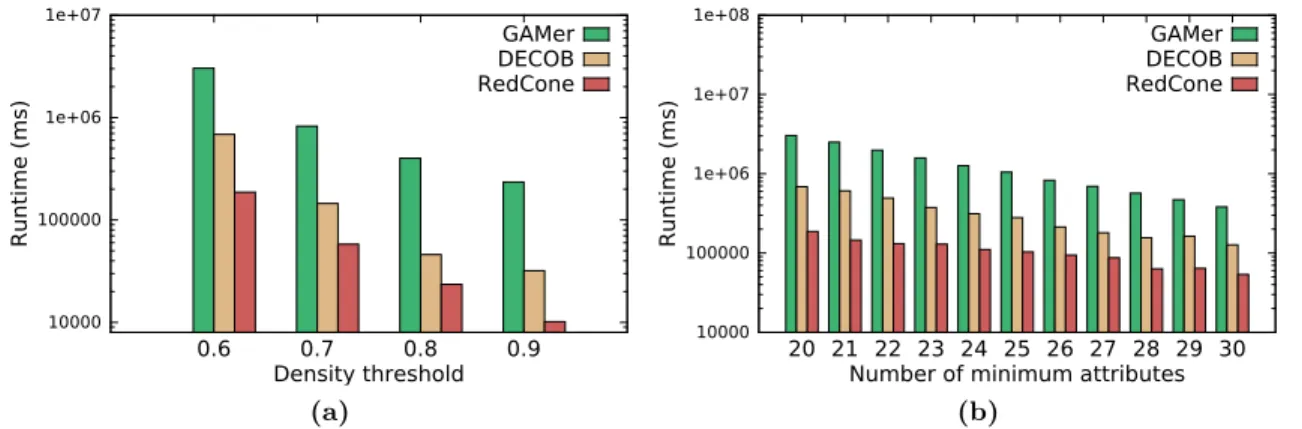
3.7. Representation of a dense and cohesive patterns from the YeastHC dataset, showing their network structure and attribute similarity of nodes in each pattern (a) number of vertices = 8 (b) number of vertices = 9; Parameters: θ = 0.7, t = 0.5 and smin = 20 (Only 40 attributes are shown) . . . 28 3.8. Runtime comparison of GAMer, DECOB and RedCone on the YeastHC dataset (a)

parameters : t= 0.4 andsmin= 20 (b) parameters : θ= 0.6 andt= 0.4 . . . 28

3.9. Runtime comparison of DECOB and RedCone on the BioGRID dataset (a) parameters : t= 0.4 andsmin = 60 (b) parameters : θ= 0.7 and t= 0.4 . . . 29

(11)

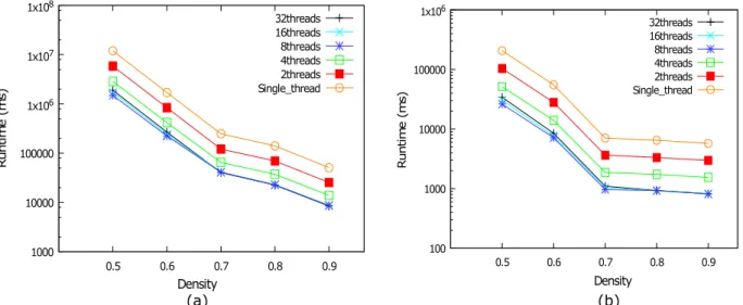
3.10. Runtime comparison of multiple threads on the Yeast dataset with varying density, parameters : (a) t= 0.4 andsmin = 60 (b)t= 0.3 andsmin= 65 . . . 31

3.11. Runtime comparison of multiple threads on the Yeast dataset with varying dimension, parameters : (a) t= 0.4 andθ= 0.9 (b) t= 0.4 andθ= 0.7 . . . 31 3.12. Runtime comparison of multiple threads on the Human dataset with varying density,

parameters : smin= 4 . . . 32 3.13. Runtime comparison of multiple threads on the Human dataset with varying dimension,

parameters : θ= 0.6 . . . 32 3.14. Average intra partition similarityAvgP artitionSimand average inter medoid similarity

AvgM edoidSimwith varying alpha values. . . 33 3.15. Average intra partition similarityAvgP artitionSimand average inter medoid similarity

AvgM edoidSimwith varying K values. . . 34 4.1. Example of cohesive network. Graph containing two communities, (a) An example of

dense cohesive subgraph and (b) an example of a cohesive subgraph . . . 35 4.2. MinCone approach.(a) Sample enumeration tree where A, B, U, U∗ are all cohesive

clusters, clusterU is the parent of the clusterU∗ (b) cohesive cluster represented byU

(c) child cohesive cluster represented byU∗ (d) MST of U∗. . . 39 4.3. The input graph and a portion of the corresponding enumeration tree built by MT Mincone

. There are four threads which build parts of the enumeration tree independently. Each thread builds two subtrees from the first level children. Crosses show which branches are pruned. The discovered maximal cluster is highlighted by a green box. . . 41 4.4. Representation of a cohesive pattern from the YeastHC dataset (a) Network structure

of the pattern (b) Attributes of the nodes in the pattern; Parameters: t = 0.4 and

smin = 40 (Only 80 attributes are shown). Notice the pattern is not particularly dense . 44 4.5. Runtime comparison of brute force approach and MineCone on the YeastHC dataset (a)

parameters : t= 0.4 (b) parameters : smin= 40 . . . 44 4.6. Speedup in runtime for multiple threads (a) on the Yeast dataset with varying dimension

while tolerance is fixed att= 0.35 (b) on the Yeast dataset with varying tolerance while dimension is fixed atsmin= 30 (c) on Human dataset with varying dimension . . . 45

5.1. (a) Module enumeration process enumerates all modules from the input graph. Modules are shows as circles and representative modules are shown by filled circles. Summariza-tion process then tries to reduce this exponential output set to a representative set. (b) Sampling technique outputs a reduced set directly from the input graph database without enumeration. . . 48 5.2. A input graphGand the corresponding POG represented byM, assuming every module

(12)

5.3. Uniform sampling where |N| = 107, sampling algorithm ran for 10700 iterations (a) Visit counts of each sample (b) Histogram of visit counts . . . 59 5.4. Targeted sampling where |N|= 3819, sampling algorithm ran for 75000 iterations (a)

Visit counts of each sample (b) Scatter plot graph between score of the module and the visit count of each module. The blue line indicates the positive correlation between score of the module and visit count. . . 60 6.1. Graph with edge attributes and two communities. . . 68 6.2. Graph with ranked edge attributes. The dashed ellipse shows a community formed by

including the topics from a broadcast message. . . 69 6.3. A graph containing multi relational edges, (a) An example of co-authorship network

where two authors co-authored a paper and (b) an example of citation network where authors cited each other. In this example the community formed by{1,2,5,6} is dense in both co-authorship and citation network with a minimum density of 0.6, assuming they are cohesive in their edge attributes . . . 70 6.4. DBLP graph. (a) An example DBLP graph with multiple relational edges, solid edges

are co-authorship and dashed edges are citation edges. (b) Partial order graph for input graph in (a) with co-authorship topology. (c) Partial order graph for input graph in (a) with citation topology. Notice that subgraph{A, C}does not exist in POG for citation topology. . . 72 6.5. Multi threaded approach to sampling inP OGwith two threads (Th1 and Th2)

perform-ing parallel random walk. Each thread is restricted to its respective area highlighted by color. . . 73

(13)

1. INTRODUCTION

Biological, social and technological networks have been modeled as graphs, and graph anal-ysis has become crucial to understand these complex systems. In each of these areas, a vertex represents a gene, person or a node and their interaction or relationship is represented by an edge. Often these vertices or edges have properties associated with them which can be modeled as at-tributes. These properties for example, can represent the personal profile attributes such as age or interests of a person in a social network or gene expression data which encodes information that can determine the dysregulation of a gene in a disease [21].

One of the most intriguing questions in graphs representing complex data is to find commu-nities or clusters [26]. Commucommu-nities are groups of vertices of a graph that have a high concentration of edges within the group and very low concentration of edges between these groups. With the availability of attribute data it is highly desirable to find communities which also exhibit similarity over its attribute data. A community can be viewed as an independent region of a graph, where all the vertices or edges exhibit similar properties or behavior. Communities that have a dense network structure and maintain attribute similarity are called cohesive communities.

Cohesive community detection has received some attention recently [77, 36, 30], however, this concept is still fairly new and requires further study. Most of the recent research have some sort of limitations. Some approaches use a stricter representation for communities which might miss some interesting communities. While some other approaches are not very flexible in handling attributes. This research attempts to address the question of detecting cohesive communities while maintaining a subspace similarity over real (floats) attributes.

Detecting communities is very essential as communities have many practical applications [26]. A community in a protein protein interaction network can represent biological complexes which can be used to diagnose diseases [70]. A community of friends in a social network with similar interests can be targeted for advertisements or recommendations [79]. With such an ever increasing list of applications it is very critical to find novel ways to detect cohesive communities with attribute data over nodes or edges.

(14)

In this paper we discuss new approaches to find cohesive communities in rich graphs. We first define what cohesive communities mean and then show techniques to mine cohesive communities from a graph. We also compare our technique against the state of art algorithms and present our results.

1.1. Motivation examples

In this section we shall discuss some motivational examples for the application of commu-nities in various fields of science and establish their importance. Furthermore we also see how integrating the definition of communities with similarity of attributes is proving to be further beneficial.

1.1.1. Biology

In bioinformatics, the interactions between proteins is generally represented as an interac-tion graph known as protein protein interacinterac-tion (PPI) network, where nodes represent proteins and edges represent pairwise interactions between them. Application of network clustering methods had significant impact which have led to extraction of functional modules such as protein complexes [60] or regulatory pathways [64]. These complexes are a cornerstone of many biological processes and together they form various types of molecular machinery that perform a vast array of biological functions, such as finding targets for antimicrobial drugs [60]. These complexes or clusters are proving very useful in identifying potential biomarkers in a variety of diseases such as Tuberculo-sis, Pediatric Pneumonia and Pulmonary Sarcoidosis [6, 78, 53]. Recent research in bioinformatics shows that integrating gene expression profiles with the PPI network structure improves diagnosis and prognosis of cancer [15, 16]

1.1.2. Social networks

The development and analysis of social networks and the application of graph theory in sociology has been studied since the early 1900’s [27]. Social network analysis produces an alternate view, where the individuals are less important than their relationships with other actors within the network. This approach has turned out to be useful for explaining many real-world phenomena [75]. As social media is gaining popularity [2], billions of online profiles (attributes) exist on popular websites like Facebook, Twitter, etc. Combining community detection with attribute data has given rise to multitude of applications in the recent times. Behavior and sentiment analysis during elections [68, 69], location-based interaction analysis [80, 14] and marketing and recommender

(15)

systems development like used in Facebook [13] are some of the applications that stem from social network analysis.

1.1.3. Enron email data set

Enron email data set is a large corpus of emails generated by employees of the Enron Corporation which was later used for investigation after the company’s collapse. The original dataset contains 619,446 email messages [46]. A subset of the original data has been normalized and annotated with category labels by UC Berkeley [25]. This subset of data contains 1700 email messages and each email is categorized with three labels from a set of 53 labels. An email network was constructed from this email data set where nodes represent employees and edges represent an email communication between the employees. The category labels on the email were associated to the edge attributes. Finding dense communities who frequently exchange emails with “financial bankruptcy” or “fraud” topics can be extremely useful to investigators who can localize their search to people who participate in certain key topics [62].

1.1.4. Developer networks in open source software

In software engineering developers collaborate to work together and in doing so they form inherent developer networks [39]. Code review is a process in which the author of a specific code asks others relevant expert developers to review the code before submitting to the code repository. The code review process in open source software is diﬃcult because of the distributed and voluntary participation of developers. Finding a cluster of relevant expert developers who can review code related to a specific area is one of the big challenges in this space. In a developer network, each node represents a developer and an edge is drawn between two developers when they co-comment on a code review. The class or modules that a developer has reviewed and commented are modeled as the node attributes for that developer, indicating their expertise. The problem of finding a relevant set of expert developers can be reduced to the problem of finding communities in the developer network who have similar attributes.

Community detection is very essential as is made evident by the preceding examples. Com-munities which have similarities in either node or edge attributes show more promise in their utility. Note that the similarity here is only in the subspace of attributes, i.e., only a relevant subset of attributes need to be similar in the set of attributes. We propose some novel approaches to address this problem of detecting cohesive communities with subspace similarity of attributes.

(16)

1.2. Goal of this thesis

Now that we have looked at some motivating examples and benefits provided by communi-ties we would like to formally present the goal of this thesis.

Our goal is to devise eﬃcient algorithms to mine cohesive communities from networks. We define cohesive communities which are similar in both network structure and attributes and confirm from our experiments that cohesive communities are more robust and promising.

We present multiple algorithms to mine cohesive communities and demonstrate our algo-rithm’s eﬃciency against the state of the art algorithms. We also present the results from our experiments which showcase the eﬀectiveness of cohesive communities.

1.3. Organization of the thesis

The remainder of this thesis is organized as follows. In chapter 2, we discus some background literature and related work in the area of community detection.

In chapter 3, we present an enumeration tree based pattern generation method to mine dense and cohesive communities. We first present all the preliminary definitions and concepts required to formulate the problem and discuss the algorithm. We also present a summarization technique to find representative communities. This research presented in section 3.2 is based on research published in the Network Modeling Analysis in Health Informatics and Bioinformatics journal in 2015 [34].

In addition, we also show a parallel approach to mining dense and cohesive clusters using multiple threads and discuss the algorithm. This research presented in section 3.3 was presented in Proceedings of the 7th ACM International Conference on Bioinformatics, Computational Biology, and Health Informatics in 2016 [32]. Finally we compare our approach to the state of the art algorithms and show our results for both single and multi-threaded algorithms in section 3.5.

Furthermore we started to find eﬃcient ways to mine cohesive communities without density constraint. Chapter 4 presents a pattern generation method to find cohesive communities without density constraint. This research is based on the research paper published in Bioinformatics and Biomedicine (BIBM) IEEE International Conference in 2015 [35]. Once again, we implemented a parallel approach to mine cohesive only communities utilizing multiple threads. This research was

(17)

published in 9th International Conference on Bioinformatics and Computational Biology (BICOB 2017) [33]. We compare and show the results for both sigle and multi-threaded algorithms in 4.3.

In chapter 5, we present a sampling technique which significantly improves the performance of community detection. Unlike the enumeration techniques presented in chapter 3 and 4, this technique can output a reduced set of cohesive and dense modules without enumerating the entire output space. This research paper is in the process of getting published. Finally chapter 6 concludes this thesis and discusses the possible extensions for this research in future.

(18)

2. RELATED WORK

Detecting communities is of great importance in sociology, biology and computer science disciplines

where systems are often represented as graphs. This problem is very hard and not yet satisfactorily solved,

despite the huge eﬀort of a large interdisciplinary community of scientists working on it over the past many

years. The problem has had a long tradition and it has appeared in various forms in several disciplines. This

section presents some background concepts and discusses recent work in this area.

2.1. Communities

Real world graphs often have a broad degree distribution, i.e., there exists many vertices with low

degree while very few vertices have a high degree. This power law distribution [23] of vertex degree intuitively

illustrates the high level of order and organization in a real world graph. One distinctive diﬀerence in real

world graph is that they exhibit local and global inhomogeneities; high concentrations of edges within special

groups of vertices, and low concentrations between these groups. This feature of real networks is called a

community. Figure 2.1 shows a sample of the web graph consisting of the pages of a web site and their

directed hyperlinks. Communities are indicated by similarly colored vertices.

Figure 2.1. Visualizing communities in a sample web site graph

One of the major issue with community detection is that there is no universally accepted quantitative

definition of a community. Often times the definition arises from the problem at hand or the application

domain. Intuitively one can say that a community should have many edges among itself while having very few

(19)

is connectedness, that is every member within a community should be reachable by any other community

member.

A full membership community or a clique has edges between every pair of the vertex in the

commu-nity. Cliques are very strict because every vertex is forced to have an edge to every other vertex. Finding

cliques in a graph is a NP hard problem [8]. Quasi cliques are a relaxed version of cliques where each vertex

needs to have a minimum number of edges to be a part of the community. Mining communities in a graph

defined by quasi cliques was discussed in [81]. Yet another way to measure the quality of a community is

to calculate the density, which is the total number of edges in a community over the total possible edges in

that community. Mining communities defined by density was discussed in [71].

Unlike the clique definition both quasi clique and density definition are not anti-monotone [55]. This

implies that mining communities using either quasi clique or density definition are harder problems when

compared to mining cliques, and therefore are also a NP-complete problem [28].

2.2. Community detection literature

2.2.1. Graph partitioning techniques

Community detection has been widely researched in graph theory. Traditional community detection

methods partition the graph into a predefined number of clusters such that the number of edges between

these groups are minimal [45]. The number of clusters is an important input parameter, as it restricts all the

vertices from ending up in the same cluster. The cluster size input parameter make sure that the algorithm

does not output many small and uninteresting clusters. It is very diﬃcult to anticipate the number and size

of the clusters in a big graph, which is one of the main reasons that graph partition algorithms are not very

well suited to cluster detection in large graphs.

2.2.2. Hierarchical clustering

Hierarchical clustering algorithms [38] can reveal the multilevel structure of a graph. Many social

networks display several levels of grouping of the vertices, with small clusters included within large clusters,

which are in turn included in larger clusters, and so on. Hierarchical clustering techniques start with defining

a similarity measure, such as euclidean distance and compute a similarity matrix between all vertices of the

graph. The algorithm then finds clusters of vertices with high similarity. Hierarchical clustering algorithms

do not require the preliminary knowledge of the cluster size and count which makes them better than the

traditional partitioning techniques.

2.2.3. Spectral clustering

Among the many community detection algorithms spectral clustering methods have dominated the

literature. Spectral clustering consists of transforming the vertices of a graph into a set of points in space,

(20)

clus-tering algorithms. Typically these traditional clusclus-tering algorithms works on the data directly, however,

spectral clustering works with the eigenvectors of the similarity matrix, which gives a more global encoding

of the similarities between points. One of the early contributions of spectral algorithm utilized eigenvectors of

the adjacency matrix [20]. A later and a more popular version of spectral algorithm utilized the eigenvector

of the second smallest eigenvalue of the Laplacian matrix [24].

2.2.4. Markov clustering

The basic idea behind Markov clustering (MCL) is to simulate a flow within a graph, to promote flow

where the current is strong, and to demote flow where the current is weak [72]. If clusters exist in a graph,

then according to the paradigm current across the clusters will wither away, thus revealing cluster structure

in the graph. The algorithm builds a column stochastic (square) matrix, which can be interpreted as the

matrix of the transition probabilities of a random walk (or a Markov chain) defined on the graph. The MCL

algorithm is an iterative process of applying two operators - expansion and inflation - on an initial stochastic

matrix, in alternation, until convergence. The graph described by the final stable matrix is disconnected,

and its connected components are the communities of the original graph. The MCL is one of the most used

clustering algorithms in bioinformatics.

2.2.5. Modularity

In some approaches communities are viewed as an essential part of the entire graph, i.e., communities

cannot be isolated without destroying the graph. In such cases a null model is first created. A null model is a

graph that matches the original graph in some aspects but otherwise has totally random distribution of edges.

The idea is that a null model being totally random doesn’t have preferential edges to form a community.

The null model gives a metric for each subgraph to measure a community structure. A subgraph is deemed

as a community, if the number of internal edges exceeds the expected number of internal edges the same

subgraph would have in a null model. Newman and Girvan [58] presented one such null model which is later

used in partitioning the graph until communities are detected. A quality functionmodularity evaluates the

goodness of the partitions of the subgraph.

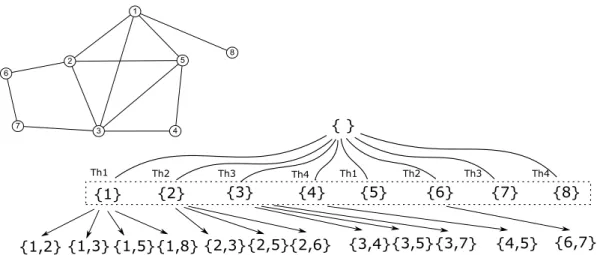
2.2.6. Enumeration tree based community detection

Many graph mining algorithms create an enumeration tree to mine communities or clusters in a

graph [81, 54, 71]. Figure 2.2 shows a sample graph and its enumeration tree. The enumeration tree starts

with a null set at the root. The first level search nodes in the enumeration tree contain each individual

vertex of the graph. Each of these first level search nodes are expanded to form children nodes by adding

one vertex from the graph, which is not already present in that search node. An enumeration tree typically

follows a strict ordering of vertices which makes sure that the same subgraph is not repeated twice in the

(21)

the other vertices already present in the search node. Each search node in the tree satisfies the community

definition. The clique definition for a community is an anti-monotone property [55], i.e., as we go down the

enumeration tree, if a search node doesn’t satisfy the clique definition then no child node generating from

that search node will ever satisfy the clique definition. Thus we can stop generating child nodes from that

search node. 1 3 2 4 {1,2} {1,3} {2,3} {1} {2} {3} {4} {1,4} {2,4}{3,4} {1,2,3} {1,2,4} {1,3,4} {2,3,4} {1,2,3,4} {} (a) (b)

Figure 2.2. Enumeration tree example. (a) A sample graph. (b) Enumeration tree for the sample graph; node order 1<2<3<4 is followed while generating child nodes.

2.2.6.1. Enumerating quasi cliques

Quick is an eﬃcient algorithm to find maximal quasi-cliques from an undirected graph discussed in

[54]. This algorithm builds an enumeration tree where each node in the tree has a candidate set of vertices

which can be used to extend the current search node. Quick follows a strict ordering among its vertices

to reduce the number of duplicate search node in its sample space. Quick applies several eﬀective pruning

techniques based on the degree of the vertices to prune unqualified vertices as early as possible, such as

pruning on the vertex degree and graph diameter.

2.2.6.2. Enumerating dense clusters

The algorithm discussed by Uno et al. [71], traverses the enumeration tree in a depth first manner.

This algorithm uses the reverse search technique [3] to generate child search nodes in the enumeration tree.

Reverse search does not need to memorize the previously visited search nodes to avoid duplicates. The

algorithm adapts the reverse search paradigm and only enumerates valid quasi clique child search nodes at

(22)

2.3. Cohesive community detection

2.3.1. Attributes in graphs

Often additional data sources are available which can annotate the nodes or the edges of the graph

with attribute data. In a PPI network an attribute value can represent gene expression data, which encodes

the diﬀerential expression value of each gene when exposed to stimuli. In a social network, an attribute might

correspond to the personal profile of a member such as age, interests, locale, etc. The concept of homophily

suggests that cultural, behavorial, genetic or material information that flows through a network tends to

get localized to people or entities with similar attributes [56]. So in addition to observing interactions in a

network, it is also important to consider the attributes of entities [36, 44].

2.3.2. Node attributes

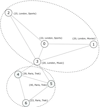
Node attributes represent properties of vertices in a graph. As noted above the profile data in a

social network such as age and interests are examples of node attributes. Usually they are modeled as a

vector of attributes corresponding to each vertex in the graph. Figure 2.3 shows a sample social network

where each node is a person and the attributes shown are properties of the person such as age, city and

interests. The figure shows two cohesive communities which are not only dense but also have similarity in

their attributes. Notice that each vertex is similar on a subset of attributes with the attributes of other

vertices in its community, for e.g., vertices (0,1,2,3) are similar in age and city.

0 ₁ 2 3 4 5 6 {20, London, Movies} {25, London, Sports} {22, London, Sports} {20, London, Music} {23, Paris, Trek} {39, Paris, Trek} {40, Paris, Trek}

(23)

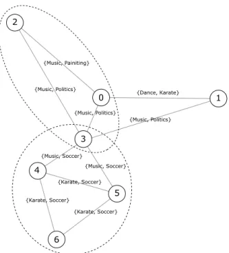
0 1 2 4 5 6 {Music, Painiting} {Music, Politics} {Music, Politics} {Music, Politics} {Dance, Karate} {Music, Soccer} {Music, Soccer} {Karate, Soccer} {Karate, Soccer} {Karate, Soccer} 3

Figure 2.4. Graph with edge attributes and two cohesive communities.

2.3.3. Edge attributes

Edges can have properties too and they are modeled as edge attributes. For example, in a social

network the length of the relationship measured in time between two friends is an attribute of their

rela-tionship. In a chemical network the strength of the bond between two molecules can be modeled as an edge

attribute. Edge attributes are typically modeled as a vector of attributes corresponding to each edge in

the graph. Figure 2.4 shows another sample social network with edge attributes. The attribute on a edge

shows the type of online activity between two people. Vertices (3,4,5,6) forms a community where all edges

have {soccer} as a common attribute. Edge-based content is much more challenging, because the diﬀerent interests of the same individual may be reflected in diﬀerent edges.

In an cohesive community detection approach, the communities are not only matched for graph

topology but also for attribute similarity. Many cohesive approaches combining graph topology data with

attribute data have been proposed. Some rely on full space clustering of attributes [67] while others consider

sub space clustering [36, 30, 18]. Full space clustering often leads to poor results in high dimensional dataset

because there is a high probability of some irrelevant attribute to obfuscate the cluster.

2.4. Enumeration algorithms for cohesive community detection

This section will briefly introduce some of the state of the art algorithms for mining cohesive

com-munities. All of these algorithms requires three parameters; a density thresholdγwhich controls the density of output modules, an attribute profile thresholdtand number of cohesive attributes thresholdsmin which together controls the cohesiveness of each module in the community

(24)

2.4.1. GAMer

The GAMer algorithm [36] proposed an enumeration approach which uses quasi-clique definition for

community or cluster density. GAMer integrates the community detection with vertex attribute sub space

clustering technique which identifies locally relevant (similar) subsets of attributes for each community. The

quasi clique definition and sub space clustering together form a cluster definition for GAMer. Quasi-clique

definition is not anti monotone, i.e., the quasi clique density of the subgraph cannot be used to prune the

search space in the enumeration tree. However attribute subspace clustering is an anti-monotone property;

if at any search node the number of similar attributes falls below a threshold, then the entire subtree rooted

at the current search node can be pruned.

2.4.2. DME

The quasi-clique density is a little restrictive as each vertex is still required to have a minimum

degree. Georgii et al. proposed the Dense Module Enumeration (DME) for weighted networks [30]. This

algorithm uses a relaxed definition of density which generates more clusters than GAMer. Similar to GAMer,

DME also builds an enumeration tree and outputs dense and cohesive clusters. The density definition used

in DME is not anti-monotone. However DME employs the reverse search technique [3] which traverses the

tree in a way such that the density property going down the enumeration tree is always decreasing.

2.4.3. DECOB

Like the above algorithms, the DECOB algorithm exhaustively finds maximal dense connected

biclusters [18]. DECOB starts with the cohesive or similar edges and adds a new neighbor vertex to each

edge. If the new pattern is dense and cohesive DECOB keeps it in a list otherwise discards it. Building this

way, the algorithm finds out all the dense and cohesive patterns that have 3 vertices (since it started from

an edge containing two vertices). The algorithm iteratively works on this list to find maximal dense and

cohesive patterns at each pattern size level. Unlike the GAMer and DME this algorithm walks the patterns

in Breadth First Search (BFS) manner while the two preceding algorithms walk the enumeration tree in

(25)

3. MINING DENSE COHESIVE SUBNETWORKS

In this chapter we look at the problem of mining dense and cohesive community or cluster. We

first establish the definition of our dense and cohesive cluster and later show our algorithm followed by the

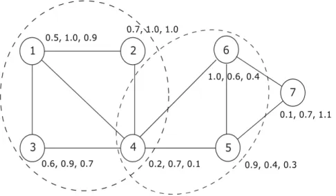
results. Figure 3.1 shows a graph with node attributes. The figure shows two communities which are both

dense and similar in their attributes.

1 2 3 4 5 6 4 7 .4, 0.3 0 0.1, 0.7, 1.1

Figure 3.1. Example node attribute graph. The graph shows two communities, vertex 4 belongs to both communities.

3.1. Problem description

In this section, we introduce some preliminary definitions that are used throughout the paper. We then describe the problem of mining maximal dense cohesive subgraphs.

Definition 1. A graph G= (V, E, f) is an undirected graph, where V ={v1, ..., vn} is the set of vertices, E ⊆ V ×V is the set of edges, and f : V → Rd is a function that maps a vertex to a d-dimensional real vector.

The number of vertices and number of edges in Gare denoted as|V|and |E|, respectively. We use thed-dimensional vector to represent the attributes associated with a vertex. The attributes of all vertices can be represented by an attribute matrixX∈ Rn×d, wherexij is the attribute value of the ith vertex in jth attribute. The ith row of the matrix X is the attribute vector of the ith

(26)

From figure 3.1; we have V ={1,2,3,4,5,6,7}, E={(1,2),(1,3),(1,4),(2,4),· · · ,(6,7)},

and f(v1) = (0.5,1.0,0.9)

For any subset U ⊆V, we denote G[U] = (U, E[U]) as the subgraph of G induced by U, i.e. E[U] is the set of edges ofGwhose endpoints are both inU.

We define thedensity property (denoted as ρ) of an induced subgraph G[U] as the ratio of the number of edges in the induced subgraph (E[U]) by the total possible edges inG[U]. In Figure 3.1, for U ={1,2,3,4},ρ(U) = 5/6 = 0.83.

ρ(G[U]) =ρ(U) = 2|E[U]| |U|(|U| −1)

Definition 2. Given a tolerance threshold t and a set of vertices U; where each vertex has d dimensional vector representing attributes. The kth attribute is considered a cohesive attribute for vertices inU if the kth attribute values for all vertices in U diﬀer by at mostt.

∀ui, uj ∈U :|f(ui)[k]−f(uj)[k]| ≤t

For a threshold t, let A(U, t) denotes the set of cohesive attributes, for simplicity we refer toA(U, t) as A(U) :

A(U) ={k1, k2,· · ·, kl},1≤ki≤d

In Figure 3.1, for U = {4,5,6} and t = 0.3, A(U) = {2,3} since the three vertices have ‘similar’ values in the 2nd and 3rd attributes, i.e. the maximum diﬀerence between the attribute values for the three vertices inU for each of the 2nd and 3rd attribute is less than or equal tot. Definition 3. Given a tolerance thresholdt, a dimensionality threshold smin, an induced subgraph G[U]is said to be acohesive subgraphif the cardinality of the set of cohesive attributes is at least smin, i.e. |A(U)| ≥smin

The dimensionality threshold smin is the minimum number of ‘similar’ attributes a set of vertices must have in order to form a cohesive subgraph. In Figure 3.1, for t= 0.3 and smin = 2, the subgraph induced by U ={4,5,6} is a cohesive subgraph.

(27)

Definition 4. Given a density threshold θ, an attribute tolerance thresholdt and a dimensionality threshold smin: G[U]is a dense cohesive subgraph if it satisfies the following conditions.

1. Density of the subgraph G[U] is atleast equal to the density threshold, ρ(U)≥θ.

2. The number of relevant attributes should be at-least equal to dimensionality threshold, i.e.

|A(U)| ≥smin from definition 3

We can see from figure 3.1 that the subgraph induced by U = {1, 2, 4} vertices is both dense and cohesive. ρ(U) = 3₃ = 1 and vertices in U have similar values in 1st and 2nd attributes fort= 0.5.

According to Definition 4, a dense cohesive subgraph is any subgraph that can satisfy the density condition and has cohesive set of attributes. However, a single vertex is dense by definition and has absolute similarity among its own attributes. Also, a cluster of two vertices with a single edge has a density of 1. It only needs to satisfy the second condition of definition 4 in order to be considered a cohesive subgraph. It is obvious that we need a way to keep these kinds of unmeaningful subgraphs out of our result set. A common solution is to mine for the maximal

subgraphs. A subgraph is considered maximal if it has no direct superset which is cohesive and satisfies the density threshold condition. In this way we will not output every possible sub graph like{1, 2, 4}and {1, 3, 4} which are subsumed in the maximal cluster{1, 2, 3, 4} from figure 3.1 Definition 5. A cohesive dense subgraph induced byU ismaximalif no superset U′⊇U is dense and cohesive.

Problem Definition: Given an attributed graphG= (V, E, f), three thresholdsθ, t, smin,

the problem of mining the set ofmaximal dense cohesive subgraphs is to find the set: P ={U1, U2, U3,· · · , U_|P|}

such that everyUi ∈ Pis a maximal dense cohesive subgraph. EachUiis a tuple{Gi, Ai}containing a subgraph and its relevant attributes.

(28)

3.2. Algorithm

3.2.1. RedCone approach

In this section we introduce our algorithm for mining REpresentative Dense COhesive subNEtworks (RedCone). As the name suggests, the algorithm discovers maximal dense cohesive clusters in a graph. It later tries to find representative clusters for all such cohesive dense clusters.

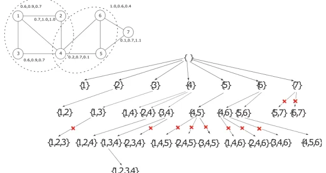
{ } {1} {2} {3} {4} {5} {6} {7} { 1,2} {1,3} {1,4}{2,4} {3,4} {1,2,3} {1,2,4} {1,3,4}{2,3,4} {1,4,5} {1,2,3,4} {4,5} {4,6}{5,6} {5,7} {6,7} {2,4,5}{3,4,5} {1,4,6}{2,4,6}{3,4,6} {4,5,6} 1 2 3 4 5 6 4 7 0.6,0.9,0.7 0.6,0.9,0.7 0.7,1.0,1.0 0.2,0.7,0.1 1.0,0.6,0.4 0.1,0.7,1.1

Figure 3.2. Example graph (a) and its enumeration tree (b). θ = 0.7. Crosses show which branches are pruned. The discovered maximal clusters are in green.

We adapt the cluster enumeration approach as described in DME [30]. The cluster enumer-ation approach starts with an empty set and then iteratively grows into larger sets by adding one vertex at a time. The algorithm builds an enumeration tree (Figure 3.2) where each search node represents a dense cohesive cluster. Even though the density constraint is not anti-monotone, the reverse search technique [3] traverses the tree in a way such that the density property going down the enumeration tree is always decreasing while the node size is increasing. This is achieved by following a strict definition of parent-child relationship in the enumeration tree [30]. Essentially at every given search node all possible child search nodes are generated and only valid child search nodes are explored. The valid child search nodes maintain the density monotonicity property and

(29)

Algorithm 1 Maximal Dense Cohesive Cluster Discovery

Input:

G= (V, E, f): an attributed graph

min size: the minimum size of cluster to include in results

θ: density threshold

t: tolerance threshold between two attribute values in a single subspace

smin: minimum number of similar attributes per cluster

Output:

P: maximal cohesive clusters

1: Remove all non cohesive edges from input graph

2: P={}

3: _{MineDenseclusters}({})

4: functionMineDenseclusters(U) 5: locally maximal←true

6: forv∈V\U do 7: LetU′=U∪v

8: if ρ(U′)≥θand|A(U′)| ≥sminthen 9: locally maximal←f alse

10: if isChild(U′,U)then

11: MineDenseclusters(U′)

12: end if

13: end if

14: end for

15: if locally maximaland|U| ≥min sizethen 16: P=P ∪U

17: end if 18: end function 19: returnP

also follow a strict ordering which ensures that each search node will be visited only once. A func-tion ord defines a strict total ordering on the nodes, i.e. for each node pairu,v withu̸=v either

ord(u) > ord(v) orord(u) < ord(v) holds. With this, the parent-child relationship for modules is defined as follows. Given U and v∈V \U. U∗ :=U∪v is a child ofU if and only if

∀u∈U : (degU∗(v)< degU∗(u))∨(degU∗(v) =degU∗(u)∧ord(v)< ord(u))

Here (degU∗(v) stands for the degree of vertex v in the subgraph induced by U∗. We obtain the

parent of a module by removing the smallest ordered vertex with the least degree.

Algorithm 6 shows the pseudo code for our cluster discovery process. The recursive function builds an enumeration tree like the example in figure 3.2. Note that we only consider search node expansion if the conditions given in definition 4 are met (line 16). If a cluster doesn’t have a cohesive and dense superset then that cluster by definition 5 is maximally dense and cohesive. The result of this algorithm is the set of maximal dense cohesive clustersP. From figure 3.1 one can observe that

(30)

there are two maximal dense cohesive clusters {1,2,3,4} and {4,5,6} which are similar in atleast 2 attributes. Figure 3.2 demonstrates how our algorithm arrives at these two clusters.

We employ diﬀerent pruning strategies to avoid visiting branches that will not result in cohesive clusters. The algorithm starts by removing edges from the input graph which are not cohesive according to definition 3. Due to the anti-monotonicity of the cohesive constraint, pruning an edge will not result in missing any clusters because the pair of vertices (end points) cannot be together in any cohesive cluster. In figure 3.2 (a) the edge between vertices 5 and 7 is not cohesive in two attributes for t= 0.6, therefore we can remove that edge from the graph without missing any clusters.

The second pruning is based on reverse search enumeration. Since the reverse search prin-ciple guarantees that the search nodes are grown in a decreasing order of density, we can safely assume that if any search node does not meet the density threshold, θ, then we can prune that search node. This helps by eliminating the entire subtree from the search space.

Before a new child search node can be created, the algorithm checks to see if the potential child search node is cohesive. If it is cohesive then the algorithm creates the child node and recursively extends it. However if no cohesive dense child node exists for the current search node then the current search node is maximally cohesive and it can be added to P (line 24). Both of these two pruning strategies are enforced in line 16 of algorithm 6.

3.2.2. Multithreaded RedCone

Recall that RedCone requires density and profile thresholds to reduce the search space of the input graph. For relaxed constraints, the search space is huge which in turn takes a very long time to enumerate all qualifying clusters. For reference, RedCone , DME, Gamer and DECOB algorithms took multiple days to completely enumerate all clusters in the BioGRID dataset, which has 6249 vertices and 224,587 edges. The result set (output space) contained several million clusters which qualified a very relaxed input constraints on density and cohesive profile. As this example shows the above algorithms including RedCone don’t scale very well for even a modestly sized input graph or as constraints are further relaxed.

In this section we propose a multithreaded implementation for RedCone , called MT Redcone to address the issues of scale.

(31)

1 2 3 5 8 6 4 7 { } {1} {2} {3} {4} {5} {6} {7} {8} Th1 Th2 Th3 Th4 Th1 Th2 Th3 Th4 {1,2} {1,3} {1,5}{1,8} {2,3}{2,5}{2,6} {3,4}{3,5}{3,7} {4,5} {6,7}

Figure 3.3. The input graph and its corresponding enumeration tree. There are four threads which build the enumeration tree independently. There are 4 threads and each thread builds subtree for 2 first level children.

RedCone mines maximal dense cohesive subgraphs by following a reverse search enumeration technique [3]. The reverse search technique guarantees that the enumeration of child search node is only dependent on its parent search node and is independent of any shared structure. This property can be exploited to parallelize the enumeration tree traversal.

Figure 3.3 shows an example of the enumeration tree that created by MT Redcone for the input graph shown in figure 3.1. Utilizing the reverse search principle, the subtrees rooted under each first level node in the enumeration tree can be enumerated independently. This suggests that we can spawn multiple threads at the root, and each thread creates the sub tree under each of the first level nodes. Algorithm 3.2.2 shows the psuedo code for MT Redcone . Apart from the usual inputs such as graph G, density threshold θ, tolerance threshold t and dimensionality threshold

smin, MT Redcone also requires a number of threads input numthreads. The algorithm begins by spawning the requested number of threads (line 3). Each thread then iterates over the first level nodes, selects a vertex and traverses its enumeration subtree (line 9). The output of this algorithm P is a list of maximal cohesive dense clusters.

3.3. Representative Set

The number of maximal dense cohesive clusters can be astronomically large, depending on the density and cohesive constraints. Moreover, these clusters have overlap in both the vertices and their relevant attributes. For analysis, often a summarized set of all the reported clusters is desired. This set should be representative of the reported clusters such that all the clusters not

(32)

Algorithm 2 Multi-threaded Maximal Dense Cohesive Cluster Discovery

Input:

G= (V, E, f): an attributed graph

min size: the minimum size of cluster to include in results

θ: density threshold

t: tolerance threshold between two attribute values in a single subspace

smin: minimum number of similar attributes per cluster

numthreads: Number of threads to spawn for parallel execution

Output:

P: maximal cohesive clusters

1: Remove all non cohesive edges from input graph

2: P={}

3: threads[] =spawn threads(numthreads) 4: start all threads(threads[], T hreadStart) 5: join all threads(threads[])

6: function_ThreadStart 7: forv∈V do

8: execute thread(t,_Mineclusters(v)) 9: end for

10: end function 11: _Mineclusters({})

12: functionMineclusters(U) 13: locally maximal←true

14: forv∈V\U do 15: LetU′=U∪v

16: if ρ(U′)≥θand|A(U′)| ≥sminthen 17: locally maximal←f alse

18: if _isChild(U′,U)then

19: Mineclusters(U′)

20: end if

21: end if

22: end for

23: if locally maximaland|U| ≥min sizethen 24: P=P ∪U

25: end if 26: end function 27: returnP

in the representative set should have at least one ‘similar’ cluster in the representative set. We propose an approach for selecting a representative set of clusters for the maximal cohesive clusters. 3.3.1. Finding Similarity Scores

In the first step, we introduce a similarity measure to quantify the similarity between two maximal dense cohesive clusters and calculate the similarity scores between all pairs of the reported clusters.

Given two clusterU,U′, letSU U′ denotes the Jaccard similarity coeﬃcient between the sets of vertices of the two clusters.

S_{U U}v ′ = |U ∩U

′_|

(33)

The relevant attribute similarity between the two clusters is captured by the Jaccard simi-larity coeﬃcient between the sets of relevant attributes.

S_{U U}a ′ = |A(U)∩A(U

′)_|

|A(U)∪A(U′)| (3.2)

We define the cluster similarity as linear combination of the vertices and relevant attribute similarities as shown below, where α is a user-defined parameter (0 ≤ α ≤ 1) to control the contribution of the vertices similarity to the pair wise cluster similarity.

SU U′ =α∗SU Uv ′+ (1−α)∗SU Ua ′ (3.3) 3 1 2 3 1 2 4 {1,2} 5 1 4 {1,2,3,4} P1 P2 P3 5 1 3 {2,3,4,5} P4 4 5 1 3 {2,3,4} P5 4 2 0.41 0.33 0.55 0.58 0.6 0.375 0.775 0.55 P1 P3 P4 P5 P2 P1 P3 P4 P5 P2 6 6 0.775 0.3 (a) (b) (c) k-medoids 0.59 0.67 0.45 0.52 0.4 0.625 0.225 0.45 0.225 0.7 {2,3} Relevant Attributes

Figure 3.4. Finding representative clusters. (a) The maximal cohesive clusters. (b) The cluster similarity graph for α = 0.5, edges show dissimilarity between clusters; (c) Applying k-medoids algorithm results in finding clusters and medoids (highlighted in blue), edges show distances between clusters.

The cluster similarity between the first two clusters shown in Figure 3.4(a) is calculated as follows (for alpha=0.5):

SP1P2 = 0.5∗ 2

6 + 0.5∗ 1

(34)

The two clusters share two vertices out of the six vertices and one relevant attribute out of the three relevant attributes.

3.3.2. Similarity Graph

The cluster similarity graph represents the result clusters as nodes and its similarity as distance on the edges to other nodes. More formally, we construct the cluster similarity graph

GP = (VP, EP), whereVP ={U1, U2,· · · , Uk} represent the set of maximal dense cohesive clusters

and there is an edge between two vertices in this graph where the distance of edge (ui, uj) isSUiUj.

Figure 3.4(a) shows 5 clusters and Figure 3.4(b) shows the cluster similarity of these 5 clusters. Each node in cluster similarity graph is a subgraph as shown in 3.4(a) and edge weights represent the similarities between clusters. The similarities range from 0 to 1, with 0 similarity score indicating no overlap in both the vertices and the relevant attributes and 1 indicating complete overlap.

3.3.3. Representative clusters - Set cover approach

The problem of selecting representative clusters from a large set of result clusters has been previously studied in [9]. In that paper finding the representative clusters problem was mapped to the problem of finding the dominating set of minimum size from the similarity graph. Given the undirected similarity graph GP = (VP, EP), the problem of selecting the smallest dominating set

is to select the smallest set of nodes (clusters) S ⊆Vp such that every node not in S is connected

to at least one node in S.

3.3.4. Representative clusters - K-Medoids approach

The problem of selecting representative clusters can be mapped to the problem of finding

k medoids from multiple observations using the k-medoids algorithm. k-medoids is a classical partitioning technique that clusters the data set of nnodes into k clusters. Each of these clusters have a center or medoid. A medoid can be defined as the node of a cluster whose average distance to all the nodes in the cluster is minimal, i.e., it is the most centrally located node in the cluster. The objective of this algorithm is to partition all the n nodes into k clusters such that average distance of all the nodes in each cluster from its corresponding medoid is minimized. As a by product the algorithm finds k medoids (nodes) which are most centrally located within their own clusters in the graph. Given an undirected similarity graphGP = (VP, EP), the problem of finding representative result nodes is to find thek medoids of that graph.

(35)

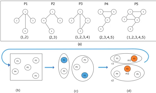
Figure 3.5 shows the modified K-medoids algorithm in action with a few output maximal cohesive dense clusters{p1, p2, ..., p5}. Figure 3.5 (a) shows the network structure of these maximal

cohesive dense clusters and also lists the cohesive attributes of each cluster below. These cohesive clusters are projected as points in space andK random points are selected as medoids. This process is shown in figure 3.5 (b).

After the random selection of points, the modified K-Medoids algorithm detects partitions around these random medoids as shown in figure 3.5 (c). After detecting the partitions, new medoids are again determined for each partition as shown in figure 3.5 (d). This process repeats itself by finding new partition again around the new medoids. Finally this process stops when a steady state is reached, i.e, new medoids are exactly same as the previous medoids. The final medoids at the steady state are the representative maximal cohesive dense clusters.

3 1 2 3 1 2 4 (1,2) 5 1 4 (1,2,3,4) (2,3) P1 P2 P3 5 1 3 (2,3,4,5) P4 4 5 1 3 (1,2,3,4,5) P5 4 2 (a) 6 6 (c) (b) (d) P1 P3 P4 P5 P2 P1 P3 P4 P5 P2 P1 P3 P4 P5 P2 c1 c2 m1 m2

Figure 3.5. Representative clusters. (a) Set of maximal cohesive dense clusters, (b) Projecting maximal cohesive dense clusters to points in space. (c) Finding partitions around the random medoids. (d) Detecting steady state medoids m1 =P3 and m2 =P2 and its partitions c1 and c2 respectively. The representative maximal cohesive dense clusters are the set of steady state medoids

m1, m2

This modified K-Medoids algorithm, distributes a given set of points {p1, p2, ..., pn}intoK

(36)

partitionc which can be represented as k ∑ i=1 ∑ y∈ci Symi

where mi represent the medoids and S represents the similarity between two maximal cohesive dense cluster.

Now we shall define some metrics to understand the quality of these output medoids (rep-resentative clusters) as produced by the K-Medoids algorithm.

Definition 6. Given a set of points {p1, p2, ..., pn}, k partitions {c1, c2, ..., ck} and their respective medoids {m1, m2, ..., mk}, the average intra partition similarity is defined as average sum of the similarities of each point p∈cx to their corresponding medoid mx.

AvgP artitionSim= ( k ∑ i=1 ∑ y∈ci Symi)/|{p1, p2, ..., pn}|

The AvgP artitionSim similarity captures the quality of all partitions. A high value indi-cates that each medoid is centrally located in its partition, and, has high similarity with all other points in the partition. A low value indicates that the medoid is not equally similar to all other points in its partition, suggesting poor partitioning.

Definition 7. Given a set of points {p1, p2, ..., pn}, k partitions {c1, c2, ..., ck} and their respective medoids {m1, m2, ..., mk}, the average inter medoid similarity is defined as average of sum of the pair wise similarities between the set of medoids.

AvgM edoidSim= ( k ∑ i=1 k ∑ j=i+1 Smimj)/(M∗(M −1)/2) where M =|{m1, m2, ..., mk}|

As opposed to the AvgP artitionSim, AvgM edoidSim indicates the dissimilarity between the detected medoids. If the medoids are suﬃciently similar to all points in their partition than they should be dissimilar to other medoids. In high quality partitions, we expect a high value for

(37)

In this perspective these two similarities complement each other. We report our findings on repre-sentative sets using these metrics.

Finally, the runtime of K-Medoids isO(K∗n∗iter) +O(K2∗iter) whereiterrepresents the number of iterations to reach to steady state andKrepresents the desired number of representative clusters. Since both K and iter are compile time constants, K-Medoids is better when compared to set cover algorithm mentioned in section 3.3.3 which took O(n2).

3.4. Experiments

We compare our algorithm against GAMer [36] and DECOB [18] using two real-world net-works and their associated attribute data: High Confidence Yeast (YeastHC)[37] and theBioGRID

[11]. All experiments were run independently on an Arch Linux operating system with an Intel Core i5-2500K (3.3GHz) processor and 8 Gigabytes of main memory.

3.4.1. Cohesive clusters in YeastHC

For this dataset, we represent the yeast interaction network as a graph and gene profile data as attributes. The interaction network contains 4,008 vertices and 9,857 edges in its graph. We include gene profile information which denotes the diﬀerential expression value of each gene when exposed to 173 diﬀerent experiments [29]. We used real (floating point) attribute values and varied the attribute tolerance thresholdtin increments of 0.1.

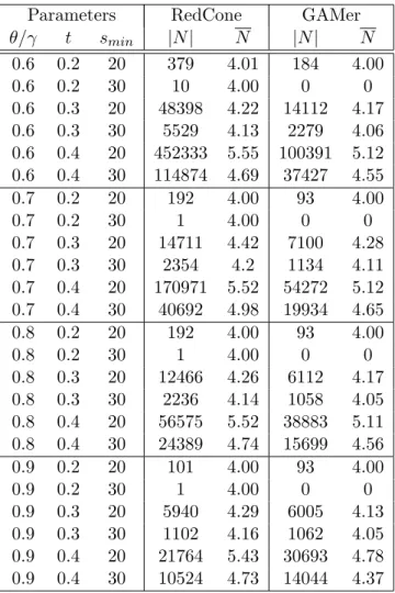
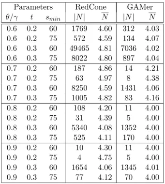
Table 3.1 compares the topological properties reported by RedCone and GAMer for this dataset. In the table, |N|denotes the number of resulting clusters and N represents the average size. RedCone reports notably higher number of these clusters because it has a relaxed density constraint and also because GAMer reports summarized modules. The average cluster size reported by RedCone is also high for higher tolerance thresholds which can be again attributed to its relaxed density constraint. Since DECOB reports the same results as RedCone we only compare against DECOB for the running time.

We also performed biological enrichment analysis using the Database for Annotation, Visualization, and Integrated Discovery — DAVID [41, 42] on the YeastHC dataset. In order to verify the significance of our results, we attempted to find enrichment of Gene Ontology process terms (GOTERMS) as well as KEGG pathway enrichment in our resulting clusters.

Figure 3.6 plots the resulting clusters listed by RedCone with the percentage of modules enriched in GOTERMs and KEGG pathways. As we can see for densities 0.7 to 0.9 almost all

(38)

Table 3.1. Topological properties of cohesive dense clusters for Yeast dataset.

Parameters RedCone GAMer

θ/γ t smin |N| N |N| N 0.6 0.2 20 379 4.01 184 4.00 0.6 0.2 30 10 4.00 0 0 0.6 0.3 20 48398 4.22 14112 4.17 0.6 0.3 30 5529 4.13 2279 4.06 0.6 0.4 20 452333 5.55 100391 5.12 0.6 0.4 30 114874 4.69 37427 4.55 0.7 0.2 20 192 4.00 93 4.00 0.7 0.2 30 1 4.00 0 0 0.7 0.3 20 14711 4.42 7100 4.28 0.7 0.3 30 2354 4.2 1134 4.11 0.7 0.4 20 170971 5.52 54272 5.12 0.7 0.4 30 40692 4.98 19934 4.65 0.8 0.2 20 192 4.00 93 4.00 0.8 0.2 30 1 4.00 0 0 0.8 0.3 20 12466 4.26 6112 4.17 0.8 0.3 30 2236 4.14 1058 4.05 0.8 0.4 20 56575 5.52 38883 5.11 0.8 0.4 30 24389 4.74 15699 4.56 0.9 0.2 20 101 4.00 93 4.00 0.9 0.2 30 1 4.00 0 0 0.9 0.3 20 5940 4.29 6005 4.13 0.9 0.3 30 1102 4.16 1062 4.05 0.9 0.4 20 21764 5.43 30693 4.78 0.9 0.4 30 10524 4.73 14044 4.37

resulting clusters are enriched in GOTERMs. As density goes down RedCone outputs very large number of clusters because of relaxed density constraint, hence not all clusters are enriched.

Figure 3.7 shows two maximal clusters from the RedCone’s output on the YeastHC dataset and two matrices illustrating the attribute data for the vertices in the two clusters. The matrix shows the vertices on the rows and attributes on the columns. The first 20 columns in the matrix are the attributes where these vertices are similar and therefore show very little deviation in its gray shade. The last 20 columns are a sample of 20 attributes from the remaining 153 attributes, where these vertices are not similar. This similarity is evident by the homogenity of gray shade in the first 20 columns versus variation of gray shade in the last 20 columns. This image is helpful in understanding that the output clusters are not only dense in the graph structure but they also have similar values in a number of attributes.