Two-Stream Convolutional Networks for Dynamic Texture Synthesis

(1)

Two-Stream Convolutional Networks for Dynamic

Texture Synthesis

MATTHEW TESFALDET

A THESIS SUBMITTED TO

THE FACULTY OF GRADUATE STUDIES

IN PARTIAL FULFILLMENT OF THE REQUIREMENTS FOR THE DEGREE OF

MASTER OF SCIENCE

GRADUATE PROGRAM IN COMPUTER SCIENCE YORK UNIVERSITY

TORONTO, ONTARIO August, 2018

(2)

Abstract

This thesis introduces a two-stream model for dynamic texture synthesis. The model is based on pre-trained convolutional networks (ConvNets) that target two independent tasks: (i) object recognition, and (ii) optical flow regression. Given an input dynamic texture, statistics of filter responses from the object recognition and optical flow ConvNets encapsulate the per-frame appearance and dynamics of the input texture, respectively. To synthesize a dynamic texture, a randomly initial-ized input sequence is optiminitial-ized to match the feature statistics from each stream of an example texture. In addition, the synthesis approach is applied to combine the texture appearance from one texture with the dynamics of another to generate entirely novel dynamic textures. Overall, the proposed approach generates high quality samples that match both the framewise appearance and temporal evolu-tion of input texture. Finally, a quantitative evaluaevolu-tion of the proposed dynamic texture synthesis approach is performed via a large-scale user study.

(3)

Acknowledgements

First and foremost, I am grateful to my parents, Bereket and Simret Tesfaldet, for their unending commitment to my well-being and utmost support during trying moments of my research.

I am thankful to my mentors and supervisors, Marcus Brubaker and Kosta Derpanis, for their support and patience in guiding me these past two years. I am also thankful for the many opportunities they have given me for engaging with the vibrant community of computer vision and deep learning researchers and practitioners. I look forward to continuing my research with them.

I am grateful to Rick Wildes and Michael Brown for the many fruitful and en-joyable discussions we have had about research during my time at York University. I thank Rick for his comments and suggestions regarding the thesis manuscript.

I acknowledge the financial support of the Canadian Graduate Scholarship (CGS) awarded by the Natural Sciences and Engineering Research Council of Canada (NSERC). This research was undertaken as part of the Vision: Science to Applications program, thanks in part to funding from the Canada First Research Excellence Fund.

I reserve an additional, special thanks to Kosta Derpanis for his personal and academic support over the past five years, and for introducing me to the wonderful world of computer vision and deep learning. Your inspiring commitment to the success of your students, both in the classroom and in the lab, has helped this “young padawan” take a large step towards realizing his goals.

(4)

List of Tables

A.1 Per-texture accuracies using the concatenation layer . . . 94 A.2 Per-texture accuracies averaged over a range of exposure times,

us-ing the concatenation layer . . . 95 A.3 Per-texture accuracies using the flow decode layer . . . 96 A.4 Per-texture accuracies averaged over a range of exposure times,

us-ing the flow decode layer . . . 97 A.5 Accuracies of textures grouped by appearances, using the

concate-nation layer . . . 98 A.6 Accuracies of textures grouped by appearances, averaged over a

range of exposure times, using the concatenation layer . . . 98 A.7 Accuracies of textures grouped by appearances, using the flow

de-code layer . . . 98 A.8 Accuracies of textures grouped by appearances, averaged over a

range of exposure times, using the flow decode layer . . . 98 A.9 Accuracies of textures grouped by dynamics, using the

concatena-tion layer . . . 99 A.10 Accuracies of textures grouped by dynamics, averaged over a range

of exposure times, using the concatenation layer . . . 99 A.11 Accuracies of textures grouped by dynamics, using the flow decode

layer . . . 99 A.12 Accuracies of textures grouped by dynamics, averaged over a range

of exposure times, using the flow decode layer . . . 99 A.13 Average accuracy over all textures, using the concatenation layer . . 100

(8)

A.14 Average accuracy over all textures, averaged over a range of expo-sure times, using the concatenation layer . . . 100 A.15 Average accuracy over all textures, using the flow decode layer . . . 100 A.16 Average accuracy over all textures, averaged over a range of

(9)

List of Figures

1.1 Definition of a static texture . . . 2

1.2 Texture synthesis . . . 3

1.3 Image style transfer . . . 4

1.4 Dynamic texture synthesis and dynamics style transfer . . . 6

2.1 Static texture synthesis with a convolutional network . . . 18

2.2 Computing the Gram matrix from activation maps . . . 19

2.3 Dynamics representation spectrum . . . 23

2.4 Optical flow visualization . . . 24

2.5 Spacetime texture spectrum . . . 27

3.1 Two-stream dynamic texture generation . . . 31

3.2 Dynamics stream ConvNet . . . 38

3.3 Learned spatiotemporal filters in the first layer of the dynamics stream 41 3.4 Incremental texture synthesis. . . 45

4.1 Dynamic texture synthesis success examples . . . 50

4.2 Dynamic texture synthesis success examples . . . 51

4.3 Dynamic texture synthesis failure examples . . . 53

4.4 Two-stream dynamic texture synthesis versus dynamics-only and appearance-only texture synthesis . . . 55

4.5 Temporally-endless texture synthesis . . . 56

4.6 Dynamics style transfer with incompatible appearance and dynam-ics targets . . . 57

(10)

4.8 Comparison with a dynamic texture synthesized using optical-flow directly . . . 60 4.9 Time-limited pairwise comparisons across all textures . . . 61 4.10 Time-limited pairwise comparisons across all textures, grouped by

appearance and dynamics . . . 63 4.11 Qualitative comparison with Funke et al.’s [20] model . . . 65 4.12 Qualitative comparison with Funke et al.’s [20] and Xie et al.’s [67]

model . . . 67 A.1 Example of a sentinel dynamic texture for the user study . . . 88 A.2 Per-texture accuracies averaged over exposure times . . . 93

(11)

Chapter 1 Introduction

1.1 Motivation

The natural world is rich in visual texture. While a precise definition of texture remains to be found, most research consider it as visual patterns that exhibit local variations while maintaining global homogeneity, as shown in Fig. 1.1.

Textures can be static or dynamic: static textures exist in two-dimensional

(2D) image space (e.g., grass and water) while dynamic textures extend the

no-tion across time (e.g., fluttering grass and wavy water). As a result, local spatial

variations and global homogeneity extend across space and time. These

tem-poral patterns have previously been studied under a variety of names, including turbulent flow [32] (for extracting optical flow from fluids undergoing irregular fluctuations), temporal textures [47] (for recognition of moving patterns such as windblown trees or rippling water), time-varying textures [5] (for synthesizing stochastically-moving patterns), dynamic textures [13] (for modelling and synthe-sizing stochastically-moving patterns), textured motion [64] (for modelling and

(12)

Figure 1.1: Definition of a static texture. A static texture is a visual pattern that exhibits local spatial variations while maintaining global homogeneity. Observ-ing small apertures across the texture should reveal visual content that appears roughly the same, captured as feature statistics.

synthesizing patterns undergoing stochastic or consistent motion), and spacetime textures [12] (for classifying dynamic patterns). In this thesis, the term “dynamic texture” is adopted.

Both static and dynamic texture cues play important roles in our perception of surfaces. Understanding and characterizing these patterns has long been a problem of interest in human perception, computer vision, and computer graphics. In computer vision, studying the underlying statistics of textures allows us to gain insight as to how these complex structures can be interpreted and how we may be able to leverage this knowledge to inform certain vision-related tasks. Examples of such tasks include shape-from-texture [25], material recognition [10, 2], texture synthesis [31], and more recently, image style transfer [22]. In terms of specific applications, there are many in the creative-industry including, but not limited to, computer-generated imagery, digital painting, and image editing.

Shape-from-texture involves recovering the three-dimensional (3D) shape of an object from a 2D image by using texture as a cue. Gibson [25] proposed thetexture gradient as the primary basis of surface perception by humans. He conjectured that neighbouring areas on a textured surface are perceived diﬀerently only due

(13)

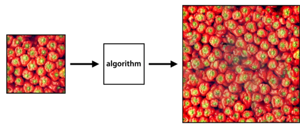
algorithm

Figure 1.2: Texture synthesis is the process of algorithmically constructing a tex-ture (right) that matches or extends a given source textex-ture (left) by taking advan-tage of its structural content.

to diﬀerences in surface orientation and distance from the observer.

Material recognition in computer vision involves recognizing material categories

(e.g., fabric, water, and wood) from an image based on the visual appearance

of surfaces. The visual appearance of a surface depends on several factors [10, 2], such as illumination, geometric structure at various scales, viewing direction, and surface reflectance properties,e.g., the Bidirectional Reflectance Distribution Function (BRDF) [46]. Notably, texture can be useful for distinguishing materials. For example, wood and water each have unique texture that easily distinguishes

the two. Dana et al. [10] introduced the Bidirectional Texture Function (BTF)

and demonstrated that the visual appearance of materials can be characterized by measuring texture.

Texture synthesis (Fig. 1.2) is the process of algorithmically constructing a texture that matches or extends a given source texture by taking advantage of its structural content. Heeger and Bergen [31] took advantage of the fact that two textures are often diﬃcult to discriminate when they produce a similar distribution of responses from a bank of linear filters. They used a combination of Laplacian and

(14)

Content

Style

Output

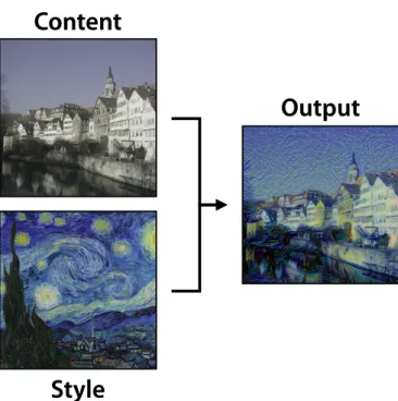
Figure 1.3: Image style transfer. The goal is to synthesize a texture (right) from an input “style” image (bottom-left) while constraining the process in order to preserve the semantic content of an input “content” image (top-left).

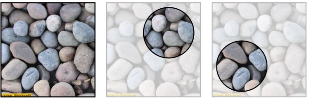
steerable pyramids to deconstruct a given texture and synthesized a new texture by matching the distributions of responses from each pyramid level. Portilla and Simoncelli [50] extended this approach by including complex “analytical” filters that allowed them to utilize measures of local phase and energy in their texture descriptors. More recently, Gatys et al. [21] demonstrated impressive results for texture synthesis by using a convolutional network (ConvNet) instead of a linear bank of filters to model the non-linear spatial statistics of a given texture.

Image style transfer (Fig. 1.3) is a recent technique where the goal is to

re-compose an image in the “style” (e.g., texture) of another image. This can be

considered as a texture transfer problem, as previously demonstrated by Efros et

al. [15], where they transferred a given texture to another image by stitching to-gether small patches of the given texture while conforming to the luminance of the

(15)

other image. Although the simplicity of their approach was attractive, it failed for highly structured textures due to patch boundary inconsistencies, limiting the selection of acceptable textures. Gatys et al. [21] modified their previous Con-vNet for texture synthesis to support texture transfer by including an additional objective that enforced the synthesized texture to match the semantic content of a given image, resulting in an image style transfer [22]. Unlike the patch-based method of Efros et al. [15], Gatys et al.’s approach of using a ConvNet was more robust to textures with long-range consistencies.

Motivated by the ConvNet model of Gatyset al. [21] for texture synthesis, the focus of this thesis is on the synthesis of dynamic texture samples, as captured in video, based on a single exemplar through the use of ConvNets. Inspired by Gatyset al.’s [22] method of image style transfer, a novel form of style transfer for dynamic textures is presented as well.

1.2 Summary of thesis

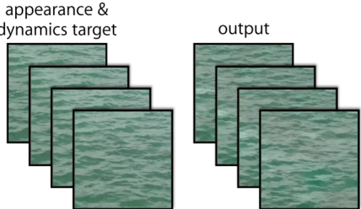
Many common dynamic textures are naturally described by the ensemble of ap-pearance and dynamics (i.e., spatial and temporal pattern variation) of their con-stituent elements. In this thesis, a factored analysis of dynamic textures in terms of their appearance and dynamics is proposed. This factored analysis is then used to enable dynamic texture synthesis based on an example dynamic texture as in-put. It also enables a novel form of style transfer where the target appearance and dynamics can be taken from diﬀerent sources—termeddynamics style transfer. An overview of dynamic texture synthesis and dynamics style transfer is shown in Fig. 1.4.

(16)

appearance &

dynamics target output

Dynamic Texture Synthesis

appearance target

output

dynamics target

Dynamics Style Transfer

Figure 1.4: Dynamic texture synthesis and dynamics style transfer. (top) Given an input dynamic texture as the target, the two-stream model synthesizes a novel dynamic texture that preserves the target’s appearance and dynamics character-istics. (bottom) The two-stream approach enables synthesis that combines the texture appearance from one target with the dynamics from another, resulting in a composition of the two.

(17)

The proposed model is constructed from two ConvNets: an appearance stream and a dynamics stream, which have been pre-trained for object recognition and optical flow regression, respectively. Similar to previous work on spatial textures [21, 31, 50], an input dynamic texture is summarized in terms of a set of spa-tiotemporal statistics of filter outputs from each stream. The appearance stream models the per-frame appearance of the input texture, while the dynamics stream models its temporal dynamics. The synthesis process consists of optimizing a ran-domly initialized noise pattern such that its spatiotemporal statistics from each stream match those of the input texture. The architecture is inspired by insights from human perception and neuroscience. In particular, psychophysical studies [9] show that humans are able to perceive the structure of a dynamic texture even in the absence of appearance cues, suggesting that the two streams are eﬀ ec-tively independent. Similarly, the two-stream hypothesis [26] models the human visual cortex in terms of two pathways, the ventral stream (involved with object recognition) and the dorsal stream (involved with motion processing). Two-stream networks have also been used for video understanding tasks in computer vision, with particular attention to action recognition [57, 18].

In this thesis, the two-stream analysis of dynamic textures is applied to texture synthesis. A range of dynamic textures are considered and it is demonstrated that the proposed approach generates novel, high quality samples that match both the frame-wise appearance and temporal evolution of an input example. Further, as stated previously, the factorization of appearance and dynamics enables a novel form of style transfer, where the dynamics of one texture are combined with the appearance of a diﬀerent one,cf. [22]. This can even be done using a single image as an appearance target, which allows static images to be animated. Finally, the

(18)

perceived realism of the generated textures is validated through an extensive user study.

1.3 Contributions

The contributions of this work span both theory and application. Specifically, this thesis presents the key components for creating the proposed dynamic texture synthesis model, resulting in four primary contributions to the dynamic texture literature.

1. Factored representation of appearance and dynamics. First, theo-retical insight into the characterization of dynamic textures is provided by building a novel factored representation of both appearance and dynamics. Qualitatively, the two-stream representation is eﬀective in generating visu-ally compelling, novel instances of a wide range of dynamic textures.

2. Motion energy representation of dynamics via a ConvNet. Second, for the representation of dynamics, a novel ConvNet based on a “marginal-ized” motion energy model [11, 12] is constructed and trained on the proxy task of optical flow regression. This representation of dynamics provides a substantial improvement to the quality of synthesized textures when com-pared to using optical flow directly.

3. Dynamics style transfer. Third, a novel form of style transfer is demon-strated, where the dynamics of a dynamic texture can be mixed with the spatial appearance of a diﬀerent (static or dynamic) texture. This is enabled by the proposed factored representation.

(19)

4. Quantitative evaluation via user study. Finally, a quantitative evalua-tion on the limitaevalua-tions of the method is performed through the inclusion of a broad range of textures and an extensive user study. This analysis provides insight for the types of characteristics of temporal imagery that may cause a breakdown of the proposed model. These insights may point to future work to address limitations of the proposed model.

(20)

Chapter 2 Background

This chapter aims to summarize the relevant theory and mathematics of convo-lutional networks, static and dynamic texture synthesis, image style transfer, and representations of dynamics so as to provide suﬃcient background information for the following chapters. Research related to this thesis is covered simultaneously.

2.1 Convolutional networks

This section provides a brief summary of convolutional networks; a more thorough overview can be found in texts (e.g., [27]) and review articles (e.g., [29]).

A convolutional network (ConvNet) is a feed-forward computational graph of processing nodes for approximating non-linear functions. It is commonly used in analyzing visual imagery and is a class of artificial neural networks (ANNs), which are computational systems inspired by biological neural networks. Con-vNets perform tasks (e.g., classifying objects or regressing the angle of rotated handwritten digits) by processing an input, X ₂ RHx⇥Wx⇥Cx_{, in a feed-forward}

(21)

manner via a series of linear and non-linear transformations and producing an output, Y 2 RHy⇥Wy⇥Cy_{, relevant to the task (such as the class of an object).}

Here, H_⇤⇥W_⇤ represents the spatial dimensions and C_⇤ represents the number of channels (i.e., the “depth” of the input). For example, a 3-channel colour image

input with256_⇥256spatial locations is represented asX₂R256⇥256⇥3_{, where each} spatial location contains three pixel intensities, corresponding to the amount of in-tensity of the colours Red, Green, and Blue (RGB), respectively. Each non-linear

transformation acts as a point of demarcation in the network known as a layer.

ConvNets typically consist of multiple layers, each containing a collection of nodes sometimes calledneurons. At each spatial-channel location of the input to a layer,

a neuron computes local non-linear transformations, e.g., ¯(x) = max (0, (x))

(known as therectified linear unit or ReLU [45]). At a single location of the input,

x _⌘ (x, y, z), the non-linear transformation performed by this neuron produces

an output called a feature activation, ¯(x)₂ _R. The set of activations produced

by a neuron at every location of the input is known as an activation or feature

map, ¯ ₂ _RH¯⇥W¯⇥C¯. At the _l-th layer of the network and for each location _x of the input map, the input to each neuron is the weighted linear combination of activations from local, neighbouring neurons at the previous layer, l 1:

l_{(x) =} _wl_⇤ _¯l 1_{(x) +}_bl = 0 @ X (i,j,k)2⌦ wl(i, j, k) ¯l 1(x i, y j, z k) 1 A+bl , (2.1)

where wl _{are the} _weights _(or _filter_{) applied to the input} ¯l 1_(x)_, _⌦ _{is a} spatial-channel neighbourhood centered about x, bl _{is an o}_ﬀ_{set term known as the} _bias_,

(22)

and ⇤ represents the convolution (or filtering) operator. Colloquially, the term

“convolution” is often used to describe the combined process of convolving over an input and subsequently computing its activation. Convolutions are performed at each location of the input, operating on a localized area of influence called its

receptive field. ConvNets are distinguished from most other ANNs in that the weights associated with a convolution are shared across the entire input. Specif-ically, when convolving over an input, instead of using a unique filter for each location, the same filter is reused—this is calledweight sharing. The idea is that if a filter is important for capturing a feature (e.g., edge, corner, face, etc.) at a par-ticular location, then it is assumed that the filter is important at other locations as well since the same feature may appear elsewhere. At the base of the ConvNet, inputs are typically images while inputs at intermediate layers are activation maps (e.g., ¯₂_RH¯⇥W¯⇥C¯).

Pooling

ConvNets commonly include pooling layers that combine regions of activations

into a single activation in the next layer. There are two commonly used types of pooling: average pooling, which uses the average value from each of region of acti-vations at the previous layer, and max pooling, which uses the max value instead. Pooling provides a degree of translation-invariance to ConvNets by making them less aﬀected by small changes in the positions of input activations. It is typically followed by a downsample operation to reduce spatial resolution.

(23)

Normalization

Widely used in ConvNets arenormalizationlayers that serve to inhibit or bind local activations to a certain range. Normalization is typically done across channels,

such as with the commonly used divisive normalization:

ˆl i(x) = ¯l i(x) PC j=1 ¯lj(x) +✏ , (2.2) where ¯l

i(x) is an activation from the i-th channel at spatial position x, C is the

total number of channels, and ✏ is a small value to prevent division by zero. An

issue with using unbounded activation functions (e.g., ReLU) with convolutions

in a ConvNet is that their outputs keep increasing with increasing contrast of the

input. This dependency on contrast magnitude makes it diﬃcult to determine

whether a high response is indicative of a salient feature or high input contrast. Thus, divisive normalization binds unbounded activations across channels such that information about the magnitude of contrast is discarded in favour of a rep-resentation based only on relative variations in contrast across input activations,

i.e., the underlying feature patterns of the input. Training a convolutional network

ConvNets “learn” to perform tasks through an iterative process called training,

which involves optimizing their weights based on an objective over training data (e.g., input images with corresponding expected outputs). At each iteration, an input is fed through the network to produce an output that is subsequently

eval-uated against the expected, i.e., groundtruth, output for the given input. This

(24)

on the task. Implicitly, it also represents the objective the network must achieve,

e.g., minimizing classification or regression error. Starting from the loss, the net-work adjusts its weights and biases at each layer via the gradient of the loss with respect to the weights and biases at that layer. The adjustment of weights and biases via the gradient of the loss function is called backpropagation [27]. After a suitable amount of training iterations, thisgradient descent process is terminated.

2.1.1 Two-stream convolutional networks

In the context of video analysis, two-stream ConvNets [57, 18] are a class of Con-vNets that separate processing of input temporal imagery into two recognition streams (spatial and temporal), each with its own task. They are inspired by the two-stream hypothesis [26] that models the human visual cortex in terms of two pathways, the ventral stream (involved with object recognition) and the dorsal stream (involved with motion processing).

Both streams are implemented as ConvNets with the overall intent to decou-ple processing of spatial and temporal information. This decoupling allows each network to be trained on separate tasks,e.g., the spatial ConvNet can be trained on object recognition and the temporal ConvNet can be trained on motion recog-nition. Furthermore, the decoupled spatial ConvNet can take advantage of the availability of large amounts of annotated image data for training, e.g., the Ima-geNet dataset [54]. Two-stream ConvNets have been successfully used for video understanding tasks in computer vision, with particular attention to action recog-nition [57, 18].

(25)

2.2 Parametric texture synthesis

Texture synthesis is the process of algorithmically constructing a texture that matches or extends a given source texture by taking advantage of its structural content. There are two general approaches that have dominated the texture syn-thesis literature: non-parametric sampling approaches that synthesize a texture by sampling pixels of a given source texture [16, 39, 55, 66], and statistical parametric models that aim to synthesize a texture by sampling from a parameterized model of the source texture. As the proposed approach is an instance of a parametric model, this section will focus on these parametric approaches.

The statistical characterization of visual textures was introduced in the seminal work of Julesz [36]. He conjectured that particular statistics of pixel intensities were suﬃcient to partition textures into metameric (i.e., perceptually indistin-guishable) classes. Later work leveraged this notion for static texture synthesis [31, 50]. In particular, inspired by models of the early stages of visual process-ing, statistics of (handcrafted) multi-scale oriented filter responses were used to optimize an initial noise pattern to match the filter response statistics of an input texture.

More recently, Gatys et al. [21] demonstrated impressive results by replacing the handcrafted linear filter bank with the learned filters from the VGG-19 [58] ConvNet pre-trained on the ImageNet [54] dataset for the task of object recog-nition. Textures were modelled in terms of the normalized correlations between activation maps within several layers of the network.

(26)

2.2.1 Texture synthesis using a convolutional network

Since the two-stream approach to dynamic texture synthesis proposed in this thesis is an extension of the Gatys et al. [21] texture synthesis model, it is useful to describe their approach here. Given a target texture as input, let Al ₂_RNl⇥Ml be

its row-vectorized activation maps at the l-th layer of a ConvNet, where Nl and

Ml denote the number of activation maps and the number of spatial locations,

respectively (in the case of Gatyset al. [21], they used the VGG-19 ConvNet, and they normalized the network by scaling its weights such that the mean activation of each convolutional filter over images and positions is equal to one). The normalized correlations between activation maps within a layer are encapsulated by a Gram matrix, Gl₂_RNl⇥Nl, whose entries are given by:

Gl_ij = 1 NlMl Ml X k=1 Al_ikAl_jk , (2.3) where Al

ik denotes the activation of feature i at location k in layerl on the target

texture. Given a synthesized texture as input, similarly, let its row-vectorized activation maps be _Aˆl ₂ _RNl⇥Ml and its normalized activation map correlations

be the Gram matrix, _Gˆl₂_RNl⇥Nl, whose entries are given by:

ˆ Gl_ij = 1 NlMl Ml X k=1 ˆ Al_ikAˆl_jk . (2.4)

The final objective is defined as the average of the mean squared error between the Gram matrices of the target texture and that of the synthesized texture:

L= 1 L X l kGl Gˆlk2 F , (2.5)

(27)

whereLis the number of ConvNet layers used when computing Gram matrices and

k·kF is the Frobenius norm. In the case of Gatys et al. [21], Gram matrices were

computed on layers conv1_1, pool1, pool2, pool3, and pool4. Through systematic evaluation, they reported these layers to be qualitatively superior to other layer subsets for texture synthesis. To note, the Gram matrix is positive semidefinite and thus exists in a non-Euclidean space. Non-Euclidean metrics (e.g., the Log-Euclidean [4]) may be more suitable than the Frobenius norm, however, following Gatyset al.’s [21] implementation, the Frobenius norm is used here instead. Gatys

et al. did not investigate using other metrics, so this may be worth exploring for future work.

Before synthesizing a texture, an initial forward pass through the ConvNet is performed with the target texture as input. The target texture’s Gram matrices across various layers in the network are computed and stored to be used in the final objective for the synthesis process, Eq. 2.5. Then the synthesized texture is initialized with Independent and Identically Distributed (IID) Gaussian noise. The final objective, Eq. 2.5, is minimized with respect to the synthesized texture. With each iteration of the optimization process, the pixel values of the synthe-sized texture are updated to appear increasingly perceptually similar to the target texture. An overview of this process is presented in Fig. 2.1.

(28)

noise

L2

loss

target

· · ·

1

2

3 target

· · ·

activation maps

target Gram

matrix

noise

L2

loss

target

· · ·

Figure 2.1: Gatyset al.’s [21] approach to static texture synthesis with the VGG-19 [58] convolutional network. Only the first layer of VGG-VGG-19 is shown. (1) An initial forward pass is performed with the target texture. Its Gram matrices across various layers are computed and stored. (2) The total L2 loss between the Gram matrices of the synthesized texture and the target is computed. (3) The loss is optimized with respect to the synthesized texture (with the weights of VGG-19 fixed), updating it to appear as perceptually similar to the target as possible.

(29)

⇤

[

]

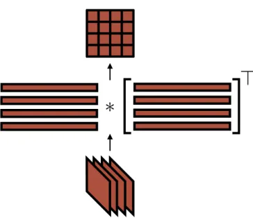
Figure 2.2: Computing the Gram matrix from the activation maps of a layer. Activation maps are first reshaped to row vectors, then the Gram matrix is realized by computing a matrix multiplication between the row-vectorized activation maps and their transpose.

2.2.2 The Gram matrix as a texture metric

Before explaining the Gram matrix as a suitable texture metric, it is necessary to

first understand the mathematics behind it. The Gram matrix, G ₂ Rn⇥n_{, of a}

set of m-dimensional vectors, v1, . . . , vn 2 Rm, is the symmetric matrix of inner

products, whose entries are given byGij =hvi, vji. Essentially, the Gram matrix is

a covariance matrix describing which of its input vectors are correlated with each other. In the case of Gatys et al.’s [21] texture synthesis with a ConvNet, the set of vectors used to compute the Gram matrix are row-vectorized activation maps (Fig. 2.2).

The hierarchical feature representations learned by ConvNets have been shown

to be powerful for diﬃcult visual perceptive tasks such as object recognition

(30)

hand-crafted approaches. Significantly, Movshon and Simoncelli [44] have suggested that given the texture-like features that can be captured in the intermediate stages of these ConvNets, images synthesized from these representations may prove useful as stimuli in perceptual or physiological investigations. This suggests that Con-vNets may be a suitable basis for modelling textures, and consequently, texture synthesis.

In texture synthesis, the Gram matrix computed on activations measures the amount that co-located features tend to activate together. It transforms the spatially-varying feature space into a stationary, spatially-invariant one. Since textures exhibit stationary statistics (i.e., the visual content is spatially homoge-neous), by computing Gram matrices across several layers, a stationary, multi-scale representation of the input image in terms of its texture information is achieved.

2.2.3 Image style transfer

In subsequent work, Gatys et al.’s [22] texture model was used in image style

transfer, where the style of one image was combined with the image content of another to produce a new image. This was achieved by appending an additional term to Eq. 2.5 that enforced the synthesized texture to match the semantic content of the given content image. Specifically,

L= 1 Lstyle X l kGl Gˆlk2 F + 1 Lcontent X l kAl Aˆlk2 F , (2.6)

where Lstyle and Lcontent are the number of VGG-19 layers used when computing

Gram matrices and activation maps, respectively. Gram matrices are computed on the same layers as before, and activation maps are computed on layerconv4_2.

(31)

To briefly review, the Gram matrix of activation maps conveys a notion of texture, or “style”, describing which features tend to activate together. Although the style of the style image is preserved, the global arrangement of its features are not. By including the objective of matching the features of the content image, however, the global arrangement of semantic image content from the content image is preserved. This results in a synthesized image that contains the content of the content image and the style of the style image. The idea of transferring style from one image to another serves as a loose inspiration for the novel dynamics style transfer enabled by the proposed two-stream model. Although with dynamics style transfer, content is not preserved, as it is only a transfer of texture dynamics encompassed by a texture synthesis process.

2.3 Dynamic texture synthesis

Dynamic textures extend from static textures with an additional temporal dimen-sion. The stationarity of spatial statistics of static textures also applies to the temporal domain of dynamic textures.

Unlike static texture synthesis, dynamic texture synthesis has not been as deeply explored. Loosely related—although tangential to dynamic texture

syn-thesis and the proposed dynamics style transfer—Ruder et al. [53] extended the

image style transfer model of Gatys et al. [22] to video by using optical flow to enforce temporal consistency of the resulting imagery. Although their model pro-duced a video output, their core approach focused on an analysis of static style on a per-frame basis. This is tangential to the proposed approach since dynamic textures require an analysis across space and time.

(32)

Variants of linear autoregressive models have been studied [60, 13, 64, 19] that jointly model the appearance and dynamics of spatiotemporal patterns. More re-cent work has considered ConvNets as a basis for modelling dynamic textures. Xie

et al. [67] proposed a spatiotemporal generative model where each dynamic tex-ture is modelled as a random field defined by multiscale, spatiotemporal ConvNet filter responses and dynamic textures are realized by sampling the model. Unlike the proposed approach, which assumes pre-trained fixed networks, Xieet al.’s [67] approach requires their ConvNet weights to be trained using the input texture prior to synthesis. The manner in which they model dynamic textures appears to limit synthesis to a reconstruction, not an extrapolation, of the original sequence, limiting the generalizability of their approach, e.g., synthesizing textures beyond the spatiotemporal extent of the input. A recent unpublished work by Funkeet al. [20] described preliminary results extending the framework of Gatys et al. [21] to model and synthesize dynamic textures by computing a Gram matrix of filter acti-vations over a small spatiotemporal window. In contrast, the proposed two-stream filtering architecture is more expressive as the dynamics stream is specifically tuned to spatiotemporal dynamics. Moreover, the factorization in terms of appearance and dynamics enables a novel form of style transfer, where the dynamics of one pattern are transferred to the appearance of another to generate an entirely new dynamic texture. This work is the first to demonstrate this form of style transfer.

2.4 Representations of dynamics

Numerous representations of dynamics in temporal imagery have been explored, each with their own limitations and level of abstraction. Figure 2.3 illustrates an

(33)

no commitment over commitment

raw signal

optical flow

level of commitment

distributed measurements

of spacetime orientation

Figure 2.3: Dynamics representation spectrum (adapted from Derpanis [11]). Common abstractions of dynamics of temporal imagery and their respective level of commitment to an underlying model.

organization of several extant representations of temporal imagery dynamics. At one extreme, no commitment to an abstraction is made, the raw pixelwise intensity is used directly. This representation fails to leverage the rich underlying structure in the data. The remaining representations are discussed below.

2.4.1 Optical flow

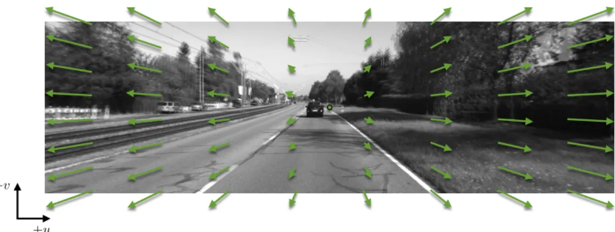
At the other extreme of Fig. 2.3, a two-dimensional (2D) vector field is used to represent the dynamics of the input temporal imagery. This vector field is known as optical flow. It is used to represent the apparent motion of image pixels be-tween two consecutive frames that is caused by the movement of objects or the camera. Each vector in the 2D vector field represents a displacement consisting of a horizontal and vertical component, describing the movement of pixels from one frame to the next. Figure 2.4 provides a visualization of optical flow. The recovery of optical flow from temporal imagery has long been studied in com-puter vision. Traditionally, it has been addressed by handcrafted approachese.g., [33, 43, 52]. Recently, ConvNet approaches have been demonstrated as viable

(34)

+u +v

Figure 2.4: Optical flow visualization. Optical flow is a 2D displacement vector field used to represent the apparent motion of image pixels between two consecu-tive frames, caused by the movement of objects or the camera. Pictured are two, super-imposed, consecutive frames taken from the KITTI dataset [24]. The corre-sponding optical flow is visualized as an array of green arrows. Note that this is just a sample of the motions that optical flow can characterize.

alternatives [14, 34, 51, 68].

A limitation of optical flow is its reliance on a single coherent movement for each pixel and its underlying assumption on brightness constancy, which is diﬃcult to justify for the spectrum of dynamics one encounters in the real world. Examples of dynamics that optical flow fails to capture include flickering, semi-transparent motion, and stochastic dynamics. These are some of the dynamics typically ex-hibited by dynamic textures. Therefore, optical flow is not a suitable substrate for representing the spectrum of dynamics in dynamic textures.

2.4.2 Marginalized spacetime oriented energies

Between the two extremes lies the representation of dynamics that aims to cap-ture a distribution of measurements of spacetime orientations in the input tempo-ral imagery. Unlike flow-based analyses that focus on the apparent motion (i.e.,

(35)

translation) present in the data, measurements of spacetime orientations take a

geometric and generalized approach in capturing spacetime structures: oriented

structures in the spatiotemporal domain that manifest themselves as motion or non-motion,e.g., flickering, stochastic dynamics, etc.

Previous work [3, 17, 30, 56, 65, 48, 12] has shown that the velocity of image content (i.e., motion) can be interpreted as a 3D oriented structure in the x-y-t spatiotemporal domain. Furthermore, in the frequency domain, the signal energy of these oriented structures lie on a plane through the origin where the slant of the plane is defined by the velocity of the image content. For example, in the case where a spacetime structure is defined by the image velocity (u, v)>, the unit normal of

the plane is given by nˆ = (u, v,1)>/||(u, v,1)>||. Hence, energy models of visual

motion, like those presented in these works, are described as “oriented energy” or “motion energy” models, and they attempt to identify this orientation-plane (and hence the pattern’s velocity) via a set of image filtering operations. Specifically, given an input image sequence, these models consist of an alternating sequence of linear and non-linear operations that yield a distributed representation (i.e., implicitly coded) of pixelwise optical flow. These models have been motivated and studied in a variety of contexts, including computer vision, visual neuroscience, and visual psychology

Whereas motion indicates a single, dominant orientation in the spatiotempo-ral and frequency domains, non-motion can indicate an unconstrained, undercon-strained, multi-dominant, heterogeneous, or isotropic orientation. For example, an unconstrained orientation corresponds to structure-less imagery (e.g., image of a clear sky) in the spatiotemporal domain and point energy response in the origin in the frequency domain; and a multi-dominant orientation corresponds to multiple,

(36)

super-imposed spacetime structures in the spatiotemporal domain (e.g., waterfall over a stationary background) and multiple, super-imposed oriented planes in the frequency domain. These, along with the other orientations, are visualized in Fig. 2.5.

This thesis adopts the Marginalized Spacetime Oriented Energy (MSOE) ap-proach of Derpanis and Wildes [12] in representing the observed distribution of

dynamics (i.e. motion and non-motion) of an input dynamic texture. They

con-jectured that the constituent spacetime orientations for a spectrum of common visual patterns (e.g., dynamic textures) can serve as a basis for describing the temporal variation of an image sequence. They successfully applied their model for the task of dynamic texture recognition; here it is used for the task of dynamic texture synthesis. Significantly, a completely analytically-defined oriented energy ConvNet model provides the current state-of-the-art for the related task of dy-namic texture recognition [28]. The proposed two-stream architecture adopts the MSOE model by encoding it as a ConvNet that serves as the representation of observed dynamics of input dynamic textures—the dynamics stream. The same computational steps are used, however, the handcrafted filters of the MSOE model are not used and are learned instead so that they are better tuned to deal with the noise distributions encountered in natural imagery. The construction of the ConvNet is discussed in the next chapter and the MSOE model is reviewed here.

(37)

Figure 2.5: Dynamic texture spectrum (figure from Derpanis and Wildes [12], Copyright c 2012, IEEE). The top and middle rows depict prototypical dynamic textures in the frequency and spatiotemporal domains, respectively. From left-to-right, an increasing amount of spacetime structures are superimposed in a texture. The bottom row depicts a seven bin histogram of the relative spacetime-oriented structure (or lack thereof) present in each dynamic texture. The first histogram bin captures lack of structure. The remaining histogram bins from left-to-right correspond to spacetime orientations selective for static, rightward motion, upward motion, leftward motion, downward motion and flicker structure.

(38)

Given input temporal imagery, I₂RT⇥H⇥W _(time _⇥_height _⇥_{width), a bank}

of oriented 3D filters, e.g., Gaussian third derivative filters G3 2RT⇥H⇥W_{, which}

are sensitive to a range of spatiotemporal orientations, are each applied:

Eˆ_✓ =G3_✓_ˆ_⇤I , (2.7)

where⇤denotes convolution, and G3_✓ˆ is a Gaussian third derivative filter oriented in the direction of the 3D unit vector_✓ˆ_{which lies along the filter’s symmetry axis.}

Each of these filtering operations results in a spacetime volume of filter responses, Eˆ_✓. These filter responses are then rectified (squared) and pooled over local space-time regions to make the responses robust to the phase of the input signal, i.e., robust to the alignment of the filter with the underlying image structure:

¯

Eˆ_✓ = X

(x,y,t)2⌦

Eˆ_✓(x, y, t)2 . (2.8)

At this point, each oriented energy measurement includes measurement of spatial orientation. This means that spatial image structures will aﬀect the responses of the bank of oriented filters, making them dependent on spatial appearance. This dependence is unwanted as it can occur at an otherwise coherent dynamic re-gion,e.g., a surface with varying spatial appearance exhibiting a single, dominant motion. Thus, a description consisting purely of pattern dynamics is sought. To remove this diﬃculty, the spatial orientation component of each filter is discounted via “marginalization”. Specifically, filter responses consistent with the same

(39)

tem-poral orientation (not necessarily the same spatial orientation), _✓ˆ_i_{, are summed:} Eˆn = N X i=1 Eˆ_✓_i , (2.9)

wherenˆ denotes the unit normal of the plane in frequency-space that the spacetime

structures captured by these filters lie upon (implicitly describing a single temporal

orientation), and N denotes the number of these filters. These responses provide

a pixelwise distributed measure of which spacetime structures (discounting spatial information) are present in the input. However, these responses are confounded by local image contrast that makes it diﬃcult to determine whether a high response is indicative of the presence of a spacetime structure or simply due to high image contrast. To address this ambiguity, an L1 normalization is applied across oriented filter responses which results in a representation that is robust to local appearance variations but highly selective to spacetime orientation:

ˆ Eˆni = Eˆni PM j=1Eˆnj +✏ , (2.10) where _Eˆˆ_n

i denotes an oriented filter response from Eq. 2.9 corresponding to a

plane in frequency-space with unit normal nˆi, and✏ is a small value (e.g.,1e 12)

(40)

Chapter 3 Technical approach

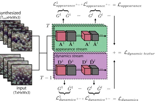
The proposed two-stream approach consists of an appearance stream, representing the static (texture) appearance of each frame, and a dynamics stream, representing temporal variations between frames. Each stream consists of a ConvNet whose activation statistics are used to characterize the dynamic texture. Synthesizing a dynamic texture is formulated as an optimization problem with the objective of matching activation statistics between the target and synthesized textures. The dynamic texture synthesis approach is summarized in Fig. 3.1 and the individual pieces are described in turn in the following sections.

3.1 Texture model: Appearance stream

The appearance stream follows the static texture model introduced by Gatyset al. [21] which was summarized in the previous chapter (Sec. 2.2.1). To briefly review, the key idea is that correlations between activation maps (i.e., normalized Gram matrices) in a ConvNet trained for object recognition (e.g., VGG-19 [58]) capture

(41)

synthesized (ToutxHxWx3) input (TxHxWx3) appearance stream dynamics stream … … … … Ldynamic texture A1 Aˆ1 Al Aˆl + Ldynamics = =

L

appearance

=

T T 1 D1 Dˆ1 Dl Dˆl Llappearance L1appearance Gl Gˆl G1 G

}

ˆ1

}

+…+ +… … … L1dynamics Lldynamics Gl Gˆl G1 Gˆ1 +…₊ ₊…

}

…

}

…

Figure 3.1: Two-stream dynamic texture generation. Two sets of Gram matrices represent a dynamic texture’s appearance and dynamics. Matching these statis-tics allows for the generation of novel textures as well as style transfer between textures. Here, Gl _and _G_ˆl _{are the Gram matrices of activations} _Al _and _A_ˆl _(or _Dl

and _Dˆl_{) corresponding to the target and synthesized sequence, respectively,}

com-puted at layerl of the appearance stream (or dynamics stream) and averaged over

time T (or T 1). _Ll

appearance is the appearance loss at layer l, computed as the

squared Frobenius norm between Gl _and _Gˆl _{from the appearance stream.}

Simi-larly,Ll

dynamicsis the dynamics loss at layerlfor the dynamics stream. By summing each loss computed at various layers, we arrive at Lappearance and Ldynamics, which, when summed, form the combined dynamic texture loss, Ldynamic texture, that is to

be minimized.

texture appearance. The same publicly available normalized VGG-19 ConvNet [58]

used by Gatys et al. [21] is used here. The proposed appearance stream utilizes

this model by simply applying it indepedently to each frame of the synthesized and target texture.

(42)

3.1.1 Target texture appearance

To capture the appearance of an input dynamic texture, an initial forward pass through VGG-19 is performed with each frame of the image sequence to compute the feature activations (filter responses), Alt ₂ _RNl⇥Ml, for various levels in the

network, whereNlandMldenote the number of feature activations and the number

of spatial locations of layer l at time t, respectively. The auto-correlations of the filter responses in a particular layer are averaged over the frames and encapsulated by a Gram matrix, Gl₂_RNl⇥Nl_{, whose entries are given by:}

Gl_ij = 1 T NlMl T X t=1 Ml X k=1 Alt_ikAlt_jk , (3.1)

where T denotes the number of input frames and Alt

ik denotes the activation of

feature i at location k in layer l on the target frame t.

3.1.2 Synthesized texture appearance

The synthesized texture appearance is similarly represented by a Gram matrix,

ˆ

Glt₂_RNl⇥Nl_{, whose activations are given by:}

ˆ Glt ij = 1 NlMl Ml X k=1 ˆ Alt ikAˆltjk , (3.2) where _Aˆlt

ik denotes the activation of feature i at location k in layer l on the

(43)

3.1.3 Appearance loss

The appearance loss, Lappearance, is defined as the temporal average of the mean squared error between the Gram matrix of the input texture and that of the synthesized texture computed at each frame:

Lappearance = 1 LappTout Tout X t=1 X l kGl Gˆlt_k2_F , (3.3)

whereLapp is the number of VGG-19 layers used to compute Gram matrices, Tout

is the number of frames being generated in the output, andk·kF is the Frobenius

norm. Consistent with previous work [21], Gram matrices are computed on the following layers: conv1_1,pool1,pool2,pool3, andpool4. Through systematic eval-uation, Gatyset al. [21] reported these layers were qualitatively superior to other layer subsets for static texture synthesis. Furthermore, they reported that only a subset of layers are required to synthesize textures that are almost indistinguish-able from the input texture, so long as the chosen layers span a wide spectrum of receptive fields (i.e., using early, mid, and later layers of the network).

3.2 Texture model: Dynamics stream

Parallel to the appearance stream ConvNet is a ConvNet designed for captur-ing texture dynamics. There are three primary goals in designcaptur-ing this dynamics stream.

1. The activations of the ConvNet should represent the temporal variation of the input pattern.

(44)

2. The activations should be largely invariant to the appearance (i.e., spatial content) of the images (which should be characterized by the appearance stream described above).

3. The dynamics representation should be diﬀerentiable to enable synthesis via a ConvNet.

By analogy to the appearance stream, an obvious choice is a ConvNet archi-tecture suited for computing optical flow (e.g., [14, 34]) which is naturally diﬀ er-entiable. However, with most such models it is unclear how invariant their layers are to appearance. Instead, a novel network architecture is proposed which is motivated by the spacetime-oriented energy model [12, 56].

3.2.1 Review: Marginalized spacetime oriented energies

This section is only intended to briefly review the aspects of the Marginalized Spacetime Oriented Energies (MSOE) model [12] that are most relevant to the following section; a more thorough overview can be found in the previous chapter (Sec. 2.4.2).

A significant limitation of optical flow is its reliance on a single coherent move-ment for each pixel and its underlying assumption on brightness constancy, which only partially describes the dynamics one may encounter in the real world, and thus in dynamic textures. In response, Derpanis and Wildes [12] showed that the constituent spacetime orientations for a spectrum of common visual patterns can serve as a basis for describing the temporal variation of an image sequence. Their observation motivated a motion oriented-energy approach to representing dynamics, rather than a flow-based approach. By constructing a set of 3D

(45)

ori-ented filters designed to capture spacetime structures beyond just translational motion, they demonstrated a successful application of the approach for dynamic texture recognition [12].

Motion energy models may form an ideal basis for the dynamics stream of the proposed dynamic texture synthesis ConvNet. As such, the MSOE model proposed by Derpanis and Wildes [12] is used to motivate the network architecture.

3.2.2 ConvNet architecture

Using this model as the basis, the following convolutional network is proposed.

The ConvNet input is a pair of temporally consecutive greyscale images, I ₂

RT⇥H⇥W⇥C _(time_⇥_height_⇥_width_⇥_{channels), where}_C_{= 1} _and_T _{= 2}_{. From here}

forth, the channel dimension (C) will be omitted for simplicity. Each input pair is first normalized to have zero-mean and unit variance (i.e., contrast normalization or “instance normalization” [63]), as follows:

IN =

I µ

+⌘ , (3.4)

whereµis the average pixel value of the input pair, is the standard deviation of the input pair, and ⌘ is a small value (1e 12) to prevent dividing by zero. This

step provides a level of invariance to overall brightness and contrast (i.e., global additive and multiplicative signal variations) as well as eases the training process of the ConvNet [40]. The first layer consists of a 3D convolution over the normalized input pair with a bank of 32 3D filters of size2_⇥11_⇥11(time_⇥height_⇥width),

(46)

resulting in an output of spacetime oriented energy measurements:

EF(x) =F ⇤IN(x) , (3.5)

whereEF denotes the response of filterF (of size2⇥11⇥11) after a convolution,

⇤, centered about x _⌘ (t, x, y). In handcrafted approaches (e.g., [12]), a bank of

oriented 3D Gaussian third derivative filters is often used, which require only 10 orientations as a spanning basis. Moreover, these filters typically exceed a temporal

extent of T = 2to capture a wider range of temporal frequencies. Here, however,

an overcomplete bank of 32 learned 3D filters with a temporal extent of T = 2 is

used. This approach is taken for two reasons. First, 3D Gaussian third derivative filters are one of the many types of filters one can use for measuring oriented energy

(e.g., one can use 3D Gaussian fourth derivative, Gabor, lognormal, or

causal-time filters [11]), so it is not required to restrict the network to a smaller filter bank. Specifically, since these filters are being learned, it is within the capacity of the network to learn a wide variety of oriented filters beyond 3D Gaussian third derivative filters. Second, due to GPU memory limitations, the temporal extent of filters are limited to the temporal extent common for optical flow groundtruth imagery, T = 2. Although this restriction limits the range of temporal frequencies

that can be captured in dynamic textures, it is still eﬀective in enabling dynamic texture synthesis with dynamic textures spanning a wide range of dynamics, as shown in the next chapter.

After computing spacetime oriented energy measurements, a squaring

(47)

make the responses robust to local signal phase:

¯

EF(x) = max

i2⌦{EF(i)

2_} _, _(3.6)

where ⌦ is a 5_⇥5 spatial neighbourhood centered about x. A 2D convolution

follows with 64 filters of size 1_⇥1 that combines energy measurements that are

consistent with the same frequency domain plane:

EG(x) = G⇤E¯F(x) , (3.7)

whereEGdenotes the response of filterG(of size1⇥1) after a convolution. Finally,

to remove local contrast dependence, an L1divisive normalization is applied to each spatial location: ¯ EG(x) = EG(x) kEG(x)k1+✏ , (3.8)

wherek·k1 is the L1 norm computed over the filter responses of all filters and ✏is a small value (1e 12) to prevent dividing by zero.

To capture spacetime orientations beyond those capable with the limited re-ceptive fields used in the initial layer, a five-level spatial Gaussian pyramid is com-puted. Each pyramid level is processed independently with the same spacetime-oriented energy model and then bilinearly upsampled to the original resolution and concatenated:

E(x) = ¯EG(x),E¯G(x#⇥2)"⇥2, . . . ,E¯G(x_#⇥2k 1)_"⇥₂k 1,E¯_G(x_#⇥₂k)_"⇥₂k , (3.9)

(48)

encode encode encode

input

(Nx2xHxWx1) contrast norm flow conv (3x3) 64 filters conv (1x1) 2 filters ReLU

decode

aEPE target flow channel concat (x2) (x4) conv (2x11x11) 32 filters rectify max stride 1 pool (5x5) conv (1x1) 64 filters L1 norm

encode

(x½) (x½) decode

Figure 3.2: Dynamics stream ConvNet. The ConvNet is based on a spacetime-oriented energy model [12, 56] and is trained for optical flow regression. Three scales are shown for illustration; in practice five scales are used.

andk+ 1denotes the number of pyramid levels. This final output of the dynamics

encoding stage is named the “concatenation layer”. Training

Prior energy model instantiations (e.g., [3, 12, 56]) used handcrafted filter weights. While a similar approach could be followed here, instead the weights are learned so that they better deal with the noise distributions encountered in natural imagery. To train the network weights, additional decoding layers are added that take the concatenated distributed representation from the concatenation layer and apply a

3⇥3convolution (with 64 filters), ReLU activation, and a1⇥1 convolution (with

2 filters) that yields a two channel output encoding the optical flow directly. The proposed architecture is illustrated in Fig. 3.2.

(49)

L2 norm) is used between the predicted flow and the ground truth flow as the loss. Since no large-scale optical flow dataset exists that captures natural imagery with groundtruth flow, the assembly of a new dataset was necessary. Videos from an unlabeled video dataset are fed through an existing flow estimator to produce optical flow groundtruth for training,cf. [61]. For the unlabeled video dataset, the UCF101 dataset for action recognition [59] is used as it contains a wide variety of complex movements of natural imagery. The synthetic Flying Chairs dataset [14] was also considered as it contained ground truth optical flow; however, training the dynamics stream on this dataset reduced the overall quality of synthesized dynamic textures. This can be explained by the limited motions and appearances exhibited by the rigid objects in Flying Chairs, which is undesirable for estimating motion of dynamic textures. For producing the optical flow groundtruth, the EpicFlow [52] model is used for its state-of-the-art performance (at the time of experimentation) on optical flow regression.

The distribution of movement directions in UCF101 is biased to left-to-right and right-to-left motions, which is undesirable as dynamic textures are not nec-essarily restricted to certain directions of motion. To combat this dataset bias, geometric data augmentations similar to those used by FlowNet [14] are used to equalize the distribution of movement directions in the generated dataset. Addi-tionally, photometric data augmentations similar to those used by FlowNet [14] are used here as well. These augmentations include an image rotation with a rotation

amount uniformly sampled from the range [ 180 ,180 ]; left-right and up-down

flipping with a50%chance; additive gaussian noise with a sigma uniformly sampled

from the range [0,0.04⇤255]; gamma correction with a gamma value uniformly

(50)

value normally sampled from the distribution N(µ = 0, = 0.2 _⇤255); and a

multiplicative brightness change with the multiplicative value uniformly sampled from the range [0.2,1.4]. Each of these augmentations are done in random order.

The aEPE loss is optimized using Adam [37].

Optical flow is chosen as the proxy task (as opposed to dynamic texture recogni-tion [12]) for learning the multiscale distributed representarecogni-tion of dynamics because of the ease of obtaining large amounts of optical flow groundtruth for training. Al-though optical flow is not a suitable representation of the dynamics in dynamic textures, evidence suggests that it is suﬃcient enough to induce the encoding stage to learn the MSOE model within its representational capacity. For example, in-spection of the learned filters in the initial layer of the encoding stage showed evidence of spacetime-oriented filters, consistent with the handcrafted filters used in previous work [12]. This point is illustrated in Fig. 3.3. Furthermore, and shown in the next chapter (Fig. 4.4), there is evidence that the learned representation of dynamics is largely invariant to appearance, another indication that an MSOE model has been learned.

3.2.3 Target texture dynamics

Similar to the appearance stream, filter response correlations in a particular layer of the dynamics stream are averaged over the number of image frame pairs and encapsulated by a Gram matrix, Gl ₂_RNl⇥Nl_{, whose entries are given by:}

Gl_ij = 1 (T 1)NlMl T 1 X t=1 Ml X k=1 D_ikl(t, t+1)Dl_jk(t, t+1) , (3.10)

(51)

(a) Frame 1 (b) Frame 2

Figure 3.3: Learned spatiotemporal filters in the first layer of the dynamics stream. (a) and (b) each depict a temporal slice of the learned filters (2⇥11⇥11),

op-erating on the first and second frame of an input pair, respectively. Inspection of the learned filters reveals structures consistent with the handcrafted temporal derivative filters used in previous work [12] (e.g., row 3, col 1 captures rightward movement and row 8, col 1 captures down-right movement).

(52)

where Dl_ik(t, t+1) denotes the activation of feature i at location k in layer l on the target frames t and t+ 1.

3.2.4 Synthesized texture dynamics

The dynamics of the synthesized texture is represented by a Gram matrix of filter response correlations computed separately for each pair of frames, _Gˆl(t, t+1) ₂ RNl⇥Nl_{, with entries:} ˆ Gl_ij(t, t+1) = 1 NlMl Ml X k=1 ˆ Dl_ik(t, t+1)Dˆ_jkl(t, t+1) , (3.11) where _Dˆl(t, t+1)

ik denotes the activation of feature i at location k in layer l on the

synthesized frames t and t+ 1.

3.2.5 Dynamics loss

The dynamics loss, Ldynamics, is defined as the average of the mean squared error

between the Gram matrices of the input texture and those of the generated texture:

Ldynamics = 1 Ldyn(Tout 1) T_Xout 1 t=1 X l kGl _G_ˆl(t, t+1)_k2 F , (3.12)

whereLdyn is the number of ConvNet layers being used in the dynamics stream to

compute Gram matrices.

The Gram matrix is computed on the output of the concatenation layer, where the multiscale distributed representation of orientations is stored. While it is tempting to use the predicted optical flow output from the network’s decoder stage, this generally yields poor results as shown in the evaluation. Due to the

(53)

complex, temporal variation present in dynamic textures, they contain a variety of local spacetime orientations rather than a single dominant orientation. As a result, the flow estimates will tend to be an average of the underlying orientation measurements and consequently not descriptive. A comparison between the tex-ture synthesis results using the concatenation layer and the predicted flow output is provided in Chapter 4.

3.3 Dynamic texture synthesis

The overall dynamic texture loss consists of the combination of the appearance loss, Eq. (3.3), and the dynamics loss, Eq. (3.12):

Ldynamic texture =↵Lappearance + Ldynamics , (3.13)

where ↵ = 1e9 and = 1e15 are the weighting factors for the appearance and

dynamics content, respectively. Dynamic textures are implicitly defined as the (local) minima of this loss. Textures are generated by optimizing Eq. (3.13) with respect to the synthesized spacetime volume, i.e., the pixels of the video. Vari-ations in the resulting texture are found by initializing the optimization process using IID Gaussian noise. Consistent with previous work [21], L-BFGS [42] is used for optimization. Dynamic texture synthesis results are provided in Chapter 4.

3.3.1 Incremental texture synthesis

Naive application of the outlined approach will consume increasing amounts of memory (in this case, GPU memory) used by the ConvNet as the temporal extent

(54)

(i.e., number of frames) of the dynamic texture grows; this fact makes it imprac-tical to process and generate longer sequences. Instead, long sequences can be incrementally generated by separating the sequence into subsequences and opti-mizing them sequentially. Fig. 3.4 shows a visualization of the incremental texture synthesis process.

This process is realized by initializing the first frame of a subsequence as the last frame from the previous subsequence and keeping it fixed throughout the optimization. The remaining frames of the subsequence are initialized randomly and optimized as above. This approach ensures temporal consistency across syn-thesized subsequences and can be viewed as a form of coordinate descent for the full sequence objective. Specifically, each subsequence can be viewed as a coordi-nate/direction of the full sequence objective that is to be minimized over, while keeping the other coordinates (i.e., other subsequences) fixed. This approach can also be viewed as a form of non-linear autoregression where the output variable (in this case, the current subsequence) non-linearly depends on its previous values (previously synthesized subsequence) and a stochastic term (randomly initialized frames of the current subsequence). The flexibility of this framework allows other texture generation problems to be handled simply by altering the initialization of frames and controlling which frames or frame regions are updated.

3.3.2 Temporally-endless texture synthesis

An interesting extension that was explored were dynamic textures where there is no discernible temporal seam between the last and first frames. Played as a loop, these textures appear to be temporally endless. This is trivially achieved by

Two-Stream Convolutional Networks for Dynamic Texture Synthesis