NASA TECHNICAL NASA TM X MEMORANDUM

N A S A T E C H N I C A L NASA TM X-72646

M E M O R A N D U M

IS*

DESCRIPTION AND EVALUATION OF THE VIKING LANDER CAMERA PERFORMANCE PREDICTION PROGRAM

By Friedrich 0. Buck, Edward J. Taylor, Daniel J. Jobson, and Carroll W. Rowland

January 1975

This informal documentation medium is used to provide accel erated or special release of technical information to selected users. The contents may not meet NASA formal editing and publication standards, may be re-vised, or may be incorporated in another publication.

NATIONAL AERONAUTICS AND SPACE ADMINISTRATION LANGLEY RESEARCH CENTER,. HAMPTON, VIRGINIA 23665

1. Report No. TM X-72646

2. Government Accession No. 3. Recipient's Catalog No.

4. Title and Subtitle

DESCRIPTION AND EVALUATION OF THE VIKING LANDER CAMERA PERFORMANCE PREDICTION PROGRAM

5. Report Date

January 1975

6. Performing Organization Code

T. Author(s)

Friedrich 0. Huck, Edward J. Taylor, Daniel J0 Jobson, and Carroll W. Rowland

8. Performing Organization Report No.

10. Work Unit No. 9. Performing Organization Name and Address

NASA Langley Research Center Hampton, Virginia 23665

11. Contract or Grant No.

'2. Sponson no Agency Name and Address .

National Aeronautics and Space Administration Washington, D.C. 20546

13. Type of Report and Period Covered Technical Memorandum 14. Sponsoring Agency Code

j 15. Supplementary Notes

j 16. Abstract

A computer program is described for predicting the performance of the

i

| Viking lander cameras. The predictions are primarily concerned with two i objectives: (1) the picture quality of a reference test chart (of which i there are three on each lander) to aid in diagnosing camera performance; and i (2) the picture quality of cones with surface properties of a natural

i terrain to aid in predicting favorable illumination and viewing, geometries

I i

j and operational camera commands„ Predictions made with this piogram are I verified by experimental data obtained with a Viking-like laboratory

I

facsimile camera„

1 7. Key Words (Suggested by Author(s) ) (STAR category underlined)

Image quality

Viking lander camera 14

19. Security Ctassif. (of this report)

18. Distribution Statement

Unclassified - Unlimited

DESCRIPTION AND EVALUATION OF THE VIKING LANDER CAMERA

PERFORMANCE PREDICTION PROGRAM

By Friedrich 0. Huck, Edward J. Taylor Daniel J. Jobson, and Carroll W. Rowland

SUMMARY ;

A computer program is described for predicting the performance of the

Viking lander cameras. The predictions are primarily concerned with two

objectives: (1) the picture quality of a reference test chart (of which

there are three on each lander) to aid in diagnosing camera performance; and

(2) the picture quality of cones with surface properties of a natural terrain

to aid in predicting favorable illumination and viewing geometries and

operational camera commands. Predictions made with this program are verified

by experimental data obtained with a Viking-like laboratory facsimile camera.

INTRODUCTION

Two Viking spacecraft scheduled to land on Mars in 1976 will each use

two facsimile cameras to spatially, radiometrically, and spectrally

characterize the surface. The cameras feature a photosensor array with 12

silicon diodes to provide a variety of imaging modes, including six spectral

bands for color and near-infrared imaging with an angular resolution of 0.12°,

and 4 focus steps for monospectral imaging with an improved angular

resolution of 0.04°. The field of view in elevation ranges from 40° above to

60° below the horizon, and in azimuth is selectable in 2.5° steps up to 342.5°.

encoding by use of 6 linear gains and 32 offsets. The camera scanning rates

are synchronized to the lander data transmission rates of 16,000 bits per

second to two orbiters as relay stations and 250 bits per second directly

to Earth.

The versatility of these cameras demands a carefully designed imaging

strategy to optimize their use. The strategy for the first few pictures must

be based on pre-flight predictions of image quality as a function of

anticipated Mars surface properties and illumination and viewing geometry as

well as on camera characteristics. Thereafter, the strategy can be determined

with the help of the initial pictures.

If the quality of the initial pictures received from Mars concurs

generally with pre-flight predictions, then the basic pre-flight imaging

strategy may be essentially continued for the subsequent investigations. If,

however, the quality of the pictures is degraded either because the cameras are

not performing properly or because the actual Mars optical environment departs

significantly from anticipated characteristics, or because both situations

occur, then the pre-flight imaging strategy may be of little further use. A

flexible camera performance prediction computer program can aid first as a

diagnostic tool in isolating the cause of picture degradation, and thereafter

as a predictive tool in revising the imaging strategy. This diagnostic and

predictive function can be accomplished in the following way.: If the pictures

obtained from viewing one of the reference test charts on the lander agrees

with predictions, then the unexpectedly poor pictures of the scene must have

been caused by differences between the actual and the anticipated Mars

environment. However, if the pictures of the reference test chart do not

least in part, by a degradation in camera performance. (But this latter

situation would not preclude a significant difference between the anticipated

and encountered environment). Whatever the inspection of the initial pictures

and the camera engineering data may reveal, the resultant conjectures about

degraded camera performance and unanticipated scene characteristics can be

entered into the computer by altering pertinent camera and scene parameters

until computational results come into agreement with the initial picture data.

Thereafter, the computer program can again be used to predict favorable

illumination and viewing geometry and camera control settings.

Suitable definitions and mathematical formulations of image quality

criteria were derived in reference 1. This paper describes the camera

. performance program that has been developed from these criteria, and presents

comparisons between predictions and experimental results obtained under i

'.controlled laboratory conditions. The experimental measurements were made

with a laboratory facsimile camera that is similar in performance to the

Viking lander cameras.

SYMBOLS

b normalized diameter of approximated circular area of a cone section, pixels

c normalized diameter of cone base, pixels

D diameter, meters

E electronic frequency response

f lens focal length, meters

g phase angle (see figure 6), degrees

I current, amperes

I

I

signal current normalized to 4>(e, ^» g)

=

1> amperes

i integer

J

1

first order Bessel function

k spatial frequency, line pairs per meter

k camera calibration factor

c

k camera optics factor

k conversion factor between time and spatial frequencies

K wi'dth of line pair of reference test chart tribars, meters

L distance from camera lens in object space, meters

L(u, s) lens spatial frequency response

& distance from camera lens in image space, meters

N number of pixels in a cone section

2

N, spectral radiance, watts/meter -micrometer-steradian

/\

N unit vector normal to surface

n number of overlapping line scans

P(v s) spatial frequency response of circular photosensor aperture

3.

P, spectral radiant power, watts/micrometer

A

Q . quantitization level

r reflectance

R

f

preamplifier feedback resistance, ohm

R, photosensor responsivity, amperes/watt

2

S, solar irradiance above Martian atmosphere, watts/meter -micrometer

S/N ratio of average signal to root-mean-square noise

u dimensionless variable for defocus

v dimensionless variable for radius

V voltage, volts

V signal voltage normalized to t))(e, \, g) = 1, volts

Z cone geometry factor

a target slope, degrees or radians

3 instantaneous field of view or angular resolution, degrees or

radians |

6 . azimuth cone angle increment, degrees--©* radians<

£ angle between emitted radiation and normal to surface (see

figure 6), degrees or radians

c; azimuth angle between object slope and incident radiation

(see figure 6), degrees or radians

9 azimuth angle between incident and emitted radiation (see

figure 6), degrees or radians

l angle between incident radiation and normal to surface (see

figure 6), degrees or radians

K number of pixels per line-pair width of tribars

X wavelength, micrometer

A wavelength integral

p, spectral reflectivity of surface (normal albedo)

T, (i ) spectral transmissivity of atmosphere

T, optical throughput

v frequency, Hertz

<j> illumination scattering function

\l> azimuth angle between object slope and emitted radiation

(see figure 6), degrees or radians

Subscripts: a photosensor aperture c camera e electronics i integer £ lens m mirror n noise o flat surface q quantization w window

+ brighter than flat surface

darker than flat surface

The symbol A in front of a parameter indicates a peak or peak-to-peak

variation of that parameter. The bracket < > around a parameter indicates

a criterion which is to be estimated.

IMAGE QUALITY CRITERIA AND PREDICTION PROGRAM

Image quality criteria that have been formulated in refarence 1 are

briefly reviewed, and the computer program that is based on these criteria

is described. It should be pointed out in order to avoid possible confusion

that some details of the formulations obtained from reference 1 have been

changed, and that formulations pertaining to the reference test chart have

Image Quality Criteria

The Viking lander camera has four imaging modes: survey, high-resolution,

color, and near infrared (IR). In the broad-band survey and high-resolution

imaging modes, it is generally desirable to record small spatial details and

slope variations. In the narrow-band color and IR imaging modes, it is

generally desirable to record spectral variations. In addition, it is

generally also desirable in all four imaging modes ,to encompass, but not

exceed, the complete range of radiance variations in the scene with a single

dynamic gain setting. Imagery of the reference test charts on each lander

provides data for checking and calibrating the performance of the camera.

Broad-band imagery. - The capability to resolve small spatial details

and slopes has been defined as the minimum detectable cone diameter and cone

slope with respect to a level surface. A right-circular cone with surface

properties of the surrounding terrain seems intuitively representative of

many features and has no preferred surface orientation azimuthally about its

axis. If the cone angle is chosen to be steep, a condition yielding high

surface contrast, then the detectability of this target becomes primarily a

measure of the camera capability to resolve small detail. I:: the cone angle

is chosen to be shallow, a condition yielding low surface contrast, then the

detectability of the same target becomes primarily a measure of the camera

capability to resolve small slopes.

The cone is probably also the simplest shape for this application. But

it would, nevertheless, be unnecessarily complex to translate rigorously

cone-surface-radiance variations into image grey-scale variations in order

to estimate the detectability of a cone. Instead, the average radiance is

a level surface background, and those regions, including a shadow (if

present), which are darker than the background. The two average reflectance

values and their corresponding areas are then used as approximate target

characteristics in order to formulate an expression for the

average-signal-to-rms-noise ratio of the cone image.

Narrow-band imagery. - The capability to resolve spectral variations

has been defined as the minimum detectable albedo variation. This minimum

detectable variation is taken to be that difference in albedo which results

in an average-signal-to-rms-noise ratio of 3, a level surface being assumed.

Dynamic range. - Knowledge of the statistical distribution (histogram)

of surface radiance would allow the selection of optimum camera dynamic

range setting (that is, gains and offsets as illustrated in Appendix A) for

the complete or a desired part of the radiance range. But the actual radiance

distribution will, of course, not be known until after data have been

received from the lander. It has, therefore, been proposed i:hat a minimum,

mean, and maximum value of the'radiance distribution be estimated, the albedo

and illumination scattering function of the scene being assumed to be uniform

over the landing site. Clearly, the minimum surface radianc2 occurs in

shadows. Since atmospheric scattering on Mars is small (excepting, of

course, during a dust storm) within the spectral range of the camera silicon

photosensors, shadows will exhibit negligible radiance. Hen;e, for the

purpose of selecting a camera offset, minimum radiance may b; defined as zero.

The mean radiance is defined as the radiance of a level surface for a given

viewing geometry. The maximum radiance is defined as the radiance of a

Reference test chart imagery. - The reference test chart (see

Appendix C) provides 11 grey scales to calibrate the radiometric response and

3 sets of tribars to check the frequency response of the camera; in addition,

it provides three color patches to aid the construction of color images.

Camera Performance Prediction Program

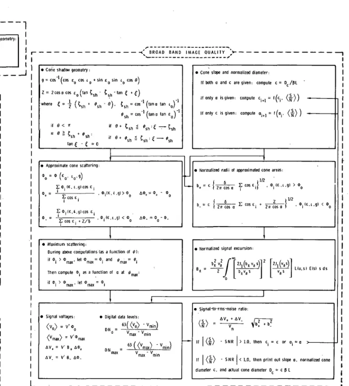
Figure 1 presents a block diagram of the .camera performance prediction

program with all pertinent equations. The program is divided into three

basic parts: input data, interface relations, and camera performance or

image quality computations. The latter, in turn, can be divided into three

sections: image quality of the reference test chart, and narrow-band and

broad-band image quality of the scene.

Input data. - The input data consists of camera characteristics, spatial

and reflectance data of the reference test chart, optical data of the

environment, and illumination and viewing geometry. All of this data must

be readily interchangeable during mission operations. But since the process

of modification is primarily a computer interface function, it: is not

further discussed here. The input data used in this paper to evaluate image

quality computations are given in appendices as follows:

1. Appendix A presents a description of the laboratory J'acsimile

camera that is used in the experiments. The performance characteristics of

this camera are similar to those of the Viking lander cameras

2. Appendix B presents the irradiance characteristics of the National

Bureau of Standard (NBS) lamp and the floodlight used as light sources for

the experiments.

of the Viking reference test chart.

4. Appendix D presents pertinent characteristics of the surface

material used for the broad-band image quality experiments, and the

Meador-Weaver illumination scattering function (ref. 2) that describes the diffuse

reflectance of this material as a function of its physical properties such

as particle size, single-particle albedo, and compactness.

Interface relationships. - The interface relationships primarily

trans-late the input data and camera commands into quantities and units used by

the image quality computations.

The more important computations are:

1. Most wavelength-dependent integrations, including in particular

those integrations that are required to determine the surface radiance and

camera response weighted average wavelength, A, the photosensor signal

current, I', and preamplifier output voltage, V, normalized to <J>(e, l> g) =

2. Normalized camera parameters for the photosensor aperture radius,

v , and defocus, u. a

3. The conversion factor k between the time frequency, V, of

electrical filters and spatial frequency, s, of optical filters.

4. The camera selectable dynamic range, which extends from V . to mm

V , as determined by the offset and gain commands. (The factor 0.216 is a IH3.X

constant negative offset in the video electronics).

5. The total camera rms noise, V , which consists of the photosensor

array electronic noise, V , and the quantization noise, V . The effective

electronic noise bandwidth BW is reduced by the factor n if a line is

6. The overall electronic frequency response, E(v), is the product of

the frequency response of the photosensor preamplifier, E.(v) , the analog

video electronics, E (v), and the running mean integrator used for

analog-to-digital conversion; the integration time is t /2, and t is the time between

s s

samples.

Image quality; reference test chart. - The spectral radiance, W, A,r, of the reference test chart and the spectral power falling on the photosensor

are computed, assuming the illumination scattering function of the target

to be Lambertian and the viewing angle normal. The results lead directly to

the computation of the photosensor signal current, preamplifier output

voltage, and digital data'level. Computations for the tribar peak-to-peak

signal account also for the frequency response of the lens, pinhole, video

electronics, and sampling process. The frequency response computation

includes the first three terms of the square-wave amplitude response as a

function of the camera sine-wave frequency response. The sampling process

generates a signal which is statistical rather than deterministic in nature.

The factor -. accounts for an average reduction in signal contrast; the

actual signal may have a slightly higher or lower contrast.

Image quality: broad-band. - A cone with a normalized base diameter c

(i.e., the actual diameter divided by the pixel diameter) and slope a has

been selected to represent small spatial details or slopes. The program will

compute either one of three alternatives: (1) If both a and c are given,

the program will compute the resultant signal-to-noise ratio. (2) If only

a is given, it will compute the minimum detectable cone diameter, that is,

that value of c which results in a signal-to-noise ratio of SNR; SNR is an

compute the minimum detectable cone slope. Several computational iterations

are required for the last two alternatives.

The first step is to compute the average value of the illumination

scattering function over those regions of the cone which are brighter than a

level surface background (<J>,) , and those regions, including a shadow (if

present) , which are darker than the background (<j>_) . Several lighting and

viewing geometries must be carefully accounted for when computing the cone

geometry factor Z, as explained in detail in reference 1. The second step

is to compute the areas of the brighter and darker than background cone

surface; these areas are then assumed to be circular with a normalized

signal excursion of these two circular areas, B+ and B_, in order to account

for the camera frequency response (including defocus blur).

Together with the previously computed normalized signal voltage V,

these results lead directly to the signal excursion AV and signal-to-noise

ratio S/N. If both a or c are given, then this signal-to-noise ratio is

printed out. If either a or c are given, then a test is performed to

determine if the signal-to-noise ratio is approximately equal to SNR. If

not, then a value of a or c is estimated and all computations are repeated.

Reiterations are performed until the value of a or c results in a

signal-to-noise ratio approximately equal to SNR.

Image quality: narrow-band. - The noise-equivalent radiance and the

minimum detectable albedo difference are directly computed from previously

COMPARISON OF COMPUTER PREDICTIONS AND

EXPERIMENTAL MEASUREMENTS

Two parts of the image quality prediction program need to be confirmed

by experimental measurements; namely, the formulations that are concerned

with the reference test chart and the cone targets. All other formulations

contained in the program are either conventional or very simple, and the

computer program of the formulations has been?checked by independent

computations.

It is of considerable interest to determine the agreement that can be

obtained between predictions and experimental results under carefully

controlled laboratory conditions. This agreement depends, of course, not

only on the accuracy of the formulations but also on the accuracy with which

camera and target characteristics are known. This limitation includes, in

particular, the illumination scattering function of the basalt: material used

for the cone targets (see Appendix D).

Reference Test Chart Images

Predictions are compared to experimental results for four reference

test chart pictures. The facsimile camera was located 1.0 m ilrom the chart

and viewed it normally (e = 0°). A NBS lamp (EPI 1577) was located 60 cm

from the chart and illuminated it at an angle of 20° from normal (i = 20°).

Three of these images are shown in figure 2: the first image was obtained

in the so-called Hi-Res 1 mode, which has an instantaneous field of view of

0.044° and in-focus distance of 1.9 m; the second image was obtained in the

Hi-Res 2 mode, which has the same instantaneous field of view but an in-focus

distance of 2.7 m; and the third image was obtained in the Survey mode, which

has an instantaneous field of view of 0.132° and an in-focus distance of

3.7 m. A fourth image (not shown) was obtained in the color mode, which has

the same instantaneous field of view and in-focus distance as the Survey

mode but uses a red, green, and blue filter during alternating line scans.

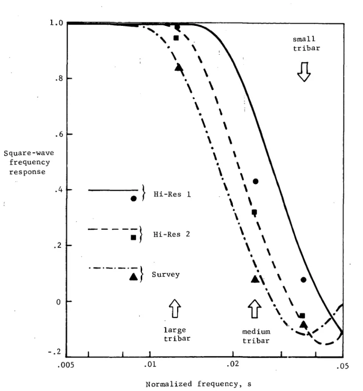
Image details of the three tribars are particularly interesting because

they reveal much about the overall camera performance. The large tribar is

distinctly reproduced in all three imaging modes. Contrast of the medium

tribar is slightly reduced in the Hi-Res 1 mode, significantly reduced in

the Hi-Res 2 mode, and reduced to near the threshold level in the Survey mode.

The smallest tribar is resolved at a very low contrast in the Hi-Res 1 mode,

and gives rise to a so-called false resolution in the other two modes (i.e.,

in this case two rather than three bars).

Table I presents a listing of predicted and measured signal values for

one of the grey patches, the three color patches, and the thr^e tribars. The

good agreement between predictions and measurements for the grey patch

(4 percent on the average) results essentially from the fact that both camera

and reference test chart reflectance calibrations have been made relative to

magnesium carbonate (Mg CO ), using the same NBS lamp. The slightly less

favorable agreement for the color patches (15 percent for red and 7 percent

for green .and blue, on the average) results from the fact that accurate

absolute reflectance measurements have not been made yet for these patches.

It may be concluded that predictions of the radiometric throughput of the

camera are accurate to within 10 percent, which is near the accuracy of the

The agreement between predicted and measured tribar contrast is better

for the largest tribar (9 percent on the average) than for the two smaller

tribars. The reason for the poorer agreement for the smaller tribars is

easiest explained with-the aid of figure 3, which presents the predicted

camera square-wave frequency response and the normalized measurements of the

tribar contrasts. It can be seen that the fundamental tribar frequency

components near the steep slope of the curve and near zero result in the i

largest percentage disagreements. Such disagreements can readily result

from small errors in camera focus adjustments, camera-to-target distance

measurements, and tribar widths. It should be observed in particular that

the combination of highest camera defocus blur and smallest tribar does not

lead to the largest percentage disagreement since the fundamental tribar

frequency component occurs at a shallow inflection rather than steep slope of

the camera frequency response curve. Nevertheless, predictions and

measure-ments agree sufficiently well so that any appreciable image contrast

degradation caused by a camera problem can be effectively simulated.

Cone Images

Figure 4 presents a typical image of a cone, and a computer printout of

the same data which gives the quantization level of each picture element

(pixel). The signal-to-noise ratio of a cone is evaluated from this

experi-mental data as follows: First, the evaluator outlines the part of the cone

that is brighter than the background and the other part that is darker

(including shadow, if present). Second, he records the number of pixels,

N , in each section as well as their quantization levels, Q . The effective

5

'V

and the average signal excursion is

where Q is the background quantization level, and k the conversion

factor from quantization level to signal voltage; Q. > Q for AV , anc*

Q. < Q for AV_. Finally, the average-signal-to-rms-noise ratio is given

by the expression (ref. 1)

S AV+ + AV

V 2 2

N V b* + b n +

-where V is the rms value of the noise, n

The evaluator has to make somewhat subjective judgments during the

first step of the experimental evaluation whether or not he should include

a pixel along the boundary of the cone image as part of the cone. Errors in

judgment can be expected to lead to small errors in the final results for cone

images which contain many pixels (200 or more) as shown in figure 4; however,

the evaluation of such cones is very tedious. Cone images containing few

pixels (20 to 80) were therefore independently evaluated by three persons to

characterize typical variations in experimental results that are introduced by

their different judgments. Results presented in figure 5 show a typical

spread of experimental results. On the basis of these results, it was decided

(2) several cones that contain fewer pixels (about 40) per cone to check on

proper trends of the variations of predicted signal-to-noise ratios with a

variety of cone slopes and illumination and viewing geometry. A defining

diagram of the illumination and viewing geometry is shown in figure 6.

t

Figure 7 presents three large cone images together with predicted and

experimental results. Interesting intermediate results are the number of i

pixels contained in the brighter and darker-than-background parts of the

cone, N ; the final result is signal-to-noise ratio, S/N. Results indicate

that the experimentally determined signal-to-noise ratios tend to be slightly

higher than the predicted values.

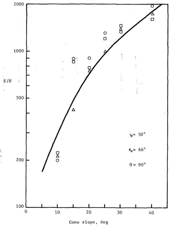
Figure 8 presents signal-to-noise ratio predictions and experimental

results for seven cones with equal base diameters (3 cm) but different slopes

(5° to 40°). The incident (i = 70°) and emission (e = 60°) angles were

kept constant, while the azimuth angle (6) between illumination and viewing

direction was varied in four steps from 45° to 180°. The average distance

from the camera to the cones was 1.4 m; the exact distance of each cone from

the camera was not accounted for in the predictions. As can b^ seen, the

predictions are in consistently good agreement with the experimental results,

at least within the accuracy to which the experimental data can be

quantita-tively reduced.

CONCLUDING REMARKS

A computer program for predicting the performance of the Viking lander

cameras has been described, and predictions from this program have been

compared with experimental results. The predictions were concerned with

pictures of a reference test chart and of cones covered with natural (basalt)

material. Predictions of the picture quality of selected reference test

chart features can aid in diagnosing camera performance. Predictions of the

picture quality of cones with surface properties of natural terrains can aid

in determining favorable lighting and viewing geometry and operational camera

commands.

Predictions of the picture quality of selected reference test chart

features were compared with experimental results for several camera imaging

modes, providing different angular resolutions, defocus blur, and spectral

responses. The predictions and measurements for the radiometric throughput

of the camera generally agreed within 10 percent, which is near the expected

accuracy of the absolute radiometric calibration of the Viking lander cameras.

Predictions and measurements of the camera response to three sets of tribars

on the reference test chart agreed sufficiently close so that any appreciable

image contrast degradation caused by a camera problem can be simulated by the

computer program.

Predictions of the picture quality of cones were compared with

experi-mental results for a wide variety of cone slopes and illumination and viewing

geometries. The comparison provided consistently good agreement within the

accuracy to which experimental data could be quantitatively reduced. The

experimentally obtained signal-to-noise ratios of cone pictures depended

somewhat on subjective judgments and tended to be slightly higher than the

predicted signal-to-noise ratios. However, the variations of predicted and

experimental signal-to-noise ratios agreed closely for all variations in cone

slope and illumination and viewing geometry.

that was used to describe the reflection characteristics of the material

used to cover the cones. The illumination scattering function that will

actually be encountered at the landing sites on Mars is, of course, less

certain. This uncertainty suggests that the dependence of picture quality

on lighting and viewing geometry should be investigated for a wide range of

.reasonable illumination scattering characteristics to establish a sound basis

for determining the preprogramed lander commands that automatically direct

camera operations during the first few days on Mars. The Meador-Weaver

illumination scattering function lends itself readily to this task since it

describes the diffuse reflectance of natural materials as a function of their

APPENDIX A

PERFORMANCE CHARACTERISTICS OF THE

LABORATORY FACSIMILE CAMERA

Although the laboratory facsimile camera differs greatly from the

Viking facsimile camera in many design details, it can closely simulate

those performance characteristics of the Viking camera which are important

to this investigation. This appendix presents a general description of the

laboratory camera design, and a detailed description of its performance

characteristics when adjusted to simulate the Viking camera performance.

General Description

A basic block diagram of the laboratory facsimile camera is shown in

figure 9. Radiation from the scene is reflected by the scanning mirror,

captured by the objective lens which has an adjustable aperture, and projected

onto a plane which contains the photosensor aperture. The photosensor - in

this case a silicon photodiode - converts the radiation falling on the

aperture into an electrical current. As the mirror rotates, the imaged scene

moves past the aperture permitting the aperture to scan vertical strips. The

camera rotates in small steps between vertical line scans until the entire

scene of interest is scanned.

The instantaneous field of view is determined by the photosensor aperture

size and distance from the lens. Different instantaneous fields of view can

be obtained by inserting different modules which consist of a photosensor

The mirror line-scan motion is directly controlled by a servo, which,

in turn, is synchronized to a clock pulse rate. An important part of the

servo-control is an accurate mirror position sensor (optical encoder) which

has three functions: (1) it aids the servo-control to achieve a linear

mirror scan synchronously with the clock rate, (2) it allows the selection

of any vertical field of view of the scan (i.e., of an image frame), and

(3) it provides pulses for sampling the video signal. Use of these

servo-derived pulses (rather than the clock pulse) for sampling the video signal

allows the photogrammetric accuracy along the line scan direction to be a

function only of the accuracy of the mirror position sensor, and to be

independent of small deviations from a constant mirror-scanning velocity.

Immediately after each vertical line scan of the scene, a pulse is sent

from the mirror position sensor to the azimuth rotation and filter wheel

logic controls. In the broad-band imaging modes, the filter wheel is

commanded to position an unfiltered opening over the photosensor aperture,

and the azimuth drive (which consists of a steppermotor and harmonic gear) is

commanded to advance at the end of each line-scan by a selectable interval

(in 0.011 degree steps). In the narrow-band imaging mode, the filter wheel

is commanded to rotate a different filter (out of three) over the photosensor

aperture after every line scan, and the azimuth drive is commanded to advance

after every third line scan.

As shown in figure 10, the photosensor signal current is amplified

using a different gain (RfG = R R_/R..) for each channel: high-resolution,

survey, blue, green, and red. The dark signal voltage (i.e., the voltage

level when the mirror is facing the blackened inside of the camera), is

Additional voltage levels can be subtracted from the signal by a programable

digital-to-analog converter. The resultant signal is then further amplified

by a programable gain amplifier and bandwidth-limited by a low-pass filter.

The programable offsets and gains permit the camera to function with selectable

dynamic ranges as illustrated in figure 11. The filter provides adjustable

bandlimiting of noise and signal prior to digital sampling.

Performance Characteristics

The performance characteristics of the laboratory camera, which are

important to this investigation, are the transfer functions of optics and

video electronics and the mirror scanning rate. Most of these

characteristics are listed in Table A-I. In addition, figure 12 presents the

relative responsivity of the photosensor, figure 13 the transmittance of

the color filters, figure 14 the frequency response of the photosensor

preamplifier, and figure 15 the frequency response of the adjustable filter

used to bandwidth-limit the video signal.

The linearity of the video amplification and processing circuits falls

within +1.0 percent of an ideal straight line for all gain settings over the

operating range extending from 0 to 5 V. The accuracy of the offsets is

within +5 mV of the stated value. Exact values for gain and offset are listed

in figure 11. The sample and hold circuit used for drift control has a holding

TABLE A-I

LABORATORY FACSIMILE CAMERA CHARACTERISTICS

Characteristics

Instantaneous field of view, 3, deg

Mirror reflectance, r m

Lens aperture diameter, D, cm

Lens focal length, f, cm

Lens transmittance, T.

Photosensor aperture diameter, D , cm 3.

Photosensor peak responsivity, R , A/W

Photosensor-preamplifier feedback resistor, R,., ohm

Signal equalization amplifier gain, GI

Picture elements per line

Field of view per frame elevation, deg

azimuth, deg; min; max

•

Elevation scan rate, X > deg/sec s

Azimuth stepping rate, deg/sec

Low- Resolution 0.132 0.84 i

1.0

5.5

0.9

0.0124 0.34 0.92 x 109 Survey: 1.56 Red: 15 Green: 36 Blue: 193

512

67.584 0.132; 360

520

Survey: 0.132 Color: 0.044 High- Resolution 0.044 0.84

1.0

5.5

0.9

0.0043 0.27 0.88 x 109 ' 17.5

512

22.528 0.044; 360

520

0.044

APPENDIX B

IKRADIANCE CHARACTERISTICS OF LIGHT SOURCE

Two types of light sources were used in this investigation: National

Bureau of Standard (NBS) lamps and a spotlight. The former were used for

all absolute radiometric measurements, and the latter for most image

quality studies.

NBS Lamp

The NBS light sources are commercial G.E. type DXW-lOOO-watt lamps

that have a tungsten coiled-coil filament enclosed in a 0.95 cm diameter

and 7.6 cm long fused silica envelope, which also contains a small amount of

iodine. The lamps' color temperature range from 3000°K to 3050°K for a dc

current of 7.9 A. Each lamp is supplied by the National Bureau of Standards

with calibration data. Figure 16 presents typical spectral irradiance data

at a distance of 50 cm; the inverse-square law may be used to calculate the

spectral irradiance at distances beyond 50 cm.

Spotlight

The spot light is a 10 KW tungsten lamp with a 61 cm diameter Fresnel

lens. It is supplied with rectified 3 phase, 120 V power, and has an

effective color temperature of approximately 3200°K at the rated power.

However, the following procedure was used to adjust the spotlight to a

better known spectral irradiance: A grey reflectance card was first

illuminated by a NBS light source and scanned by the laboratory facsimile

were equal. The same grey reflectance card was then illuminated by the

spotlight and scanned again by the facsimile camera as before, and the

spotlight current was adjusted until the three color channel outputs were

the same.

The spotlight optics can be adjusted continuously from spot to flood

position. In the full-spot,position, the irradiance is concentrated toward

the optical centerline and drops off rapidly with distance from the center i

line. In the full-flood position, the irradiance is spread over a circular

area of about 76 cm diameter with +5 percent variations in magnitude. For

a setting of 5.5 (near the full-flood position) the irradiance at a distance

of 148 cm (as used during most tests) is 1.67 times the irradiance of the

NBS lamp EPI 1556 at a distance of 50 cm.

APPENDIX C

REFERENCE TEST CHART CHARACTERISTICS

A picture of the reference test chart (RTC) is shown in figure 17. The

paint surfaces concist of 11 grey reflectance patches, three color patches,

and three sets of tribar patterns.

Properties of the RTC which are of concern to this investigation are

normal reflectance (reflectance at zero illumination and emission angle),

illumination scattering function, and tribar dimensions. The normal

reflectances of the grey patches are given in Table C-I. Curves of the

normal spectral reflectance of the color patches are shown in figure 18.

The illumination scattering function for all patches is assumed to be

l Lambertian (i.e., cosine dependence on illumination angle and no dependence

on emission angle). The widths of the individual bars in the tribar

patterns are given in Table C-I.

All data presented here for the RTC are preliminary. Evidence exists

that significant deviations occur from these nominal values for reflectance,

illumination scattering function, and bar widths. These deviations may

account for some of the differences between predictions and measurements that

have been encountered. Measurements of RTC characteristics have also revealed

target-to-target variations. The specific RTC used for measurements must

TABLE C-I

REFERENCE TEST CHART CHARACTERISTICS

Grey Patch Reflectances

Patch Number

1

2

3

4

5

6

7

8

9

10

11

Reflectance

.11

.15

.20

.25

.30

.35

.40

.45

.50

.60

.79

_-. — Tribar Large Medium Small Tribar Widths j Width, mm/£p ', | 6.4

3.3

2.2

27

APPENDIX D

THE ILLUMINATION SCATTERING FUNCTION OF A

PARTICULATE SURFACE OF COLORADO BASALT

Meador and Weaver (ref. 2) have proposed an illumination scattering

function that describes the diffuse reflectance of particulate surfaces as

a function of their physical properties (particle albedo, size, and packing

density). This appendix presents this function, the geometrical relationships

necessary to use it in the prediction program, and the pertinent scattering

and physical properties of the Colorado basalt surface used ia experimental

image quality studies.

The Meador-Weaver Illumination Scattering Function

The scattering function given by Meador and Weaver is (ref. 3)

- £' 8) = cos

+ a., (cos i + cos e))

where i is the angle of incidence, e the angle of emission, g the phase

angle, and a , a , a are empirical parameters that contain information

about the surface. The factor f(l, e, g; a~) is given by

f(l, e, g; a2) = e

1/2

+ v/1 exp{y - -£— (3TT(2£-l)x + 6 x sin~x + 2(2+x2) (1-x2) ) }dx o

all other values should be replaced by f(i, e, g; a~) = 1. The parameters

y, V, and £ are given by

4a (1 + cos g)

v =

3 sin g

?

(cosi + cos e)[cos y 4- cos (g-y)]cos K

sin g cos i cos e

_ _ (cos i + cos e) cos y cos (g-y)cos K

[cos y + cos (g-y)] cos i cos e

The parameter K is the angle between the surface normal and the scattering

plane (the plane containing the incident and emission directions), and y

is the angle between the incident direction and the projection of the surface

normal on the scattering plane. The function 4>(l, e, g) is normalized to

unity at i = e = 0°.

The parameters a , a , and a are empirical parameters which relate

certain physical properties of a surface to its scattering properties. While

precise quantitative relationships between a and the physical properties of

the surface have not yet been established, approximate relationships have

been determined; a and a, are related to particle albedo and size

distributions of the surface, and a» is related to the packing density of

the uppermost particles comprising the surface. A more detailed description

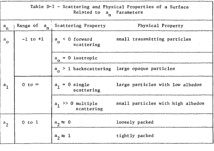
of these relationships as summarized from ref. 3 is given by Table D-I below.

Table D-I - Scattering and Physical Properties of a Surface Related to a Parameters

n

a Range of a : Scattering Property n i n a -1 to +1 o a 0 to °° a2 0 to 1 a < 0 forward scattering Physical Property

small transmitting particles

a =0 isotropic a > 1 backscattering a = 0 single scattering a, » 0 multiple scattering a Ki 0

large opaque particles

large particles with low albedos

small particles with high albedos

loosely packed

a « 1 tightly packed

Geometrical Relationships

The two angular variables K and y in the Meador-Weaver function and

the angles i, e, g, and 6 used in the prediction program are related as

follows:

sin K=sin i sin £ sin sin g

sin y = sin \ (cos e sini - cos 6 cos i sin e) cos K sin g

Properties of the Material Used for Experiments

A surface of Colorado basalt (mafic latite porphry) with a particle

size range of 150 to 300 micrometers and a mean particle size of 180

(D-2)

scattering function of this surface has been measured by Meador and Weaver

(ref. 3) for coplanar values of incident and emission directions. Values

of a were determined iteratively using equation (D-l) to fit their

experimental data. The values of a were determined to be n

a = -0.4 : o

a^ = 0.28 a_ = 0.32

The validity of using the Meador-Weaver scattering function for

non-coplanar geometries of incident and emission directions has not yet been

proven for the Colorado basalt surface.

The albedo of the Colorado basalt surface was measured relative to

that of Magnesium Carbonate (MgCO ) with a light source having a color

temperature of 3000°K and an unfiltered silicon photosensor. The albedo

of MgCO is approximately constant over the silicon photosensor responsivity

range, so that for this particular condition the albedo of bt.salt may be

taken as

/S(A)p a)T (A)R(A)d

-0.97)<0.20)-0.»

where the factor 0.20 is the measured ratio.

REFERENCES

1. Huck, F. 0.; Jobson, D. J.; Taylor, E.J.; and Wall, S. D.: Formulation of Image Quality Prediction Criteria for the Viking Lander Camera. NASA TM X-2802, September 1973.

2. Header, W. E.; and Weaver, W. R.: A Photometric Function for Diffuse Reflection by Particulate Materials. Prospective NASA TN.

3. Weaver, W. R.; Meador, W. E. ; and Wood, G. P.: Values of the Photometric Parameters of Mars and Their Interpretation. NASA TM X-71949, May 1974.

rl CU W $.** w B~S 3S rH PH W 6-«

c

0)

2

s

o Pi W 6^2 T) £ « CO •H PL, CU rt W X B~S U CO >. M CU

1 £

s crt -1 , U W PH W 6-S CM CO CU f* S ••H .... , , . ffi CM w B3 r— 1 CO cu

pi a

•rl PC Pk Referenc e t Char t s <• vO CN rH m H <!• • m r^ m vO ^3-r~ CTi * -3-CM m oo -* co r~ vi-vo M3 CN • m oo m m ro o\ CM • m <)• -j-• m CN m CN m -* CO • m Gre y patch : % reflectanc e m r~- oo r-l rH VD CO CN rH cy> o en r* <y> CN • • • rH in -* r^ oo VO CTN CT> • • • m rH ro m CN •* r*. m o in <r • * • rH CN rH rH O OO <r m ro oo • * CN rH r*. in vo CN f) P^ OO oo r^ o VO rH CO m oo tH CO CO CT» r-« rH CN vO -J- O rH rH m vo vo CTl O- O vo m oo OO rH CO rH r^ O\ * • • oo in oo CN rH VO rH r-~ <N oo O m rH • • • t-~ in oo CT> r-» CN cr> in r-. r~» m oo CO rH VO rH c^ CN m oo m o vo m oo >* vo m oo <r m r^ m oo Colo r patches : Re d Gree n Blu e CT> <Ti cs) CO -tf -* m vo CN <f rH OO O\ CN <O 00 • • * <r i m cy> vo o -* m • • • -* 1 t-~ vo sr rH m CO CO vo P~ rH CN CO • • * CO 1 CO vo CN r-» •* m * • • CO 1 vo o m rH 1^ rH vo •* r-~ O CN m • • • CO 1 00 «* CTi m <• <r • • • CO 1 r-~ co o co <r cr> oo oo oo to co • • • CO 1 00 CO f~~ rH m m -a- i 00 CTi (* <r VO r^ rH CO •* CO • • • <T rH | rH in rH r~ ro m • • • -* rH 1 co c^ co CO VO cy\ o m m o co • * • •<r CN •<r r- rH i*> a\ r*~ •3- CN Oi O-. P-< 0? 0? Oj CO vo vO -J" ,Q . •H CN vO -J-}-l i-l H n) CO M 0) cu co tfl PM o Vl V4 w o>

a

0) o cu PM o •H O •iH Vi PM O O Pu

Si-ll

w

4J p! CU II

s

< I N P U T DATA V

V j

I —^ I N T E R F A C E R E L A T I O N S ,>— 1

Spectrally-dependent camera and environmental parameters: Camera optical throughput: TX c = TX w, TX w2 Tx_m TX

Al = /SXTx ( ' o )( )XTX . cRXd X A2=/X SXTx ( ' o )X| ) TTX . cRXd X

Surface radiance and camera response weighted average wavelength :

• Optical geometry-dependent camera parameters: Laf _ "a _ JL 2 i 'a = L7T " = -Ta kp = 16 D » • Normalized photosensor signal current: I = and preamplifier output voltage: v' =

• Normalized camera parameters:

Photosensor aperture radius: Va = y= (-pj 0

Defocus: U = ^ r IT-) / - / , . / = L f / ( L - l > XSD Mirror scan rate to frequency:v = kv$. ky =

Camera selectable dynamic range: '(lz)

-O.n. 5 Olfset number G.n. s Gain number

• Electronic parameters:

Electronic noise: Total noise:

,1/2

V ( n ) = l' R

Quantization noise: frequency response: sin7rtsu/2 lit, u/2 • Camera: TX . w rTX , w 2 ' rX . m 'TX . / "Da' V RrG-El( w l- E2<u'. . RX. D. f BW. kc

• Environment: • Reference test chart: TX . b -rX . g -rX . r -rr VK1 'K2 'K3

i =1.2. ....11 ^ »

• Illumination and viewing geometry:

i—

I -«^ B R O A D B A N D I M A G E Q U A L I T Y S 1

R E F E R E N C E T E S T C H A R T . I M A G E Q U A L I T Y

L

• Reflectance of color and gray scales:

r ' = r c o s t . r = ^ b. rx g. rx r . fj , where i = 1. 2. . . . 11 • Reflectance excursion of tribars:

r' = fir cost

• Spectral radiance: NX . r = 7SX ' x ( ' o )r'

• Spectral power falling on photosensor aperture: PX . r = *KpNX . r

• Photosensor signal current: [ • Preamplifier signal voltage: V • Digital data level: D

= lc/PX . rTX . cRXd X r =G Rf ' r

"(Vr"Vmin) r vmax vmm

• Number of pixels per line pair width of tribars : K = -^p- K . where K is width of line pair • Normalized frequency of tribars in image plane:

s- T » i i_

s- * TT K /a

• Normalized signal excursion:

is- 4 [A ar1 MM c(i..lsln»A

71

h^t '

iVaS

"

/K

Lj-a-i -*

1

• Photosensor signal current: AIr = kc bSff T R dx • Preamplifier signal voltage: AVr = G R(a lr

_„ .„.. "(V^min) max min N A R R O W B A N D I M A G E Q U A L I T Y • Noise-equivalent radiance: V < N E R > = -T /Nx dX

•' Minimum detectable albedo difference: 3V.

L.

• Cone shadow geometry:

g = cos (cos EO cos i + sin E sin i cos e) Z = 2 cos a cos E (tan t h " C h ' tan f t ( \

where C = 7 ( tsh + *sh ' 8) . 5sh = cos"1 (tana tan t()) ' sh \ o/

II 9 i ^ t 0 :

tan J - £ = 0

• Approximate cone scattering: It = 0 1 £ i Q 1 o V o o / E 0. (E, t.gicos e j *+ E C O S E , - i - -9 - „ - + + o £ OjlE.i.gicos E. £ cos E! +Z/6 ' ' ' ' '9 ° o • Maximum scattering:

During above computations las a function of if}-. i f* i > 0m a x 'l e t C )m a x= ( tia n d *max= *i Then compute <s>.f as a function of a at *max:

t '

• Signal voltages: • Digital data levels: ^V.^ = V' 0 "( vo/ " vminj /„ N -V. ° o D'J° V m a"'V™" \vmax/ ~ v max

,,. „ « 63 ( /V N - V } AVt = V B+A O )t ON _ V \ max/ min/

AV. = V B. 40. maX ma)C min

1

J

• Cone slope and normalized diameter:

If both a and c are given: compute c = D /pi

• Normalized radii of approximated cone areas:

"+ - c I 2;r cos a f C O S Ci( • « j ":- ' - 9| > »o

1 6 Z I172

"- - c 1 2ff cos a r cos Ei " 2^ cos o ) • *i ( E'1 -gl ( *o

• Normalized signal excursion:

Bt ' 2 / b v s " S Llu.sl Els) s d s o L J

1 • SignaHo-rms-noise ratio:

(N) vn ^T^T

If {-jg-} • SNR < 1.0. then print out slope a. normalized cone diameter c, and actual cone diameter D = c p L

M

a

• to (0 3 (-1 O O C U 6 C co co O 4J -C S cu co i^ JJ 4J -4-1 CO CN C M C M-l CO c cfl <N CO *T3 T3 O 01 01 4J C CO CO -i-l 0) O CO U O 4-1 C i-l .C CO O 4-> 4-1 CO M 0) -i-l CO M *O CJ S co 3 4J CO O CO 01 O 0) U-t *-> C <U CJ -H O -i-l C Q.T3 o> C )-i CN CO •O O) 01 U •H cfl CO 4J 4-1 CO fO -H 0 T3 CO CO co 3

* 8

01 m 3 C 4J -H O 0. co a) oi -d1 I O •r4 • CN O 13 <4-l d o en co cy 3 fc i-l O) 3 -H 4J CO > U U •H OfJ "4-1 O. I O •H 0) SC T) (U .-I I-l (U 0) H H *W I CN OI

5

•H 4J O >> o) r-l -i-l O) > -r-l >4-l 4-1 O O <u -o D4 ^1 co Ol 01 •>-<

1.0

.8

.6

Square-wave frequency response

.4

.2

.2 .005 large tribar

.01

.02

_.05

Normalized frequency, s

Figure 3.- Predicted square-wave frequency response of the camera for a target located 1.0m away, and normalized tribar contrast measurements.

in ^ OJ O-J un ID OJ CM — OJ CM OJ r-w ID OJ CM ro CM OJ CM CM G) CM OM un in CM OJ is- tf CM CM ro — • OJ OM in oj OJ CM -rt- ^ OJ CM Ki ^-T OM OJ

<rir

OJ OJ «-" IT, OJ OJ ^j r°o OJ OJ OJ ^T OJ OJ OJ — i p, 1 {-, 1 ISJ I SI in t OJ OJ oj ro OJ OJ OJ OJ cn G) •-1 OJ

^r

—

CM CM KJ ro OJ CM ro -sT OJ OM ro CM f\\ (-, \ I.SJ I -J m G> CM OM — CM OJ CM — * G) OJ OM G) — ' OM CM LD ^ CM OM : %W:

fe- 9

r •

lflllaii»,«i : CM OJ T^-OJ Tf O-j -J OJ TTJ-0-J CM OJ OJ O-J O-J OJ OJ CM TJ CM •sj CM ^ OJ ro OJ un OJ ro OJ G! OJ Ki OJ Ki OJ ro OJ OJ ro CM _ CM OJ OJ , — ( OJ ro f, i l \1 O-J OJ _ OM rf CM ro CM ro OM ro OJ in OJ CM CM U) CM

in

CM

^j-OJ ro OJ in O-J — , OM in O-J TJ-O-J KI OJ

sr

'. ''J rs. OJ KI

—

OJ Tf 1. 'J in OJ OJ 0\J ro OM CM CM CM <N

in

OJ GJ CM .-. i ISI ro CM un OM „ CM O-J OJ ^j-CM ro CM in CM ro CM •sT OJ •st OJ ^lj OJ in OJ OJ OJ ~H OM in OM in OJ OM OJ •3 CM OJ OJ in OJ OJ OJ LD OJ OJ U""J OM rn CM ro CM ( •st 1 OM Ki 1 O-j I r- 1 I XI OJ CM r- i CM ( — ' O-J ( _ OJ ( in c OJ ( [M fM M D ^1 ro [M n M n M n "M T-, M M M "O -••1 •O 'M D M >O "\|

jr

~"J -'•J ~sl D '•-J M "sl

•o

'J — i "sl M M •O M M M O M n M -i 1 SI 0 M 0 M -SI — H M M M un OJ |S-OJ (X_ OJ ro 0-1 un CM ID CM ro OJ OJ O-J OJ CM ro O-j ro CM on CM ro ™ OJ CM OJ 1. '--J ^t OJ OJ Kl Oj O-J CM CM ^j CM ro CM in CM 7^ ro OJ ro O-J ro OJ ro OM OJ CM on CM UJ OJ '-D OJ un OJ |S_ OJ ro OJ in CM in OJ h-OJ in CM TJ OM U3 CM in OJ ^3" ro OJ TJ i. '--J O-J OJ CM ™ OJ TT" CM ro CM O-J OJ Osl CM tj-V OM OM O-J CM in OJ ro OJ 'D OJ rt OJ CO OM |S_ O-J f^ OJ cn CM G) ro in OJ un OJ CO O-i 0 ro is_ OJ r-CM rs. CM CO '. M |S_ OJ r--OJ ro OJ ro OJ *•]'' OJ x-']" OJ OJ CM *— 4 CM ,_ O-J OJ OJ ro i-H OJ •3-CM m ^H CM CM ._ CM _ CM CM CM

ro

O-J IS) •••-J OM ~M -CM OJ OM ••i o.i '• v —.

cn LH TI oj in oj is) is. CD ^r ro on 'Xi ID ^ in — • oj to u. ro CM ro ro *t %r t io ro ro ro ro oj IM OM oj CM o-j r . ;•-; r; oj Q in Q ro — CM co ^r ro ro OM co ID un is. T ^r ro oj CD OM ro ro ^ ~3 *i *\r ro ro ro ro ro o-j CM o-j CM OM CM o-i CM OM o-j OM ift ~* in — • on o~'i cn in in *-? K' o~' ^ ^ ^~ ^ ^-j" ro ^-l* JT ro ro ^ \r •sT ro ro ro KJ ro ro ro CM oj CM OM CM o j oj OM oj ro r- *t ^ — r-- in on r- OM co cn ^ oj t *T *r ro ro OM — • ro KI ^ \r ^r ro ro ro ro ro ro CM CM oj CM OJ CM CM CM OM oj — • ^ OM 'sT cn on ^r ro in ro — • cn cn in in \T — • r<- ro CM ^J ro KI -st 'st ro ro ro ro ro ro ro CM oj oj OM OM CM o-, CM o-j oj co rs. — oj cn un CM •sT oj OM co co un is- iri ^ ro ro CM f r- 1 ro ro •sT %T ro r> j r-n ro ro ro OM CM OM CM o-j oj oj o-j OM o-j OM cn cn — < — ' co in ^r cn un J-D un u"i r- un 'sT ^ — • m CM in ^ CM ro 'sT ^T ro ro ro CM CM CM oj oj oj oj oj OM oj — CM OJ oj in b) ^t GJ in CM OM KI in r-- cn un ro ro T — • CM ID T CM co ro •sT ^r •sT ro M ro ro OM CM oj CM oj oj oj oj o.j CM oj CM OM co — « co is- ro ~-i cn is. -q- T in •sT UT in r^ in —• CM oj — « -« M ^T r- i ro r«n ro OM OM TM OM OM OM OM CM OM OM CM CM CM OM OM M un in OM cn ID co m OM •st — « G) r-- G> OM G) on CM oj E — • ro ro i-o ro CM OM OM OM CM OM CM CM ~- OM oj oj — • cv OM OM oj ro OM — • is. un 'J KI un ro — < so ro ^ T oj GD CM <^< ^^ — * rM ro ro ro CM CM CM CM OM oj oj CM CM OM OM CM CM o-j oj o..1 o-j CM

CM (S3 IS, Un OM O ^ OM CS3 — ' (Ti CTl — • OJ El — • D H . — ' — ' — • ro ro CM CM OM CM CM CM CM o-j — • — CM CM CM OM CM 01 OM r-j CM cn ^t ^^ un r-- '^ KI GI co di co r- r-- co Q CM LO '1 '-• G:> G) co co un UT is. un co on un in un in ID on KI r-- 0 ro CM — < G) ^T in oj CM ^t Lii ^J u~) in ro oj ro in cn co GJ *^ " " ^ CD oj l.£l l£l f-_ CQ — * — i ^ Tj y-i f.j ,-,j p.j Q-, (^ _^ jTT, ^3 L:;. fl.j pj p.j oj oj ui LD cn co oj — CD ro oj ro LD co Q o ro if in ro ^ r-- cn ^f ^ UT N. LO co r-- co GJ EJ 'T r-- r-- cn on o; f"1;; 'st oj G) cn in •sT ro "st un r-- un cn OM in r-- r- r-- co — ro o-i ro 10 CTi ^^ ^ ro CM ro "sT ^ un cn cn cn ro r-- cn CD OM r^ u~' ro cn ~-" — ' — i —i — ' OM O-J O-i O-J IM '-' on co ^ ro — • ro ro ^ q- in ID co un ID on o GJ K — in OM — ' — — ' ~ — — OM OJ O,' O-J OJ OM cn ro uj CM CM CM o-j o-j CM CM ^-T on CM 1 T-J" r- co K s — — • — i — i r-i — i — i — i r-j c ; ,M CM CM GJ \r u~i ro OM — ' oj OM OM ro in m —i \r cn T — er cr. o-; GJ

OJ — • — —i —i — i O.J O-J «- -1 OJ OJ

ID oj 'xT ro OM oj OM OM — • — • \r CD — T un on — < ~:: in in a — i — < — i -< —. — • —i O-J O 0-1 CM OJ

*-> r- on ro OM ro CM OM CM CM un ro r- un T co — ' r' oj — — •

G) KI — • ^t oj ro ro oj CM oj un CD ui u ~> i - cn — ' - • o-.. — o'i OM o-j — • — i — ' — < — t —i CM r ; o; o-j — • — • r- ro m ro ro ro CM CM ro cn CM •tf r- — • o-i OM • ; to — • o OM — i — i — i — . — . OM OM OM C1 ! O-j CM CM Q o in co ro CM o-.j CM CM ro r- — • in un cn ro cn --• CM LH rj OM OM — — i — ' —i — ' CM — i r ; o-j CM CM OM CO ^f CO CM OM CM CM — ' iO CTl OJ T-- IS- 0"i G) CTl r : \T CM G) ,-..] _ _ ^_, _ ^, rt r,J _ Pi PJ PJ P.J OM — • r- o-j ^r CM OM CM CM •sT o in r- cn cn — • G> i'i CM — — OM OM — ' — ' — i —i — — ' •-" OM OM Oi OM OM OM co co co in in OM OM OM ro LIT CM on cn — — • CM co -' CM r-i oj OM OM — ' — ' — i — ' — i O-J OM CM CM Oi CM OJ OM OM ro —• co co fo o-j OM ro un un on CD GJ o ro CM ~ T co cn i.M f'-l CM —i — i — i CM OM OM OM CM 01 O'-j 0--; — • — • co CM co co ID r-i ro " cn •st on co cn cri CD e> e< — < ra o O-J —i CM CM — • — i — i (-,j —. « CM OM l-l CM Oj OM ro oj cn cTi cn OM ID KJ r- ro — • co r- cn — CM — — < ro in in CM CM — • — • —i — i —i CM CM — ' — • OM CV CV 0, CM CM O-J CM ro CM so co u m r- OD <", rn n o o ro — ' co -• — • cn — OM CM OM O-j — —i -^ ^ — . CM CM OJ OJ OM O-i CJ OM — • CJ — ro n oj —i on ^r ro in cn on cn G> — > — CM OM <,-•• -—• oj --1 G) G) — ' — i r- r-- un in r- Q — • oj ro ro OM — T •-.- in CM G? —i CM 'sT CO CM OM CO CO CO GI O D OM TO O-J CM 0-.' CM — — ' OM OJ OM 0-1 O-j OJ —• CM CM O, O-J OM CM OM OJ CM OJ CJ f J Oj CM *-• ri G) cn F, cn o r-j co r- - - o ro rn o-j ;;: \r 7: oj C i C i OM *— ^-i ^-^ r..i P.J T— i --^ pj p^j ^%J pj f-j rj i" ; '-^ i i CM — — oj IM U: ••-• oj T m r-. — — i r-i ^r o; o-i - •' :-; --i

ro CM •^j OJ ^* OJ IT-I in OJ _ OJ OJ CM OJ OJ ro OJ OJ OJ OJ OJ OJ OJ CO O-J ro OJ — • — 1 •• J LTi OM ro cn "-• ro CM ro O-J o O-J OM OM O-J OJ OJ ^H CM CM O-J CO OJ ro OJ ro OJ KI OJ ^ OM

in

C j „ OM cn — O-J CM OJ O-j C J -}• CM OM OM OJ OM OM CM ro OM rj OM OJ OJ _ OJ in OM q-CM rt OM OM OJ G3 OM O'J •VT 1 ' J O-J OJ OJ ro OJ ro OJ G) OM r-_ CM ^_ CM O CM Tj OM ^1 O-j ro OM G) OM — , OM OM OM ^j OM T} OM in CM

ro

OM rt CM _ OM

cn

Z

CM •3" OJ 31-I M f-J Cfl 4-1 tfl 14-1 0 4-1 3 0 •^ •H M p, ' D Ou U

n

_n) <u M

2

0 •H O, (U C 0 CJ cd •H (X 1 ^(U u 3 60 j fe

2000

1000

S/N

500

200

100

= 50 <

9= 90

C

I

I

I

10 20 30

Cone slope, deg

40

Figure 5.- Comparison of predicted signal-to-noise ratio with measured

results independently obtained by three evaluators. The

camera Survey mode was used with an in-focus distance

equal ot the approximately 1.4m distance of the 3cm diameter

cones.

I

0) 60 60 C •H I •H a o •H 4J fl fi •r-l Q) VJ 60 •i-t

A-imuth angle,9 90C Cone parameter Pred. N+ N-S/N 130 203 1695 Meas . 181 194 1901 45° N+ N-S/N 186 147 1382 238 157 1565 180C N+ N-S/N 65 269 1456 95 276 1842

Figure 7.- Predicted and measured signal-to-noise ratios for a cone with a 3cm diameter base and a 25° slope. Also given are the

number of pixels contained in the brighter (N+) and darker (N_)

1000 500 S / N 200 100 0= 90° 1000 500 S/N 200 0= 135° 100 I 0= 180° . 10 - 20 30 Cone slope, deg

10 20 30 40 Cone slope, deg

Figure 8.- Predicted and measured signal-to-noise ratios for cones with • a 3cm diameter base and various slopes. The camera Survey

mode was used with an in-focus distance equal to the approximately 1.4m distance of the cones. The illumination and viewing angles were to => 70° and «o = 60°, respectively.

CO t-t cfl o •1-1 S •r-l CO a cfl o 4J CO O CO _< <4-i O

e

00 CO •H O O ffi I 3 to •1-1

I IS a CO u •r-i C O S-j W O 0) O 0) C8 C cfl 4-1 O 6 cfl S-i bO O O r-l PQ 60 •r-l

Discrete video levels 16 10 12 14 16 ; 18 Offset number 20 22 24 28 30 32 Offset Number 0 1 2 3 4 5 6 7 8 9 10 11 12 13 14 15 Offset Voltage .000 .156 .312 .469 .625 .718 .937 1.094 1.250 1.406 1.562 1.718 1.875 2.031 2.187 2.343 Offset Number 16 17 18 19 20 21 22 23 24 25 26 27 28 29 30 31 Offset Voltage 2.499 2.655 2.811 2.967 3.124 3.280 3.436 3.592 3.748 3.904 4.061 4.217 4.373 4.529 4.686 4.842 Gain Number 0 i 2 k 5 Voltage Gain 32.01 16,04 7.99 4.01 2.00 1.00

I I I I I I I I I I I I I A/\V .3 .2 .3 .4 .5 .7 .8 X, urn .9 1.0 1.1

Figure 12.- Responsivity of silicon photodiode,

I I

.2

-Blue Green Red

.3 .4 .5 .6 .7 X, um

4 v, KHz

Figure 14.- Frequency response of photosensor preamplifier,

i.o .8 .6 o- 4 m • * .2 J I | I i I I I .3 .4 .5 .6 .7 .8 .9 1.0 Normalized cut-off frequency

30 25 20 X', 15 mW/cm -|im 10 I i | I I I i I j [_ .3 .4 .5

Figure 16.- Typical spectral irradiance of NBS lamp at a distance of 50 cm when operated at 7.9 A.

l.Or-.8 o

0

Blue

.4

.6

.8

1.0

X,