UCLA
UCLA Electronic Theses and Dissertations
TitleLarge-scale and Deep Spatiotemporal Point-Process Models
Permalink https://escholarship.org/uc/item/87s7z45p Author Yuan, Baichuan Publication Date 2020 Peer reviewed|Thesis/dissertation
UNIVERSITY OF CALIFORNIA Los Angeles
Large-scale and Deep Spatiotemporal Point-Process Models
A dissertation submitted in partial satisfaction of the requirements for the degree Doctor of Philosophy in Mathematics
by
Baichuan Yuan
c
Copyright by Baichuan Yuan
ABSTRACT OF THE DISSERTATION
Large-scale and Deep Spatiotemporal Point-Process Models by
Baichuan Yuan
Doctor of Philosophy in Mathematics University of California, Los Angeles, 2020
Professor Andrea Bertozzi, Chair
Many accurate spatiotemporal data sets have recently become available for research. Real-world applications create strong demands for a better multivariate point-process modeling. In this thesis, we develop new multivariate models with generalization ability and scalability. The first two chapters provide a research background, real-world problems and a math-ematical introduction to point-process models.
In chapter 3, we develop a nonparametric method for multivariate spatiotemporal Hawkes processes with applications on network reconstruction. In contrast to prior work, which has often focused on exclusively temporal information, our approach uses spatiotemporal in-formation and does not assume a specific parametric form. Our results demonstrate that, in comparison to using only temporal data, our approach yields improved network recon-struction, providing a basis for meaningful subsequent analysis—such as examinations of community structure and motifs—of the reconstructed networks.
In chapter 4, we present a fast and accurate estimation method for multivariate Hawkes processes. Our method, with guaranteed consistency, combines two estimation approaches. Extensive numerical experiments, with synthetic data and real-world social network data, show that our method improves the accuracy, scalability and computational efficiency of prevailing estimation approaches. Moreover, it greatly boosts the performance of Hawkes process-based models on social network reconstruction and helps to understand the spa-tiotemporal triggering dynamics over social media.
In chapter 5, we focus on multivariate spatial point processes, which can describe het-erotopic data over space. However, highly multivariate intensities are computationally chal-lenging due to the curse of dimensionality. To bridge this gap, we introduce a declustering-based hidden-variable model that leads to an efficient inference via a variational autoencoder (VAE). We also prove that this model is a generalization of the VAE-based model for col-laborative filtering. This leads to an interesting application of spatial point-process models to recommender systems. Experimental results show the method’s utility on both synthetic data and real-world data.
Finally, in chapter 6, we show how multivariate point processes can be applied to opioid overdose events and real-time prediction of the hourly crime rate. In chapter 7, we discuss future directions and conclude the thesis.
The dissertation of Baichuan Yuan is approved.
Paul Jeffrey Brantingham Mason Alexander Porter
Wotao Yin
Andrea Bertozzi, Committee Chair
University of California, Los Angeles 2020
TABLE OF CONTENTS
1 Introduction . . . 1
1.1 Motivation . . . 3
1.1.1 Social Networks . . . 3
1.1.2 Crime Forecasting . . . 5
1.2 Directions for Improvement . . . 10
2 Background . . . 12
2.1 A Brief Review of Point Processes . . . 12
2.1.1 Multivariate Temporal Models . . . 14
2.1.2 Spatial Point Processes . . . 15
2.1.3 Spatiotemporal Point Processes . . . 17
2.1.4 Model Inference . . . 20
2.2 Point Processes on Real-world Problems . . . 21
3 Multivariate Hawkes Processes and Network Reconstruction . . . 24
3.1 Spatiotemporal Models for Network Reconstruction . . . 25
3.1.1 A Parametric Model . . . 27 3.1.2 A Nonparametric Model . . . 28 3.2 Model Estimation . . . 28 3.2.1 Parametric Model . . . 29 3.2.2 Nonparametric Model . . . 30 3.2.3 Simulations . . . 33
3.3 Numerical Experiments and Results . . . 33
3.3.2 Gowalla Friendship Network . . . 42
3.3.3 Crime-Topic Network . . . 45
3.3.4 Network of Crime Events . . . 48
3.4 Conclusions and Discussion . . . 52
4 Fast Estimation of Multivariate Hawkes Processes . . . 53
4.1 Multivariate Hawkes Processes and Nonparametric Estimations . . . 55
4.2 Proposed Methods for Multivariate ST-Hawkes . . . 57
4.2.1 ST Triggering Density Estimation . . . 58
4.2.2 Triggering Matrix Estimation . . . 59
4.2.3 Consistency Guarantee . . . 61
4.2.4 Computational Complexity . . . 63
4.3 Regularization for Linear System . . . 64
4.4 Numerical Examples . . . 65
4.4.1 Synthetic Data . . . 66
4.4.2 Location-based Social-Network Reconstruction . . . 74
4.5 Conclusion . . . 81
5 Variational Autoencoders for Highly Multivariate Point Processes . . . 82
5.1 Variational Autoencoders . . . 84
5.2 Multivariate Spatial Point Processes . . . 84
5.2.1 A Nonparametric Model . . . 85
5.2.2 Variational Inference . . . 85
5.2.3 Alternative Model . . . 86
5.3 Experiments . . . 91
5.3.2 Multivariate SPP with a Latent Space . . . 95
5.3.3 Hyperparameters . . . 96
5.3.4 Additional Experiments . . . 97
5.4 Conclusions . . . 98
6 Novel Applications of Our Methods . . . 99
6.1 Drug Movers’ Distance-based Hawkes Processes for Overdose Spike Early Warning . . . 99
6.2 Graph-based Deep Modeling and Real-time Forecasting of Sparse Spatiotem-poral Data . . . 100
7 Conclusions . . . 103
LIST OF FIGURES
1.1 Spatiotemporal Twitter events in Los Angeles (LA) about the topic “outlets” and topic “Christmas”. The spatial and temporal clustering effects are clearly presented: events about “outlets” are spatially clustered around the location of the outlets and events about “Christmas” are temporally clustering around the Christmas day. . . 2 1.2 Top: a social network represents the influence between users in a fictional social
media. Note that user E is not affected by any user. Bottom: Post-sharing timeline for each user. Here the line edge represents the triggering effect of one user’s sharing on other users and the curved edge represents the self-excitation within each user. User E, not influenced by other users, displays an almost uniform distribution of sharing events. . . 4 1.3 Recent burglary crimes from LAPD’s Crime Mapping in part of Santa Monica
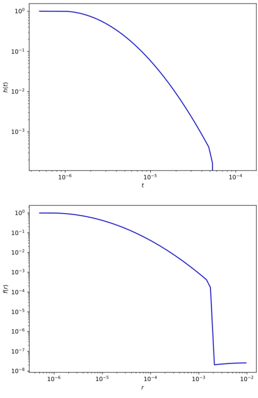
from 08/14/2019 to 02/09/2020. Here the red number represents the count of repetitive crimes at the same location. The underlying map is from OpenStreetMap. 7 1.4 Temporal (top) and spatial (bottom) triggering effects’ decay functions for all
crimes in Los Angeles from 2009 to 2014. Here r is distance (in degrees) and
t is time (in days). The decay functions are estimated using the multivariate spatiotemporal Hawkes process in [YSB19] with nonparametric kernels. Note that the drop in f(r) when r is between 0.001 and 0.01 might be due to the artifact of our model such as the choice of the support. . . 8 1.5 Mutual-triggering effects between different kinds of crimes estimated via the
model in [YSB19]. Lighter color represents a stronger trigger effect. The crime types are (from 0 to 11) other, theft, grand theft auto, vandalism, burglary/theft from motor vehicle, robbery, burglary, aggravation, homicide, grand theft person, arson, and kidnap. . . 9
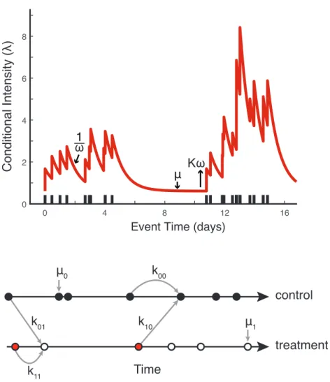
2.1 Self-exciting point-process models capture the dynamics of gang violent crime events. A temporal self-exciting point-process modelλ(t) =µ+P
ti<tKg(t−ti)
with exponential kernelg(t) =ωe−ωt(Top). Non-retaliatory gang crimes assigned to each condition arise spontaneously at rate µj. Retaliations assigned to each condition may be triggered through separate pathways (Bottom). The parame-ter kij is an estimate of the average number of retaliations of type j triggered by a single crime of type i. The parameters k11 and k01 link previous crimes
assigned to the treatment and baseline interventions, respectively, to retaliations subsequently assigned to the treatment intervention. The parameters k00 and
k10link previous crimes assigned to the baseline and treatment interventions,
re-spectively, to retaliations subsequently assigned to the baseline intervention. If treatment interventions (red events) reduce the risk of gang retaliation, then we expect k11 < k01 and k10< k00. . . 16
2.2 Spatiotemporal point process intensities of gang crimes in South Los Angeles. (A). The log of background intensity function µfor gang violent crimes mapped over space. (B) Contour plot of the density of background gang aggravated assaults and homicides determined by declustering. (C) Point locations of background gang aggravated assaults and homicides determined by declustering. (D) The log of spatiotemporal self-excitation of retaliation λ−µ mapped over space. (E) Contour plot of the density of retaliatory gang aggravated assaults and homicides determined by declustering. (F) Point locations of retaliatory gang aggravated assaults and homicides determined by declustering. Boundaries for ten GRYD IR Zones [BSY17] in South Los Angeles are outlined in black. . . 19
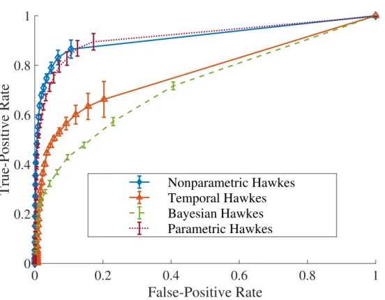
3.1 Model comparison using synthetic networks. We show the mean ROC curves with error bars (averaged over ten simulations, each with a different triggering matrix) on edge reconstruction. The ROC curve of a better reconstruction should be closer to 1 for a larger range of horizontal-axis values, such that it has a larger area under the curve (AUC), which is equal to the probability that a uniformly-randomly chosen existing edge in a ground-truth network has a larger weight than a uniformly-randomly chosen missing edge in the inferred network. . . 39 3.2 Model comparison using synthetic networks: Inferred (left) temporal and (right)
spatial kernels using three different methods: Temporal Hawkes, Parametric Hawkes, and Nonparametric Hawkes. The dashed curves are (ground-truth) ker-nels that we used to generate the synthetic data. . . 41 3.3 ROC curves of four different Hawkes models for reconstructing three Gowalla
friendship networks. We show results for Nonparametric Hawkes (blue dashed curves), Temporal Hawkes (yellow dash-dotted curves), Bayesian Hawkes (red solid curves), and Parametric Hawkes (dotted purple curves). . . 43 3.4 Three different friendships networks in the Gowalla data set. We compare
differ-ent network-reconstruction methods for these networks. . . 46 3.5 Crime-topic networks generated by the Nonparametric Hawkes and Temporal
Hawkes methods colored by community assignments from modularity maximiza-tion (from left to right): Nonparametric Hawkes in Westwood, Temporal Hawkes in Westwood, Nonparametric Hawkes in Wingfoot, and Temporal Hawkes in Wingfoot. . . 47 3.6 All possible three-node motifs for a network of events in the form of a directed
acyclic graph (DAG). The DAG structure arises from the temporal information in the events. We highlight the nodes in the feedforward-loop motif (D) in red. 51
4.1 The estimation results of STHC on U = 1 data. Ground-truth spatial triggering densityf(r) as red triangles and estimated triggering density as blue circles (left). Temporal triggering densityh(t) as red triangles and estimated triggering density as blue circles (right). . . 67 4.2 Ground-truthK matrix, STHC (the first row, from left to right), NPHC and EM
estimation results (the second row, from left to right). . . 68 4.3 Ground-truth K matrix, STHC, NPHC and EM estimation results (from left to
right). . . 69 4.4 The estimation results of STHC onU = 10 data. Ground-truth spatial triggering
densityf(r) as red triangles and estimated triggering density as blue circles (left). Temporal triggering densityh(t) as red triangles and estimated triggering density as blue circles (right). . . 70 4.5 The estimation results of STHC on U = 10 data with a Pareto triggering density
in time, a uniform triggering density in time (the first row, from left to right), a power-law triggering density in space and a uniform triggering density in space (the second row, from left to right). Ground-truth spatial triggering density f(r) as red triangles and estimated triggering density as blue circles. . . 71 4.6 The estimation results of STHC on U = 10 data with a Pareto triggering density
in time, a uniform triggering density in time (the first row, from left to right), a power-law triggering density in space and a uniform triggering density in space (the second row, from left to right). Ground-truth temporal triggering density
h(t) as red triangles and estimated triggering density as blue circles. . . 72 4.7 ROC curves of different methods (STHC, NPHC and EM) on subnetworks in
Gowalla and Brightkite data sets. The dashed line (red) is from random guess. . 76 4.8 Friendship network reconstruction using different methods on Brightkite-SD. Here
4.9 Estimated spatial triggering densities for Brightkite-SD, Gowalla-CHI (the first row, from left to right), Brightkite-LA, and Gowalla-SF (the second row, from left to right). The plot is in the log-log scale and we normalize the triggering density for easy comparison. Note that the drop in f(r) when r is between 0.0001 and 0.001 might be due to the artifact of our model such as the choice of the support for triggering densities. . . 78 4.10 Estimated temporal triggering densities for Brightkite-SD, Gowalla-CHI (the first
row, from left to right), Brightkite-LA, and Gowalla-SF (the second row, from left to right). The plot is in the log-log scale and we normalize the triggering density for easy comparison. . . 79 5.1 Visual illustration of our spatial point-process model via VAE. The spatial events
or embeddings X are fed into a neural network with parameter φ to get the mean and variance for the approximate posterior qφ(z|X), which is then used to calculate the KL divergence term. We can generate samples from the posterior using the reparameterization trick with from a standard normal distribution. Then the sample z is fed into a neural network with parameter θ to obtain f(z), which combining with the events X and kernel Kσ yields the intensity function
λ. Finally, we get the loss function from the KL term and the likelihood function from λ. . . 87 5.2 Estimated density functions for a Gowalla user in NYC (log scale). The first row
from left to right: observed check-in locations (in red), held-out check-in locations (in blue, as missing data) and the estimated intensity from VAE-SPP. The second row from left to right: the estimated intensity (or density) from VAE-CF, KDE and TGCP. . . 95
6.1 Overview of the system for early warning of opioid spikes. The initial overdose toxicology report shows fentanyl, benzodiazepine, and heroin present. Each drug is vectorized using SMILES and the event belongs to an overdose category using spectral clustering based on earth mover’s distance of the drug vectors (“drug movers’ distance”). The increase in the intensity of the Hawkes process is de-termined by the category and it allows for the prediction of an opioid overdose spike, triggered in the branching process by the initial overdose. . . 100 6.2 An illustration for an initial event and its triggered events in one of the categories
(i.e. one of the Hawkes processes). The initial overdose event marked in triangle symbol consists of four drug substances and it triggered four neighboring events consisting of different drug substances. . . 101 6.3 Flow chart of the algorithm. The spatiotemporal events are fed into a multivariate
Hawkes process to obtain the graph of zip codes. The graph is then used in GSRNN with two LSTM networks and a fully connected layer. . . 102 6.4 Inferred versus exact hourly crime rates for Chicago (left) and Los Angeles (right)
LIST OF TABLES
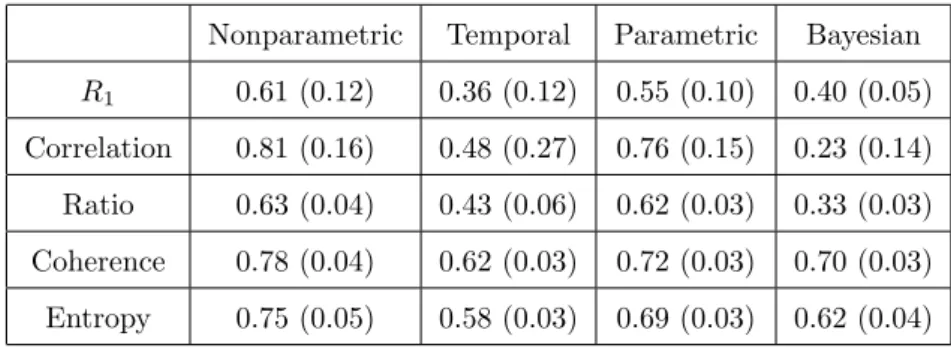
2.1 Notation. . . 22 3.1 Reciprocity of the triggering matrices that we infer using different methods: a
nonparametric spatiotemporal Hawkes model, a temporal Hawkes model, a para-metric spatiotemporal Hawkes model, and a fully Bayesian Hawkes model. We report the mean and standard deviation (in parentheses) over ten simulations that use the same (ground-truth) triggering matrix. . . 37 3.2 Reciprocity of the triggering matrices that we infer using different methods: a
nonparametric spatiotemporal Hawkes model, a temporal Hawkes model, a para-metric spatiotemporal Hawkes model, and a fully Bayesian Hawkes model. We report the mean and standard deviation (in parentheses) over ten simulations, each with a different (ground-truth) triggering matrix. . . 37 3.3 The L1 errors of the inferred spatial and temporal kernels. We simulate ten
point processes with the same triggering matrix and triggering kernel. We report the mean and standard deviation (in parentheses) of the L1 errors averaged over
ten simulations that use the same triggering kernel and matrix. Note that the exclusively temporal model does not estimate a spatial kernel. . . 40 3.4 Normalized mutual information (NMI) between the outputs of different
community-detection methods applied to the inferred networks (from four different types of Hawkes models) and the ground-truth community structure (averaged over ten simulations, each with a different triggering matrix). . . 42 3.5 Mean NMI (with one standard deviation reported in parentheses) between
com-munity assignments from several comcom-munity-detection methods and the classi-fications from [KBB17] in the 100 neighborhoods in Los Angeles with the most recorded crime events between 1 January 2009 and 19 July 2014. . . 48
3.6 Comparison of our stochastic declustering results for the Nonparametric Hawkes, Parametric Hawkes, and Temporal Hawkes methods using synthetic point-process data with networks from a WSBM (see section 3.3.1) and background labels from the simulation from algorithm 3. (We do not include results for Bayesian Hawkes, because it does not provide P directly.) We report the mean and the standard deviation (in parentheses) of the branching-ratio error, precision, and recall over ten simulations (which we do for ten point processes with the same triggering kernels and matrix). For each simulation, each calculation is the mean over 20 runs of stochastic declustering. . . 50 4.1 The computation time for different methods on synthetic data sets. Here the
time is in seconds. . . 69 4.2 Error measures for STHC on U = 10 data sets with different triggering densities. 70 4.3 The computation time for different methods on Gowalla and Brightkite data sets.
Here the time is in seconds. . . 79 5.1 Testing results on the simulation data sets. Both the mean and standard
deriva-tion (in parentheses) are percentages. . . 93 5.2 Testing results on the Gowalla data sets with uniform grids. Both the mean and
standard derivation (in parentheses) are percentages. . . 94 5.3 Testing results on the Gowalla data sets without discretization. Both the mean
and standard derivation (in parentheses) are percentages. . . 94 5.4 Testing results on the MovieLens data sets. . . 96 5.5 Testing results on MovieLens-100K. These methods share the same network and
are trained with 100 epochs. The test data are used to evaluate the model with the best performance during the validation. VAE-SPP-Separate means that GNN is trained separately with VAE-SPP. . . 98
ACKNOWLEDGMENTS
I would like to pay special regards to my advisor, Andrea Bertozzi, for her guidance through each stage of the process. She has always been helpful from my undergraduate summer research project to the writing of this thesis. Without her kindness and invaluable assistance, it would have been impossible for me to finish this rewarding Ph.D. journey. I would like to show my gratitude to the other committee members for all of their persistent help during many of my projects: P. Jeffrey Brantingham for sharing data and contributing ideas about crime as a social scientist, Mason A. Porter for introducing ideas in network science and for giving writing suggestions, and Wotao Yin for helping me with the model optimization. I wish to thank all the collaborators whose assistance was a milestone in the completion of each of these projects. I would like to pay special regards to Frederic (Rick) Paik Schoenberg for his great advice throughout my study. I would like to also acknowledge the support and great love from my family and friends, my girlfriend Candice, my mother Haifeng, my father Jianchun, and the many Ph.D. students in our program. They kept me deeply motivated and this thesis would not have been achievable without their help.
Chapter 3 includes Multivariate Spatiotemporal Hawkes Processes and Network Recon-struction [YLB19] by Baichuan Yuan, Hao Li, Andrea L. Bertozzi, P. Jeffrey Brantingham, and Mason A. Porter, SIAM J. Math. Data Sci 1.2 (2019): 356–382, DOI:10.1137/18M1226993. BY contributed to the derivation of algorithms, simulation methods, and numerical exper-iments. HL helped to evaluate simulation data and real-world applications. ALB helped with examples and many suggestions. PJB helped to interpret results related to crime. MAP helped with ideas from network science and writing suggestions. All authors assisted with manuscript preparation.
Chapter 4 containsFast Estimation of Multivariate Spatiotemporal Hawkes Processes and Network Reconstruction [YSB19] by Baichuan Yuan, Frederic (Rick) Paik Schoenberg and Andrea L. Bertozzi, submitted. BY developed the inference approach and run numerical experiments. FPS helped with the consistency proof and the design of experiments. ALB helped with ideas in L2 regularization and many suggestions. All assisted in manuscript
preparation.
Chapter 5 contains Variational Autoencoders for Highly Multivariate Spatial Point Pro-cesses Intensities [YWM20] by Baichuan Yuan, Xiaowei Wang, Jianxin Ma, Chang Zhou, Andrea L. Bertozzi and Hongxia Yang, accepted by the International Conference on Learn-ing Representations, 2020. BY contributed to the algorithm formulation, proofs, numerical experiments, and writing. XW helped with figures, the notation table, and writing. JM and CZ provided expertise on variational inference and recommender systems. ALB helped with numerous suggestions on research and writing. HY helped with the problem formulation and writing.
Chapter 6 contains two application papers: Graph-based deep modeling and real-time forecasting of sparse spatiotemporal data[WLZ18] by Bao Wang, Xiyang Luo, Fangbo Zhang, Baichuan Yuan, Andrea L. Bertozzi, and P. Jeffery Brantingham, KDD MiLeTS workshop, 2018. BW, XL, and FZ contributed equally to the algorithm and numerical experiments. BY contributed the point process part. PJB helped with crime data and insights about the results. ALB helped with many suggestions on the problem formulation and paper structure. All authors assisted with manuscript preparation; SOS-EW: System for Overdose Spike Early Warning using Drug Mover’s Distance-based Hawkes Processes [CYL19] by Wen-Hao Chiang, Baichuan Yuan, Wen-Hao Li, Bao Wang, Andrea L. Bertozzi, Jeremy Carter, Brad Ray, and George Mohler, ECML-PKDD SoGood Workshop, 2019. WC and BY contributed equally to the model design and experiments. HL and BW helped with data preprocessing. ALB helped with many suggestions on the project and writing. JC and BR provided data and helped with writing. GM helped to guide the research project and run numerical experiments. I truly appreciate the fellowship from the National Institute of Justice. NIJ Fellowship 2018-R2-CX-0013 provided essential support for my last two years in school in order to finish this thesis.
VITA
2015 B.S. (Mathematics and Applied Mathematics), Zhejiang University, China 2015–2018 Graduate Research Assistant, Department of Mathematics, UCLA.
2018–2020 National Institute of Justice Graduate Research Fellow, Department of Mathematics, UCLA.
PUBLICATIONS
Baichuan Yuan, Frederic P. Schoenberg, Andrea L. Bertozzi. Fast Estimation of Multivariate Spatiotemporal Hawkes Processes and Network Reconstruction. Submitted.
Baichuan Yuan, Xiaowei Wang, Jianxi Ma, Chang Zhou, Andrea L. Bertozzi, Hongxia Yang. Variational Autoencoders for Highly Multivariate Spatial Point Processes Intensities, accepted to International Conference on Learning Representations (ICLR), 2020.
Baichuan Yuan, Hao Li, Andrea L. Bertozzi, P. Jeffrey Brantingham, and Mason Porter, Multivariate Spatiotemporal Hawkes Processes and Network Reconstruction, SIAM J. Math-ematics of Data Science, 1(2), pp. 356–382, 2019.
Baichuan Yuan, Yen Joe Tan, Maruti K. Mudunuru, Omar E. Marcillo, Andrew A. Delorey, Peter M. Roberts, Jeremy D. Webster, Christine N. L. Gammans, Satish Karra, George D. Guthrie, Paul A. Johnson; Using Machine Learning to Discern Eruption in Noisy Envi-ronments: A Case Study Using CO2-Driven Cold-Water Geyser in Chimay´o, New Mexico. Seismological Research Letters, 90 (2A): 591–603, 2019.
Wen-Hao Chiang*, Baichuan Yuan*, Hao Li, Bao Wang, Andrea Bertozzi, Jeremy Carter, Brad Ray, George Mohler; SOS-EW: System for Overdose Spike Early Warning using Drug Mover’s Distance-based Hawkes Processes. ECML-PKDD Workshop on Data Science for Social Good, 2019. (* equal contribution)
Bao Wang, Xiyang Luo, Fangbo Zhang, Baichuan Yuan, Andrea L Bertozzi, P Jeffrey Brantingham; Graph-Based Deep Modeling and Real Time Forecasting of Sparse Spatio-Temporal Data. KDD Workshop on Mining and Learning from Time Series, 2018.
Yonatan Dukler, Yurun Ge, Yizhou Qian, Shintaro Yamamoto, Baichuan Yuan*, Long Zhao, Andrea L. Bertozzi, Blake Hunter, Rafael Llerena, and Jesse T. Yen, Automatic decomposi-tion and mitral valve segmentadecomposi-tion of cardiac ultrasound time series data, Medical Imaging 2018: Image Processing. Vol. 10574. International Society for Optics and Photonics, 2018. (* corresponding author)
Baichuan Yuan, Sathya R Chitturi, Geoffrey Iyer, Nuoyu Li, Xiaochuan Xu, Ruohan Zhan, Rafael Llerena, Jesse T Yen, Andrea L Bertozzi, Machine Learning for Cardiac Ultrasound Time Series Data, Medical Imaging 2017: Biomedical Applications in Molecular, Structural, and Functional Imaging. Vol. 10137. International Society for Optics and Photonics, 2017.
Eric L. Lai*, Daniel Moyer*, Baichuan Yuan*, Eric Fox, Blake Hunter, Andrea L. Bertozzi, P Jeffrey Brantingham, Topic Time Series Analysis of Microblogs, IMA Journal of Applied Mathematics, 81(3) pp. 409-431, 2016. (* equal contribution)
CHAPTER 1
Introduction
Spatiotemporal (ST) point processes, especially ST-Hawkes processes (also known as “self-exciting point processes”1) have been widely used to model and forecast clustered
point-process data in the study of earthquakes [Oga98], crimes [MSB11], invasive species [BSM12], terrorist attacks [PW12], infectious diseases [Sch18], and financial markets [BMM15]. These models, which are characterized by a triggering density describing how the occurrence of one event may spark future events nearby, have real-world impacts on the crime rate in Los Angeles [MSM15].
Recently, digital devices such as smartphones and tablets generate a massive amount of spatiotemporal data on human activities, providing a wonderful opportunity for researchers to gain insight into human dynamics through our “digital footprints”. A wide variety of human activities are now analyzed using such data, creating new disciplines such as com-putational social science and digital humanities [LPA09]. Examples of such activities in-clude online check-ins in large cities [CML11], human mobility [BCG09] and currency flow [BHG06], online communications during Occupy Wall Street[CDF13], crime reports in Los Angeles county [KBB17], and many others. Spatiotemporal point processes [SBG14], as a class of generative models, can detect and explain lots of clustering effects from structural differences in space and time. In fig. 1.1, we visualize some examples of spatiotemporal clus-ters from the Twitter data in [LMY16]. To further incorporate accompanying information on each event such as the type of crime or the magnitude of an earthquake, multivariate point processes have been the subject of significant research in the areas of criminology [Moh14], finance [BMM15], neuroscience [CSS17], and text analysis [DFA15]. Applications
Figure 1.1: Spatiotemporal Twitter events in Los Angeles (LA) about the topic “outlets” and topic “Christmas”. The spatial and temporal clustering effects are clearly presented: events about “outlets” are spatially clustered around the location of the outlets and events about “Christmas” are temporally clustering around the Christmas day.
include network reconstruction [LA14, FSS16, HW16, YLB19, MRW18], causal inference [ABG17, EDD17, BYS18] and social-media cascade modeling [LMY16, FWR15]. The focus of this thesis is to provide a detailed review of current methods for multivariate ST point processes and their challenges when facing these new applications. Then we develop a set of approaches to bridge the gap between real-world applications and current methods.
1.1
Motivation
1.1.1 Social NetworksNetwork analysis is a powerful approach for representing and analyzing complex systems of interacting components [New18], and network-based methods can provide considerable insights into the structure and dynamics of complex spatiotemporal data [Bar18]. It has been valuable for studies of both digital human footprints and human mobility [BBG18]. To give one recent example, Noulas et al. [NSL12] studied geographic online social networks to illustrate similarities and heterogeneities in human mobility patterns.
Suppose that each node in a network represents an entity, and that the edges (which can be either undirected or directed, and can be either unweighted or weighted) represent spatiotemporal connections between pairs of entities. For instance, in a data set of check-ins on a social-media platform, one can model each user as a node, which has associated check-in time and locations. In this case, one can suppose that an edge exists between a pair of users if they follow each other on the platform. One can use edge weights to quantify the amount of “influence” between users, where a larger weight signifies a larger impact. In our investigation, we assume that the relationships between nodes are time-independent.2
Here we illustrate this idea via a fictional example in fig. 1.2, where nodes are users in a social-media network and an edge from node A to node B presents the influence of user A on user B. We further visualize the impact between users when they share posts over time on social media. In some cases, the entities and relationships are both known, and one can investigate the structure and dynamics of the associated networks. However, in many situations, network data are incomplete — with potentially a large amount of missing data, in the form of missing entities, interactions, and/or metadata [SSB11] — and it may not be possible to directly observe the relationships between nodes [SNM11]. For example, social-media companies attempt to infer friendship relationships between their users to provide accurate friendship recommendations for online social networks.
2Depending on the relative time scales between spatiotemporal processes and network dynamics, it may be important to consider time-dependent edges [PG16, Hol15].
Figure 1.2: Top: a social network represents the influence between users in a fictional social media. Note that user E is not affected by any user. Bottom: Post-sharing timeline for each user. Here the line edge represents the triggering effect of one user’s sharing on other users and the curved edge represents the self-excitation within each user. User E, not influenced by other users, displays an almost uniform distribution of sharing events.
In the last few years, there has been a considerable effort on inferring missing data (both the structure and weight) in networks. A basic approach for inferring relationships among entities is to calculate cross-correlations of their associated time series [Lau96]. Another ap-proach is to use coefficients from a generalized linear model (GLM) [NW72], a generalization of linear regression that allows response variables to have a non-Gaussian error-distribution. Recently, researchers have begun to use point-process methods [SJ10] in network recon-struction. For example, Perry and Wolfe [PW13] modeled networks as multivariate point processes and then inferred covariate-based edges (both their existence and their weights). As a well-studied family of point-process models, Hawkes processes have been employed of-ten for studying human dynamics [LA14, FSS16]. Hawkes-process models are characterized by mutual “triggering” among events [Oga88], as one event may increase the probability for subsequent events to occur. Such models can capture inhomogeneous inter-event times and causal (temporal) correlations, which are important considerations for human dynamics [KP15]. These properties illustrate the relevance of using Hawkes processes in social-network applications [KJK18]. It thus seems promising to employ such processes for network infer-ence on dynamic human data, such as crime events and online social media. For example, Linderman and Adams [LA14] proposed a fully Bayesian Hawkes model that they reported to be more accurate at inferring missing edges for their data than GLMs, cross-correlations, and a simple self-exciting point process with an exponential kernel. However, the aforemen-tioned temporal point-process models are not without limitations. For example, most of these models do not use spatial information, even when it plays a significant role in a sys-tem’s dynamics. Furthermore, many studies assume an a priori model [LA14] or a specific parametrization [CGB14] for their point processes.
1.1.2 Crime Forecasting
Recent years have seen a surge of complete criminal records and related information collected by law enforcement. In Los Angeles, for example, there are nearly half-million criminal records collected by the Los Angeles Police Department (LAPD). The volume of data com-bined with the development of quantitative techniques has boosted crime forecasting, which
helps to prevent crime and evaluate police intervention. Mohler et al. [MSM15] reported a 7.4% reduction in crime when the police department used their point-process model for daily patrol.
Current models on crime prediction usually focus on certain desired properties of pre-dictive policing models. Crime hotspots describe crimes’ spatial distribution using kernel density estimation or using spatial point processes. These models are easy to compute and can incorporate covariates such as demographics [WB12]. As a result, they are scalable to multivariate data. However, the standard model for crime hotspots is static in time and multiple timescales are usually not reflected [Moh14].
To model the dynamics of hotspots, self-exciting point-process models adapted from seis-mology [MSB11] assume near-repeats of crimes [HR12] and the decay of risk along time and spatial neighborhood. In fig. 1.3, we illustrate the near-repeat phenomenon via visualizing recent burglaries. The decay functions over time and space estimated via the point-process model in [YSB19] are showed in fig. 1.4. This model is extended as a marked point-process model to include covariates, such as crime type [Moh14] and spatial features [RG18]. Marked point-process models, especially multivariate models, are able to reveal the mutual-triggering effects between different crime types as showed in fig. 1.5. The inference of these models is based on maximizing the log-likelihood function using off-the-shelf optimization techniques such as BFGS, or expectation maximization (EM) algorithm [VS08]. In terms of algorithm complexity, each evaluation of the log-likelihood function isO(N2) and the overall
complex-ity for EM isO(N3) where N is the number of crime events. This is not ideal when handling
millions of crimes in the data set
Accurate spatiotemporal events forecasting is also one of the important tasks for artificial intelligence. Recent developments in the deep neural network provide multiple tools for crime forecasting. Kang et al. [KK17] utilized a convolutional neural network (CNN) to extract the features from historical crime data, and then used a support vector machine (SVM) to classify whether there will be a crime or not at the next time slot. CNN-based approaches are scalable for large data sets and have good generalization ability. The data at a certain timescale are represented by the spatial distribution histogram on the grid and a CNN is used
Figure 1.3: Recent burglary crimes from LAPD’s Crime Mapping in part of Santa Monica from 08/14/2019 to 02/09/2020. Here the red number represents the count of repetitive crimes at the same location. The underlying map is from OpenStreetMap.
10 6 10 5 10 4 t 10 3 10 2 10 1 100 h( t) 10 6 10 5 10 4 10 3 10 2 r 10 8 10 7 10 6 10 5 10 4 10 3 10 2 10 1 100 f(r )
Figure 1.4: Temporal (top) and spatial (bottom) triggering effects’ decay functions for all crimes in Los Angeles from 2009 to 2014. Here r is distance (in degrees) and t is time (in days). The decay functions are estimated using the multivariate spatiotemporal Hawkes process in [YSB19] with nonparametric kernels. Note that the drop inf(r) whenris between 0.001 and 0.01 might be due to the artifact of our model such as the choice of the support.
Figure 1.5: Mutual-triggering effects between different kinds of crimes estimated via the model in [YSB19]. Lighter color represents a stronger trigger effect. The crime types are (from 0 to 11) other, theft, grand theft auto, vandalism, burglary/theft from motor vehicle, robbery, burglary, aggravation, homicide, grand theft person, arson, and kidnap.
to predict the future histogram. This CNN-based approach is sub-optimal from two aspects. First, the geometry of a city is usually highly irregular, resulting in the city’s configuration taking up only a small portion of its bounding box. This introduces unnecessary redundancy into the algorithm. Second, spatial sparsity can be exacerbated by the spatial grid structure. Directly applying a CNN to fit the extreme sparse data will lead to all zero weights due to the weight sharing of CNNs [WYB19]. This can be alleviated by using spatial super-resolution, with an increased computational cost. Moreover, this lattice-based data representation omits geographical information and spatial correlations within the data itself.
1.2
Directions for Improvement
To improve the effectiveness of ST point processes, a natural question to ask is what makes a good point-process model for applications above. Given the size of the data, scalable methods are essential for real-time forecasting and evaluation. Moreover, real-world data sets contain rich information aside from spatiotemporal stamps. For example, for criminal records, we want to use information such as gang involvement, a brief description of the crime, and intervention attempts. As a result, a multivariate representation of the events is useful in modeling and can utilize additional data. Finally, in forecasting problems, the ability to generalize the algorithm is ideal since we are more interested in events that we have not seen yet. In summary, a better point-process model should be able to handle large-scale multivariate data in real-time and achieve reliable results in new data. Current methods all have limits in some respects. In this thesis, we propose new approaches to achieve these three properties, including scalability, generalization ability as well as the use of the multivariate model. Multivariate models will be able to analyze millions of data in linear time O(n) to achieve real-time prediction.
Our models relieve the computational burden of point-process models and make it pos-sible to apply them on multiple large-scale problems such as network reconstruction, rec-ommendation systems and predictive policing. For example, a real-time and accurate crime forecasting model will improve the design of police patrol. Applications of our model are not
limited to these directions. Retaliation has been long featured in the discussion of gangs, rising almost to one of de facto definitive characteristics [Pap09]. During the collabora-tion with the City of Los Angeles Mayor’s Office of Gang Reduccollabora-tion & Youth Development (GRYD), we discovered a promising application [BSY17] of multivariate point processes on the evaluation of GRYD’s gang intervention program in terms of causal effects. In the case of missing data in crime records, our multivariate approach has been applied to crime network inference [YLB19] and gang retaliatory dynamics [BYS18].
CHAPTER 2
Background
2.1
A Brief Review of Point Processes
Given a complete, separable metric space, apoint process S is a random measure that values in {0,1,2, . . .} ∪ {∞} [SBG14]. While the definitions and results below can be extended quite readily to other metric spaces, we will assume for simplicity that the metric space is a bounded interval [0, T] in time or a bounded area R×[0, T] in space-time.
We first consider a temporal point process, which consists of a list {t1, t2, . . . , tN} of N time points, with corresponding events 1,2, . . . , N. Let S[a, b) denote the number of points (i.e. events) that occur in a finite time interval [a, b), with a < b. One typically models the behavior of a simple temporal point process (multiple events cannot occur at the same time) by specifying its conditional intensity functionλ(t), which represents the rate at which events are expected to occur around a particular time t, conditional on the prior history of the point process before time t. Specifically, when Ht = {ti|ti < t} is the history of the process up to time t, one defines the conditional intensity function
λ(t) = lim
∆t↓0
E[S[t, t+ ∆t)|Ht]
∆t .
One important point-process model is a Poisson process, in which the number of points in any time interval follows a Poisson distribution and numbers of points in disjoint sets are independent of each other. A Poisson process is called homogeneous if λ(t)≡constant, and it is thus characterized by a constant rate at which events are expected to occur per unit time. It is called inhomogeneous if the conditional intensity function λ(t) depends on the time t (e.g. λ(t) =e−t). In both situations, numbers of points (i.e. events) in disjoint intervals are independent random variables.
We now discuss self-exciting point processes, which allow one to examine a notion of causality in point-process models. If we consider a list {t1, t2, . . . , tN} of time stamps, we say that a point process is self-exciting if
Cov [S(tk−1, tk), S(tk, tk+1)]>0, with tk−1 < tk< tk+1,
where k is a positive integer. In a self-exciting point process, if an event occurs, another event becomes more likely to occur locally in time.
A univariate temporal Hawkes process, which we express using the common cluster rep-resentation [HO74], has the following conditional intensity function:
λ(t) =µ(t) +KX
tk<t
g(t−tk), (2.1)
where the background rate µ(t)> 0 can either be a constant or a time-dependent function that describes how the likelihood of some processes (crimes, e-mails, tweets, and so on) evolves in time. For example, violent crimes are more likely to occur at night than during the day, and business e-mails are less likely to be sent during the weekend than on a weekday. One can construe the rate µ(t) as a process that designates the likelihood of an event to occur, independent of the other events. The summation term in eq. (2.1) describes the self-excitation: past events increase the current conditional intensity. The function g(t) ≥ 0 is called the triggering density or triggering kernel satisfying R∞
0 g(v)dv = 1, which describes
the conductivity of events, and the productivity parameter K denotes the mean number of events that are triggered by an event, which is typically required to satisfy 0 ≤ K < 1 in order to ensure stationarity and subcriticality [Haw71]. One standard example is a Hawkes process with an exponential kernel g(t) = ωe−ωt, where the constant decay rate ω for the triggering kernel controls how fast the rate λ(t) returns to its baseline level µ(t) after an event occurs.
We fit the Hawkes process above to gang aggravated assaults and homicides in South Los Angeles from 2014–2015 in fig. 2.1 (A). Two cycles of gang violent crimes occur within a period of eighteen days. The conditional intensity λ reflects the instantaneous rate of gang crime. The background rateµis the expected rate of gang crime in the absence of retaliation.
A crime causes λ to jump by an amount Kω, increasing the risk of retaliation. The risk of retaliation following a single crime decays exponentially with a rate ω and a mean lifetime of 1/ω. We expect violence interruption deployed in the aftermath of a crime to cause the conditional intensity to fall and therefore future crimes to be less likely to occur than in the absence of intervention.
2.1.1 Multivariate Temporal Models
In a multivariate temporal point process, there are U different point processes (Su)u=1,...,U; and the corresponding conditional intensity functions are (λu(t))u=1,...,U. We seek to infer the intensity functions from observed data (tj, uj)j=1,...,N in a time window [0, T], where tj and
uj, respectively, are the time and point-process indices of event j. There are numerous ap-plications of temporal multivariate point processes; they include financial markets [BMM15], real-time crime forecasting [WLZ18], and neuronal spike trains [BKM04].
Let’s first consider two examples of multivariate processes that are not self-exciting. A trivial example of a multivariate point process is the multivariate Poisson process, in which each point process is a univariate Poisson process. Another example is the multivariate Cox process, which consists of doubly stochastic Poisson processes (so the conditional intensity itself is a stochastic process). Perry and Wolfe [PW13] used a Cox process to model e-mail interactions (edges) among a set of users (nodes).
Instead of modeling edges as Cox processes, Fox et al. [FSS16] used multivariate Hawkes processes to model people (nodes) communicating with each other via e-mail. Their condi-tional intensity function has an exponential kernel and a nonparametric background function
µu(t)≥0 for each person (process) u. It is written as
λu(t) = µu(t) +
X
ti<t
Kuiuωe
−ω(t−ti), (2.2)
whereKuv ≥0 is the expected number of events of personv that are triggered by one event of person u.
of temporal point processes indexed byu= 1, ..., U, where each subprocessNuhas conditional intensity λu(t) = µu + X tk<t Kuk,uguk(t−tk). (2.3)
The idea behind this formula is that the triggering density guk and productivity Kuk,u may
depend on the index of the point tk. Here µu is the background rate, indicating the rate at which points of markuoccur, absent any other prior events. For simplicity, one traditionally assumes a uniform background rate in time. K ∈RU×U is the triggering matrix, where Ku,v is the expected number of events of indexv that are triggered by one event of indexu. This triggering effect, in this temporal-only case, is closely related to Granger causality [Gra69]. In fact, subprocess u does not Granger-cause subprocess v if and only if Ku,v = 0 [EDD17]. Similarly, for stationarity and subcriticality, K needs to satisfy kKk < 1, where kKk is the spectral norm of K. We show an example of fitting the gang crime data above to this multivariate model in fig. 2.1 (B). Gang crimes assigned to two different intervention conditions are modeled as two interacting point processes.
2.1.2 Spatial Point Processes
While the major theory of point processes centers around the temporal dynamics, spatial point process (SPP) models [Dig83] are established in forestry and seismology, focusing on the stationary and isotropic case. We define the (first-order) intensity function λ(x), which is the expected rate of the accumulation of points around a particular spatial locationx. We write
λ(x) = lim |∆x|↓0
E[S(∆x)]
|∆x| , (2.4)
where ∆x is a small ball in the metric space, e.g. the Euclidean spaceRn, with the centre x and measure |∆x|. The second-order intensity function is naturally defined as
λ(2)(x, y) = lim
|∆x|,|∆y|↓0
E[S(∆x)S(∆y)]
|∆x||∆y| , (2.5)
measuring the chance of points co-occurring in both ∆x and ∆y. Normalizing this leads to the pair-correlation function g(x, y) = λ(2)(x, y)/λ(x)λ(y). Then g(x, y) > 1 indicates that
k11 k00 k10 k01 Time control treatment μ0 μ1 0 4 8 12 16
Event Time (days)
0 2 4 6 8 Conditional Intensity ( λ) Kω μ ω1
Figure 2.1: Self-exciting point-process models capture the dynamics of gang violent crime events. A temporal self-exciting point-process modelλ(t) =µ+P
ti<tKg(t−ti) with
expo-nential kernel g(t) = ωe−ωt (Top). Non-retaliatory gang crimes assigned to each condition arise spontaneously at rate µj. Retaliations assigned to each condition may be triggered through separate pathways (Bottom). The parameter kij is an estimate of the average num-ber of retaliations of type j triggered by a single crime of type i. The parameters k11 and
k01 link previous crimes assigned to the treatment and baseline interventions, respectively,
to retaliations subsequently assigned to the treatment intervention. The parametersk00 and
k10 link previous crimes assigned to the baseline and treatment interventions, respectively,
to retaliations subsequently assigned to the baseline intervention. If treatment interventions (red events) reduce the risk of gang retaliation, then we expect k11< k01 and k10< k00.
Common models in SPPs include the Poisson process with a non-stationary rateλ(x), and the Cox process with a nonnegative-valuedintensity process Λ(x), which is also a stochastic process. Cox processes conditional on a realization of the intensity process Λ(x) =λ(x) are Poisson processes with intensity λ(x). To model the aggregated points patterns, Poisson cluster (Neyman–Scott) processes generate parent events from a Poisson process. Then each parent independently generates a random number of offspring. The relative positions of these offspring to the parent are distributed according to some p.d.fKσ(x) in space [Dig83]. Many point-process models, including most Cox processes, are in fact Poisson cluster processes. The duality between Cox processes and cluster processes is widely used to construct Cox process models. For example, the kernel-based intensity process Λ(x) =P∞
i=1Kσ(x−xi) with
xi from a Poisson process, is essentially a Poisson cluster process. The number of offspring is from a Poisson distribution with λ = 1 and the relative position distribution is Kσ(x). Repulsive SPPs, on the other hand, model that nearby points of the process tend to repel each other. Higher-order intensities are often considered in this case, such as determinantal point processes.
Alternatively, if we are more interested in the realization intensityλ(x) than the mechan-ical interpretation, the trans-Gaussian Cox process provides a tractable way to construct the Cox process using a nonlinear transformation on a Gaussian process. Popular choices for Λ(x) include the log-Gaussian Cox process (LGCP) and the permanental process. Recent pa-pers on Cox processes have been extensively focused on the cases that are modulated via the Gaussian random field, due to its capability in modeling the intensity and pair-correlations between subprocesses. We aim to develop a more explicit approach to model interactions for fast inference and the generalization ability for new subprocesses.
2.1.3 Spatiotemporal Point Processes
Many real-world data sets include not only timestamps but also accompanying spatial infor-mation, which can be particularly important for correctly inferring and understanding the dynamics associated with such data [Bar18]. In earthquakes, for example, most aftershocks
usually occur geographically near the mainshock [Oga98]. In online social media, if two peo-ple often check-in at the same location at closely proximate times, there is more likely to be a connection between them than if such “joint check-ins” occur rarely [CML11]. These sit-uations suggest that it is important to examine spatiotemporal point processes, rather than just temporal ones. Indeed, there are myriad applications of spatiotemporal Hawkes pro-cesses, including crime forecasting [MSB11], the detection of anomalous seismicity [Oga98], and inference of Twitter topics [LMY16].
We characterize a spatiotemporal point process S(t, x, y) via its conditional intensity
λ(t, x, y), which is the expected rate of the accumulation of points around a particular spatiotemporal location. Given the historyHt of all points up to time t, we write
λ(t, x, y) = lim ∆t,∆x,∆y↓0 E[S{(t, t+ ∆t)×(x, x+ ∆x)×(y, y+ ∆y)}|Ht] ∆t∆x∆y .
For the purpose of modeling earthquakes, Ogata [Oga98] used a self-exciting point process with a conditional intensity of the form
λ(t, x, y) =µ(x, y) +KX
t>ti
g(x−xi, y−yi, t−ti).
In this setting, if an earthquake occurs, aftershocks are more likely to occur locally in time and space. The choice of the triggering kernel g(t, x, y) is inspired by physical properties of earthquakes. For example, Ogata [Oga98] used a modified Omori formula (a power law) [Oga88] to describe the frequency of aftershocks per unit time. In sociological applications, there is no direct theory to indicate appropriate choices for the kernel function. Some re-searchers have chosen specific kernels (e.g. exponential kernels) that are easy to compute. For example, Tita et al. [CGB14] used a spatiotemporal point process to infer missing infor-mation about event participants. They modeled interactions between event participants as a combination of a spatial Gaussian mixture model and a temporal Hawkes process with an exponential kernel. A key problem is how to justify kernel choices in specific applications. Another benefit of point-process modeling is that we can distinguish the clustering effects from the background or triggering via declustering. See section 3.3.4 for more details on declustering. We fit the spatiotemporal point process above to gang crimes in South Los Angeles in fig. 2.2 and show the declustering result.
0 5 km
A
0 5 kmB
0 5 kmE
0 5 kmD
C
0 5 kmF
0 5 kmFigure 2.2: Spatiotemporal point process intensities of gang crimes in South Los Angeles. (A). The log of background intensity function µfor gang violent crimes mapped over space. (B) Contour plot of the density of background gang aggravated assaults and homicides determined by declustering. (C) Point locations of background gang aggravated assaults and homicides determined by declustering. (D) The log of spatiotemporal self-excitation of retaliation λ − µ mapped over space. (E) Contour plot of the density of retaliatory gang aggravated assaults and homicides determined by declustering. (F) Point locations of retaliatory gang aggravated assaults and homicides determined by declustering. Boundaries for ten GRYD IR Zones [BSY17] in South Los Angeles are outlined in black.
2.1.4 Model Inference
Inference methods for point processes are mainly based on the order statistics or likelihood function. The order statistics are often estimated nonparametrically, such as the kernel estimator [Dig85] of the intensity function. For the likelihood-based inference, we assume that one observes events X ={ti}Ni=1 of the underlying point process over the area R. The
log-likelihood for the point process with intensity λ(t) over a certain space R is
logp(X|Θ) = N X i=1 log(λ(ti))− Z R λ(t) dt . (2.6)
The integration term is the log void probability and can be viewed as a normalization term for the likelihood.
In the multivariate temporal point process case, one can estimate the set of parameters Θ by minimizing the negative log-likelihood function
−log(L(Θ)) =− N X k=1 log(λuk(tk)) + U X u=1 Z T 0 λu(t)dt , (2.7)
where log(x) denotes the natural logarithm ofx. Recall thatukis the point process associated with event k. There are several variants of the MLE for the multivariate Hawkes process. One is to add regularization terms to Equation eq. (2.7) to improve the accuracy of parameter estimation. Lewis and Mohler [LM11] used maximum-penalized likelihood estimation, which enforces some regularity on the model parameters, to infer Hawkes processes. Linderman et al. [LA14] added random-graph priors on K and developed a fully Bayesian multivariate Hawkes model. See [MRW18] for theoretical guarantees on inferring Hawkes processes with a regularizer. Another research direction is to speed up the parameter estimation of point-process models. For example, Hall et al. [HW16] tried to learn the triggering matrix K
via an online learning framework for streaming data. In a very recent paper, Achab et al. [ABG17] developed a fast moment-matching method (instead of using a likelihood-based method) to estimate the matrix K.
For Cox processes, the likelihood is the expectation over the Poisson likelihood above. It is difficult to directly integrate over the distribution of Λ. Monte Carlo methods [AMM09]
are commonly used to approximate the expectation. To improve the scalability of the expen-sive sampling, many methods such as variational inference [LGO15], Laplace approximation [WR06] and reproducing kernel Hilbert spaces [FTS17] are proposed.
2.2
Point Processes on Real-world Problems
Multivariate point-process models have a wide range of applications. In network recon-struction, for example, one seeks to infer the relationships (i.e. edges) and the strengths of such relationships (i.e. edge weights) among a set of entities (i.e. nodes). When modeling the relationships in a network, it is more appropriate to use a multivariate point process than a univariate one. To utilize covariates in a criminal record, we need to extend the univariate self-exciting point-process model [MSB11] to the multivariate setting. For crime applications, each process could represent different gangs, crime types, zip code areas or police intervention attempts. Via defining subprocesses as different entities, the multivariate model can be applied to crime forecasting, gang network inference as well as causality es-timation. Multivariate Hawkes processes are closely related to Granger causality (Granger, 1969). As a result, one can hypothesize that the mutual effect parameters Kuv can reflect real-world connections among different processes. For example, if each gang is a single point process, Kuv >0 implies crimes in gang u will lead to crimes in gangv.
In a previous point-process model of crime [RG18], every crime increases a local crime risk that decays exponentially in time and diffuses as a Gaussian distribution in space. To increase the generalization ability, one can use a model-independent approach [ML08] to avoid the selection of a specific decay function (kernel) for different applications. In this setting, the kernel is assumed to be a stepwise constant function and the values will be learned from real-world data. EM-type algorithms are widely used in the inference of point-process models. However, this approach is far from satisfying [Sch18]. A specific limit is computation complexity. EM has a O(N3) time complexity and a O(N2) storage
requirement, which is not acceptable for larger data sets. It is important to improve the scalability of the multivariate point-process model.
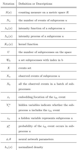
Table 2.1: Notation.
Notation Definition or Descriptions
S(x) counting measure on a metric spaceR
Nu the number of events of subprocessu
λu(x) intensity function of a subprocessu
Λu(x) intensity process of a subprocessu
Kσ(x) kernel function
U the number of subprocesses on the space
Ub a set subprocesses with index in b
X events set
Xu observed events of subprocessu
Xb all the observed events in a batch of
sub-processes
xi embedding/location of theithevent Yu
i hidden variables indicate whether the
sub-processuincludes theithevent
zu a hidden variable represents subprocessu
pu
i probability of theith event occurs in
sub-processu
φ, θ neural network parameters
Another application of multivariate models is the evaluation of a gang intervention pro-gram. Retaliation propels gang violence. Spontaneous attacks resulting from chance encoun-ters between rivals, or situational interactions that challenge gang territory or reputation can trigger cycles of tit-for-tat reprisals. Yet it has been difficult to determine if interventions that seek to reduce the likelihood of retaliation translate into lower rates of gang crime. One can use a multivariate spatiotemporal point process to quantify the magnitude of retaliation arising from gang crimes given two distinct types of post-event interventions. The methods are well-suited to the analysis of real-world interventions where there is an interaction be-tween outcomes. Our preliminary analysis [BSY17] of interventions in Los Angeles indicates that efforts to control rumors and engage impacted families, undertaken in the immediate aftermath of gang violent crimes, reduce the contagious spread of violence. These findings [BYS18, Wan18] have important implications for the design, implementation, and evaluation of gang violence prevention programs.
Finally, we want to clarify the difference between point-process models and time-series approaches. Point processes are generative models that are continuous in time. For time series analysis, however, it first discretizes the events into time bins and aggregates them together. We focus on the point-process models due to its convenient and natural represen-tation of crime and social media events with precise spatiotemporal stamps. We also worked on specific problems in seismology [YTM19] and medical imaging [YCI17, DGQ18], which are more appropriate for time-series methods.
CHAPTER 3
Multivariate Hawkes Processes and Network
Reconstruction
There is often latent network structure in spatial and temporal data, and the tools of net-work analysis can yield fascinating insights into such data. In this chapter, we propose a nonparametric and multivariate version of a spatiotemporal Hawkes process. Spatiotempo-ral Hawkes processes have been used previously to study numerous topics, including crime [MSB11], social media [LMY16], and earthquake forecasting [FSG16]. In our model, each node in a network is associated with a spatiotemporal Hawkes process. The nodes can “trigger” each other, so events that are associated with one node increase the probability that there will be events associated with the other nodes. We measure the extent of such mutual-triggering effects using a U ×U “triggering matrix” K, where U is the number of nodes. If one considers an exclusively temporal scenario, a point process udoes not “cause” (in the Granger sense [Gra69]) a point process v if and only if K(u, v) = 0 [EDD17]. Be-cause triggering between point processes reflects an underlying connection, one can try to recover latent relationships in a network fromK. Such triggering should decrease with both distance and time according to some spatial and temporal kernels. In this work, instead of assuming exponential decay [FSS16] or some other distribution [LA14, CGB14], we adopt a nonparametric approach [ML08] to learn both spatial and temporal kernels from data us-ing an expectation-maximization-type (EM-type) algorithm [VS08]. Recently, Chen et al. [CSS17] also studied Hawkes processes with a nonparametric approach, although they only considered exclusively temporal kernels.
This model helps fill a gap in the literature on incorporating spatial information into multivariate self-exciting point processes [Rei18a]. To our knowledge, it is the first method
that uses a multivariate spatiotemporal Hawkes process with a nonparametric method to estimate a triggering kernel. Inspired by the successful employment of spatiotemporal uni-variate Hawkes processes in earthquake forecasting [FSG16, ML08] and predictive policing [MSM15], our work extends these ideas to multivariate Hawkes processes and uses these ideas in an application to network reconstruction. We illustrate our approach using both syn-thetic networks and networks that we construct from real-world data sets (a location-based social-media network, a narrative of crime events, and violent gang crimes). Our approach outperforms other recent point-process network-reconstruction methods [FSS16, LA14] on both synthetic and real-world data sets with spatial information. Additionally, our results illustrate the importance both of incorporating spatial information and of using nonparamet-ric kernels. Although we assume that the relationships between nodes are time-independent, our model still recovers a causal structure among events in synthetic data sets. Based on this information, we build event-causality networks on data sets about violent crimes of gangs and examine gang-retaliation patterns using motif analysis.
This chapter proceeds as follows. In section 2.1, we review self-exciting point processes and recent point-process methods for network reconstruction. In section 3.1, we introduce our nonparametric spatiotemporal model and our approaches for model estimation and sim-ulations. In section 3.3, we compare our model with others on both synthetic and real-world data sets. We construct our two examples of the latter from (1) a location-based social-media platform and (2) crime topics. We conclude in section 3.4.
3.1
Spatiotemporal Models for Network Reconstruction
Many network-reconstruction methods, such as the ones in [LA14, FSS16, CSS17], have used self-exciting point processes to infer time-independent relationships (i.e. edges) between entities (i.e. nodes) with corresponding (exclusively) temporal point processes. Entity (i.e. process) u is adjacent to entity v if K(u, v)> 0, where one estimates the triggering matrix
K from the data. Entity u is not adjacent to v if the former’s point process does not cause the latter’s point process in time (in the Granger sense [EDD17]). For many problems, it is
desirable (or even crucial) to incorporate spatial information [Cre15, Bar18]. For example, spatial information is an important part of online fingerprints in human activity, and it has a significant impact on most other social networks. In crime modeling, for instance, there is a “near repeat” phenomenon in crime locations, indicating the necessity of including spatial information. Specifically, the spatial neighborhood of an initial burglary has a higher risk of repeat victimization than more-distant locations [SBB10]. In our work, we propose multivariate spatiotemporal Hawkes processes to infer relationships in networks and provide a novel approach for analyzing spatiotemporal dynamics.
It is also important to consider the assumptions on triggering kernels for Hawkes pro-cesses. In seismology, for example, researchers attempt to use an underlying physical model to help determine a good kernel. However, it is much more difficult to validate such models in social networks than for physical or even biological phenomena [PH17]. The content of social data is often unclear, and typically there is little understanding of the underlying mechanisms that produce them. With less direct knowledge of possible triggering kernels, it is helpful to employ a data-driven approach for kernel selection. Using a kernel with an in-appropriate decay rate may lead to either underestimation or overestimation of the elements in the triggering matrix K, which may also include false negatives or false positives in the inferred relationships between entities.
Therefore, we ultimately choose to use a nonparametric approach to learn triggering ker-nels in various applications to avoid a priori assumptions about a specific parametrization. Specifically, we use histogram estimators with EM-type algorithms to maximize the like-lihood, as has been done in applications in seismology and crime modeling [ML08, VS08, LM11]. An alternative approach [CSS17] is a penalized regression scheme. With such a scheme, one can approximate a kernel as a sum of basis functions and minimize the squared-error loss of the intensity function with a group-lasso penalty. Although some of the goals of previous Hawkes-process models and our model are similar, there are many key differences. For example, [CSS17] focused on the theoretical development of Hawkes processes with in-hibition; they did not consider spatial information. By contrast, the purpose of our model is to investigate spatiotemporal data sets from social media and crime with a self-exciting
Hawkes process. The theoretical guarantees of our model arise from the consistency of the Hawkes process with the non-negative triggering matrix and kernels (which is necessary for the cluster representation of such processes).
A multivariate spatiotemporal Hawkes process is a sequence {(ti, xi, yi, ui)}Ni=1 with N
events, where ti and (xi, yi) are spatiotemporal stamps and ui is the point-process index of event i. Each of the U nodes is a marginal process. The conditional intensity function for nodeu is
λu(t, x, y) =µu(x, y) +
X
t>ti
Kuiug(x−xi, y−yi, t−ti). (3.1)
The above Hawkes process assumes that each nodeuhas a background Poisson process that is constant in time but inhomogeneous in space with conditional intensityµu(x, y). There is also self-excitation, as past events increase the likelihood of subsequent events. We quantify the impact that events associated with node ui have on subsequent events of node uj with spatiotemporal kernels and the elementK(ui, uj) =Kuiuj of the triggering matrix.
3.1.1 A Parametric Model
We first propose a multivariate Hawkes process with a specific parametric form. We use this model to generate spatiotemporal events on synthetic networks and provide a form of “ground truth” that we can use later.
The background rate µu and the triggering kernel g for Equation eq. (3.1) are given by
g(x, y, t) = g1(t)×g2(x, y) = ωexp (−ωt)× 1 2πσ2 exp −x 2+y2 2σ2 , µu(x, y) = N X i=1 βuiu 2πη2T ×exp −(x−xi) 2+ (y−y i)2 2η2 .
For simplicity, we use exponential decay in time [Oga88] and a Gaussian kernel in space [Moh14]. We let T denote the time window of a data set; Kuiu denote the mean number
of the events in process u that are triggered by each event in process ui; the quantity βuiu
denote the extent to which events in processui contribute to the background rate for events in process u; and σ and η, respectively, denote the standard deviations in the triggering


![Figure 1.5: Mutual-triggering effects between different kinds of crimes estimated via the model in [YSB19]](https://thumb-us.123doks.com/thumbv2/123dok_us/9034725.2801275/30.892.239.701.282.779/figure-mutual-triggering-effects-different-kinds-crimes-estimated.webp)