Inferring causation from big data in the social sciences

(1)

Kent Academic Repository

Full text document (pdf)

Copyright & reuse

Content in the Kent Academic Repository is made available for research purposes. Unless otherwise stated all content is protected by copyright and in the absence of an open licence (eg Creative Commons), permissions for further reuse of content should be sought from the publisher, author or other copyright holder.

Versions of research

The version in the Kent Academic Repository may differ from the final published version.

Users are advised to check http://kar.kent.ac.uk for the status of the paper. Users should always cite the published version of record.

Enquiries

For any further enquiries regarding the licence status of this document, please contact: [email protected]

If you believe this document infringes copyright then please contact the KAR admin team with the take-down information provided at http://kar.kent.ac.uk/contact.html

Citation for published version

Ghiara, Virginia (2019) Inferring causation from big data in the social sciences. Doctor of Philosophy (PhD) thesis, University of Kent,.

DOI

Link to record in KAR

https://kar.kent.ac.uk/75419/

Document Version

UNSPECIFIED

(2)

Inferring causation from big data in the

social sciences

Virginia Ghiara

University of Kent

Thesis submitted in fulfilment of the requirements for the degree of Doctor

of Philosophy

2019

(3)

(4)

3 I, Virginia Ghiara, confirm that the work presented in this thesis is my own. Where information has been derived from other sources, I confirm that this has been indicated in the thesis.

Date: Signature:

(5)

(6)

5

Abstract

The emergence of big data has become a central theme in scientific and philosophical discussions. A main tenor in the literature is that big data can drastically change the way in which causal studies are conducted. My thesis aims to explore how big data can be used to establish causal relationships in the social sciences. The beginning of the thesis will focus on data-driven studies and will investigate some of the limitations that characterise this type of study. This analysis will lead me to identify three key challenges of big data for causal studies in the social sciences. The first challenge is how to overcome the limitations of data-driven causal studies. This challenge is motivated by the observation that, regardless of how sophisticated they are, causal data-driven methods can suffer from bias. The second challenge is how to understand the role of ethnographic, qualitative data in causal studies based on big data. This challenge appears vital in the social sciences, where some researchers remain hesitant about the use of data-driven methods and try to defend the importance of qualitative, ‘thick’ data. The third challenge is how to use big data, in the social sciences, to obtain evidence of causality that goes beyond correlations. This challenge is strongly associated with the idea that, in order to establish causation, both the presence of a correlation between the cause and the effect, and the presence of a mechanism linking the cause and the effect need to be established. This idea, originally proposed by Russo and Williamson (2007) and known by the name of the Russo-Williamson thesis, will be discussed in detail to provide a solution to the first challenge. I will argue that researchers should comply with such a thesis to overcome the limitations of data-driven causal studies in the social sciences. Next, I shall examine the discussions on mixed methods research to claim that qualitative ethnographic data can be used both to collect evidence of social mechanisms, and to help researchers to obtain a comprehensive understanding of the phenomenon under study. Finally, I shall argue that big data can be used, in specific circumstances, to collect evidence of entities and activities constituting causal mechanisms, and that big data might be used to identify sociomarkers, the social version of biomarkers, to trace causal processes that evolve over time.

(7)

(8)

7

Acknowledgements

This thesis would not have been written without the support of Jon Williamson and David Corfield. Our conversations about philosophy of science, causality and the social sciences always challenged me to formulate better arguments. Jon taught me immensely about clear philosophical writing. He has always pointed to me new enriching professional opportunities, encouraging me to develop new projects. David has helped me not to lose sight of the "social sciences", giving me excellent food for thought. Thanks to him I discovered what Adverse Childhood Experiences are and I managed to develop my idea of sociomarkers more clearly.

The intellectual environment is incredibly important when working on a PhD project. I would like to thank the EBM+ group and the Evidence Seminar Group for all the stimulating arguments that we have had. Particular thanks must go to Daniel Auker-Howlett, Micheal Wilde, Veli-Pekka Parkinen, Christian Wallman, Graeme Forbes and James Hoctor. Special thanks also to Alyx Robinson, who kindly proofread one of my published articles.

Doing philosophy of science discussing openly with scientists is an incredibly stimulating experience. I have to thank the LIFEPATH group, and in particular Paolo Vineis, Mauricio Avendano, Oliver Robinson and Jessica Laine, for this opportunity.

These acknowledgements would not be complete without vigorously thanking Federica Russo, Phyllis Illari and Brendan Clarke. Phyllis and Brendan welcomed me into their department and have repeatedly provided remarkably insightful feedback on this project. Federica showed me how beautiful it can be to work in philosophy of the social sciences and has always helped me think big. Her support has fundamental during this project. Friendship and philosophy were beautifully intertwined in the discussions with Mara Floris, Osman Caglar Dede and Stefano Canali. I must thank them as well as my friends Valentina Baldovino, Clara Paglialonga, Davide Tosches and Lucia Modena for supporting me and bringing me joy and happiness in the past three years.

I must thank my sisters, Arianna, Benedetta and Margherita, my mum Graziella and Matteo for their unconditional support. Finally, I thank my adventure partner, Antonio. Thank you for supporting me, stimulating me and accompanying me every day.

(9)

8

List of Figures

Figure 1. A directed acyclic graph (DAG) ... 28

Figure 2. A directed acyclic graph (DAG) showing the causal relationships between contraceptive pill, pregnancy and thrombosis. ... 30

Figure 3. The possible DAGs between treatment, recovery and gender ... 34

Figure 4. Data points represented in two-dimension space and in three-dimension space. ... 37

Figure 5. An example of overfitting (Silipo, 2007, p. 287) ... 38

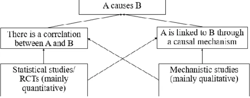
Figure 6. RWT requires the collection of evidence supporting both the claim “there is a correlation between the cause and the effect”, and the claim “there is a mechanism linking the cause and the effect” ... 54

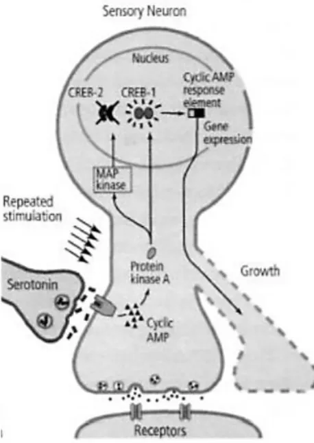
Figure 7. The complex molecular system of long-term facilitation composed of entities (neurons, proteins and genes) and activities (like protein movements and gene expressions) (E. R. Kandel, 2006, p. 204) ... 55

Figure 8. The causal process leading to social revolutions studied by Skocpol (1979) .. 58

Figure 9. The complex social system of segregation. Figure from Cortez and Rica (2015, p. 64) ... 59

Figure 10. The relationship according to which watching violent TV programs increases violent behaviours is masked by another causal mechanism whereby watching violent TV programs decreases violent behaviours. ... 62

Figure 11. The social facilitation mechanism ... 107

Figure 12. The normative influence mechanism ... 108

Figure 13. The network externalities mechanism ... 108

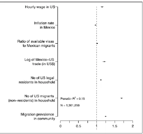
Figure 14. The odds ratio estimates ... 110

Figure 15. The normative influence mechanism can both cause migrants to leave to the U.S., and reinforce the migration culture necessary for this mechanism ... 113

Figure 16. From general to singular causation ... 116

Figure 17. From singular to general causation ... 118

Figure 18. Possible DAGs showing the position of biomarkers ... 131

Figure 19: A mass spectrometry datum for an individual (Fushiki, Fujisawa, & Eguchi, 2006, p. 359) ... 136

(10)

9 Figure 20. The assumption behind process tracing is that the causal path from C to E is mediated through certain factors such as M1, M2 and M3 ... 143

Figure 21. Possible relationships between the surrogate biomarker and the process causing the clinical outcome ... 146 Figure 22. The representation of a constitutive mechanism ... 154 Figure 23. The ideal* intervention I can be a common cause of A and A* because they are related by a non-causal dependency relation... 159 Figure 24. In ideal* interventions, the relationship between A and its acting component A* appears both constitutive and causal ... 160 Figure 25. Possible scenarios with the redundancy-free requirements ... 163 Figure 26. The unbreakability condition ... 164 Figure 27. Spatial entity-involving occurrents and temporal entity-involving occurrents.. ... 169 Figure 28. The general case described by Krickel ... 171 Figure 29. A temporal entity-involving occurrent of S’s Ψ-ing at t1 is the cause of X’s

Φ-ing at t1 ... 173

Figure 30. A temporal entity-involving occurrent of S’s Ψ-ing at t2 is the effect of X’s

Φ-ing at t2 ... 173

Figure 31. The temporal entity-involving occurrents at t1, t2, and t3 are all constituted by

spatial entity-involving occurrents sharing the same temporal regions ... 174 Figure 32. A case of multiple realization ... 179 Figure 33. An extended horizontal surgicality account ... 182 Figure 34. Someone might claim that ACEs are not, like biomarkers (B), signals of the process from socio-economic conditions (SEC) to health outcomes (HO), as shown in (a). ACEs are the causes of the process that, passing through biomarkers (B), could lead to health outcomes (HO). In a similar situation, socio-economic conditions (SEC) might only be correlated to ACEs, without being their cause, like in (b) ... 206

(11)

10

List of Tables

Table 1. Survival rates in the control and treatment groups ... 31

Table 2. Survival rates in the male population ... 32

Table 3. Survival rates in the female population... 32

Table 4. Acceptance rates to the University of California Berkeley in 1973. ... 33

Table 5. Acceptance rates per department to the University of California Berkeley in 1973. ... 33

Table 6. The ten occupation categories of the European Socio-economic Classification (ESeC), retrieved from Rose and Harrison (2007, p. 464)... 127

Table 7. A recap of the terms used in the literature, where they apply and their purpose ... 196

(12)

11

Glossary

Constitutive mechanisms: mechanisms that can explain the phenomena by describing the organizations of entities and activities that actualise the capacity making the phenomena-to-be-explained possible (p. 146)

Etiological mechanisms: mechanisms that, through time, lead to the production of the phenomena-to-be-explained (p. 146)

Mixed methods research (MMR): the combination of quantitative and qualitative methods in the same study (p. 77)

Process tracing: approach to trace the causal chain connecting the putative cause and the putative effect (p. 140)

Russo-Williamson Thesis (RWT): both the identification of a correlation, or difference-making relationship, between the cause and the effect, and the identification of a mechanism linking the cause and the effect are required in order to establish causation (p. 49)

Thick data: in general described as ethnographic, qualitative data collected by researchers (not in automated way) and characterised by contextual complexity which help to recognise not only what people do, but also the reasons behind their activities (p. 42)

(13)

12

1 Introduction

1.1 The emergence of big data

In this thesis, I aim to explore how big data have changed the way in which causal studies are conducted in the social sciences. Over the last few years, the term ‘big data’ has become pervasive, although in several discussions it is not clear what the difference between data and big data is. A careful analysis of the literature, indeed, shows that big data can be defined in different ways, depending on which aspect is highlighted (Kitchin & McArdle, 2016; Schutt & O’Neil, 2013, p. 24).

One of the most popular claims on big data is that such data possess a cluster of characteristics that makes them different from traditional data. Among these features, the most important are claimed to be the so-called ‘Three V’s’: volume, velocity and variety (Laney, 2001). The first ‘V’, volume, can be interpreted in different ways: it might denote the amount of data produced, the size of each datum, or the total storage required by a dataset1. Velocity, furthermore, is considered another vital aspect of big data. With this term, researchers usually indicate the speed at which data are created and at which they can flow from one dataset to another. Finally, the third ‘V’, variety, stands for the numerous formats in which data can be collected. In the social sciences, for instance, relevant data might include structured data such as GPS coordinates and numerical indicators, and unstructured data like satellite images and videos2.

After Laney’s proposal, four additional ‘Vs’ have been proposed in the literature to denote some characteristics or challenges of big data (Khan et al., 2014): validity, veracity, volatility and value. Validity is referred to the correct use of such data, while veracity concerns the truthfulness of data, that may contain bias and inaccuracies, or might be very noisy. Volatility denotes the extent to which data can remain available and reusable over time. Finally, value regards the type of value that can be attributed to data: obviously, data have value because they might provide scientific evidence, but it might also be argued that nowadays data have economic and ethical value. Data and the insights

1_{In all these cases, what should count as a ‘large volume’ remains ambiguous, given that it depends on the}

ability to generate, store and disseminate data. What was considered a ‘large volume’ of data some decades ago, indeed, may not be defined as such nowadays.

2_{Data collected through qualitative studies are in general not included in the definition of big data. As I}

will examine in chapter 2, section 2.4, in the social sciences data collected through qualitative methods are in general considered ‘thick data’.

(18)

17 obtained from them can indeed be traded in the marketplace and can contain personal information on human subjects (for more on this discussion see Borgman, 2016; Kitchin, 2014a; Mayer-Schönberger & Cukier, 2013).

As argued by Kitchin and McArdle (2016), the features represented by such ‘Vs’ cannot be identified in all the datasets that are generally thought to contain big data. The analysis of existing big datasets, in fact, leads to the conclusion that it is impossible to find a cluster of features shared by all big data.

Some examples can help to clarify this observation. First, datasets containing sound sensor data, in general considered big data, consist of amounts of data that are often smaller than the amounts contained in traditional census datasets. In this case, the amounts of data produced are not bigger than the amounts of traditional data. Second, in some cases (like for call records data and GPS data), the size of a big datum is similar, if not smaller, than the size of a traditional datum. Third, in numerous cases big data contained in datasets are not characterised by variety. Datasets containing data generated by sensor devices or financial data, for instance, generally contain only numeric, structured data. Overall, the ‘Vs approach’ provides a broad list of characteristics of big data from which researchers can benefit, and some key challenges that are now at the heart of several methodological and ethical discussions.

In this thesis, I shall adopt the notion of big data I recently developed (Ghiara, 2016, p. 32), according to which big data are in general produced through automated processes and, for this reason, can be created very frequently and almost in real time, as described by the “V” standing for velocity.

My consideration can be combined with the observation that big data have significantly changed scientific practice. As proposed by Leonelli (2014b), the novelty of big data does not reside just in some features that big data have, but in two key changes that have characterised scientific research in the last two decades. The first change concerns the status attributed to data: data are now considered the outputs of scientific research rather than mere side products. To give some examples, new infrastructures such as Figshare and new funded projects such as Understanding Society (https://www.understandingsociety.ac.uk) have been developed with the explicit intention to disseminate data as research outputs in their own. The second change consists

(19)

18 in the development of approaches, infrastructures and skills to format, circulate, retrieve, use and interpret data.

1.2 Big data and causal reasoning

My thesis is focused on how big data are used and interpreted in studies aimed at explaining causal phenomena in the social sciences. This topic has recently been at the heart of several discussions in both the social sciences and philosophy of science. On the one hand, social scientists are wondering how to use the available data to explore causal phenomena and what challenges are associated with big data studies, on the other hand many philosophers of science are studying the links between big data and concepts such as causality and explanation. Questions on the use of big data in causal studies, hence, seem to offer fertile ground to develop scientifically-informed philosophical discussions that can, at the same time, both improve philosophical reflections and clarify scientific practices.

The thesis combines philosophical discussions with scientific arguments and case studies. The starting point is the argument, supported both by philosophers and social scientists, that big data do not offer magical solutions to the challenges that characterise causal studies. Data-driven studies are based on inferential (and often automated) forms of reasoning: they use large amounts of data to create models from them. Yet, data-driven results face the same problems that have already been recognised before the emergence of big data. Some social scientists, furthermore, have added that often data-driven studies do not give due importance to qualitative, ethnographic data, although in the social sciences qualitative approaches have produced valuable insights when used to study causal relationships.

These considerations will be analysed in detail in chapter 2, and will lead me to identify three key challenges of big data for causal studies in the social sciences: i) how to overcome the limitations of data-driven causal studies, ii) how to understand the role of qualitative, ethnographic data in causal studies based on big data, iii) how to use big data, in the social sciences, to obtain evidence of causality that goes beyond correlations. Together with chapter 2, chapters 3 and 4 constitute the first part of the thesis, and examine the first two challenges from a theoretical perspective, drawing some conclusion from conceptual discussions that can be found in the philosophical and social sciences’

(20)

19 literature. More specifically, chapter 3 discusses a way to overcome the limitations of data-driven causal studies, while chapter 4 clarifies how qualitative ethnographic data can improve causal studies based on big data.

Chapter 5 and 6 constitute the second part of the thesis and provide a detailed analysis of two case studies. The case studies are used both to argue in favour of the claims discussed in Part I and to prepare the ground for the proposal that will be discussed in chapter 8 of Part III.

Finally, chapter 7 and 8 compose the third part of the thesis. Such chapters are both focused on how big data can be used, in the social sciences, to obtain evidence of causality that goes beyond correlations. Chapter 7 explores the existing literature on constitutive mechanisms to discuss how constitutive mechanisms are conceptualised and how big data might help to study them. Chapter 8 starts by observing how data have been used in scientific research to trace etiological mechanisms, and then provides a new approach to collect evidence of etiological mechanisms through sociomarkers, the social version of biomarkers.

Overall, the thesis offers three main take-home messages: first, regardless of how sophisticated they are, causal data-driven methods can suffer from bias and their results are in general insufficient to establish causation. To properly establish causation, it is necessary to use both evidence of a correlation between the cause and the effect, and evidence of the mechanism responsible for such a correlation.

Second, the need for mechanistic evidence sheds light on one possible use of qualitative ethnographic data, that can be analysed to collect this type of evidence. Furthermore, qualitative ethnographic data, also called thick data, might be used to study different ontological categories such as those associated with local and general causation, and to study social phenomena from different epistemological perspectives. The importance of such data, therefore, should not be underestimated even in the era of big data.

Third, studying big data does not necessarily mean finding mere correlations between the cause and the effect. Big data can be used to shed light on causal mechanisms, as I argue analysing the use of biomarkers. In the social sciences, the notion of sociomarkers might help researchers to understand how measures obtained from big data can be employed to trace etiological mechanisms. In rare circumstances, furthermore, big data might help to obtain evidence of constitutive mechanisms.

(21)

20

1.3 Methods

My thesis is empirically grounded on the study of existing scientific projects such as Wood’s study on the reasons why peasants in El Salvador decided to join rebel movements (2003) (in chapter 4), Garip and Asad’s study concerning the phenomenon of Mexico–U.S. migration (2016) (in chapter 5), and in the analyses conducted within the project LIFEPATH’s about how socio-economic conditions influence health (in chapter 6). The decision to use real-life scientific examples is consistent with the branch of philosophy of science known by the name of the ‘Philosophy-of-science in practice’, defined as:

“philosophy directly engaged with scientific research through interaction with scientists about philosophical problems” (Boumans & Leonelli, 2013, p. 259)

Since the aim of my thesis is to investigate real scientific challenges associated with big data, one of the first methodological considerations I had to address concerned the best strategy to select research projects. As Boumans and Leonelli argued, one of the pivotal aspects of the Philosophy-of-science in practice is the interaction with scientists: this idea led me to focus on two aspects that helped me to identify what I argue are good case studies. First, I considered whether the researchers involved in such projects were engaged in conceptual and methodological discussions. Second, I considered whether it was possible to receive feedback on my arguments from researchers involved in those or similar scientific projects.

The former aspect (whether the researchers involved in such projects were engaged in conceptual and methodological discussions) helped me to select, among a list of putative case studies, those in which particular attention was spent on epistemological and conceptual questions.

As for the latter aspect, in one case (the case study explored in detail in chapter 6), I managed to directly interact with the researchers involved in the project. Such interactions were informal discussions about the aim of their project and the methodological and conceptual challenges associated with it, and formal presentations during joint workshops (such as the Causality Workshop at Imperial College London), which allowed me to present my research findings and to get feedback on my interpretations.

(22)

21 In the other cases, I managed to obtain feedback from researchers working in the same fields by publishing my material in scientific journals. The material presented in chapters 4 and 5 was published in one article in the Journal of Mixed Methods Research. During the reviewing process I received extensive comments from 3 anonymous reviewers and 2 editors who conduct mixed-methods studies. The material presented in chapter 8, moreover, has been published in Longitudinal and Life Course Studies, and is the result of an interesting discussions with different researchers working both in epidemiology and in the social sciences.

In general, the Philosophy-of-science in practice approach runs the risk of being contaminated with the problem of cherry-picked case studies. Selected case studies might be unrepresentative for different reasons (for instance, only those researchers more interested in conceptual questions might be interested in interacting with philosophers), and this might lead to inferential mistakes if the case studies are taken to be the illustrative cases of general scientific practices.

Although it is extremely difficult (if not impossible) to completely rule out this problem, in my thesis I try to reduce the risk of cherry-picking in two ways. First, I selected different case studies from diverse disciplines in the social sciences. The quantity and variety of cases chosen help me to argue with more conviction that the claims proposed in this thesis can be applied to a broad range of research practices. Second, the claims proposed in the thesis are not proposed as descriptive claims that are applicable to all the possible scientific studies based on big data. Rather, they are proposed as possible (but not unique) ways to overcome some challenges of big data and are claimed to be based on careful considerations based on interesting case studies.

(23)

22

Part I

Methodological debates in the social sciences and

philosophy

The emergence of big data has become a central theme in scientific and philosophical discussions. Both inside and outside academia, there has been growing interest in the potential of big data, as illustrated by the recent surge of dedicated funding, policies and journals. The main tenor of the discussion, shared by academics and non-academics, is that big data allow researchers to think and to do science in a new way.

This idea has been sometimes intensified in the claim that, in the era of big data new statistical methods, rather than existing theories or new approaches to theorising, will drive the practice of science (Anderson, 2008; Mayer-Schönberger & Cukier, 2013). According to these authors, the massive amounts of data now available and the sophisticated algorithms that can be used for data analysis allow scientists to do something unprecedented: to use data for discoveries without taking into account any theoretical element about causation. Causal theories are claimed to be redundant for two reasons: first, sound explanations can be developed just examining the abundant correlations that can be found between data, consequently causal theories are no longer a guide for scientific research; second, big data are making scientists move away from aspiring to understand the reasons why something is happening. In the era of big data, scientists just aspire to understand what is happening:

“Causality won’t be discarded, but it is being knocked off its pedestal as the primary fountain of meaning. Big data turbocharges non-causal analyses, often replacing causal investigations” (Mayer-Schönberger & Cukier, 2013, p. 68)

However influential and exciting, the idea that a data-driven science does not need causal theories and causal investigations has been criticised by scientists and philosophers (Canali, 2016; Floridi, 2012; Kitchin, 2014a; Leonelli, 2014b; Titiunik, 2015), who have cast light on the limitations of big data and on the importance of causal reasoning.

(24)

23 Although these considerations have paved the way for a crucial debate on the use and novelty of big data, more work needs to be done to completely address the questions about big data. In particular, how to use big data in causal studies is still a matter of debate. The overall aim of my thesis is to offer a new answer to this question by examining how big data can be used for causal studies in the social sciences. Part I of the thesis, made of the next three chapters, will provide some clarifications about what problems and solutions have been discussed for causal discoveries in the social sciences and in the philosophy of the social sciences.

Chapter 2 will start by illustrating one of the statistical methods used with big data for causal analysis, Bayesian Networks. This method will be described in detail to show one common way in which data are analysed quantitatively. Next, some of the problems that characterise data-driven studies will be described and applied to Bayesian Networks to clarify how such issues can emerge in real-life data-driven studies. To this, some considerations about the limitations of big data specifically in the social sciences will be added, and the notion of ‘thick’ data will be introduced. Overall, these discussions will lead to the identification of three key challenges of big data for causal studies in the social sciences: i) how to overcome the limitations of data-driven causal studies, ii) how to understand the role of qualitative, ethnographic data in causal studies based on big data, iii) how to use big data, in the social sciences, to obtain evidence of causality that goes beyond correlations. These challenges will be discussed in detail in section 2.5.

Chapter 3 will provide a solution to the first challenge. It will be argued that evidential pluralism, in the formulation proposed by Russo and Williamson (2007), and now known by the name of the Russo-Williamson thesis, can offer a solution to the problems associated with causal data-driven studies in the social sciences. In order to comply with such a thesis, social scientists need to establish both a correlation between the putative cause and the putative effect, and a causal mechanism linking the cause and the effect and producing the statistical relationship between them. While some philosophers of the social sciences have shown scepticism about the usefulness of the Russo-Williamson thesis, I shall argue that it is not only useful, but also in line with how social scientists establish causation.

Chapter 4 will tackle the second challenge by exploring the advantages of combining big and thick data in causal studies. I shall claim that, since thick data are in general defined

(25)

24 as qualitative data, the advantages of such a combination can be explored through the analysis of mixed methods research, based on the combination of quantitative and qualitative approaches. To begin with, I will show that, in mixed methods research, the aim is often to establish the presence both of a correlation and of a causal mechanism between the putative cause and effect, and that this is in accordance with the Russo-Williamson thesis. In these terms, the use of qualitative data is in general justified by claiming that they allow for the identification of causal mechanisms. Next, I shall argue that qualitative data are also used to problematise quantitative findings: the combination of different types of data is used to mix different ontological categories and different epistemological assumptions. In this way, researchers can obtain a comprehensive understanding of the phenomenon under study. Thick data, I shall conclude, can hence be used both to collect evidence of social mechanisms, and to help researchers obtain a comprehensive understanding of the phenomenon under study.

Overall, the following three chapters will help to clarify how the methodological discussions within the social sciences and philosophy of the social sciences communities can be associated with the challenges brought about by big data.

(26)

25

2 No magical solutions with big data

2.1 Introduction

Uncovering causal relationships is vital in many aspects of our daily life: we want to know what affects our health, what might exert an effect on a particular political system, what causes economic crises and so forth. It follows that causal discovery is a problem of interest in almost all the scientific disciplines. Over the last few years this interest has been associated with the discussions regarding the emergence of ‘big data’ and the possibility of automated forms of reasoning. From the beginning of this century, indeed, researchers inside and outside academia have experienced what has been called a ‘data-deluge’. Everywhere we look, it is clear that the quantity of information available is soaring: to give an example, according to some IBM analysts and to the researchers at the International Data Corporation, the total amount of data in the world is now doubled every two years (Giczi & Szőke, 2018; Guo, 2017).

Researchers from different disciplines have tried to find out the best ways to take advantage of this data deluge. Many have argued that new sophisticated data techniques can be used to infer patterns and regularities in the data (Jensen & Nielsen, 2007; Mazzocchi, 2015; Spirtes et al., 2000). Some philosophers, however, have shown that, in real-life scientific practice, there is no such a thing as a purely direct inductive approach (Leonelli, 2014b; Pietsch, 2016). Inferential reasoning from big data, it has been claimed, always requires some theoretical commitments concerning the phenomenon under investigation and the ways in which data are modelled. Many researchers, furthermore, have identified some problems that big data studies might be unable to tackle (see for instance Cartwright, 2007; Floridi, 2012; Hitchcock & Sober, 2004; Kitchin, 2014; Leonelli, 2014b; Raghupathi & Raghupathi, 2014; Titiunik, 2015).

This debate does not represent a sharp division between those who affirm and those who reject the value of inferring patterns from big data. There is a general agreement, indeed, that new statistical methods can make a contribution to the analysis of data. What is seen with scepticism, instead, is the optimism of those who would like to pursue automated forms of scientific reasoning, where the roles played by human activities would be progressively reduced and algorithms would analyse data “better and faster than humans” (Jensen & Nielsen, 2007, p. 24). This position has often been identified with the

(27)

26 expression ‘data-driven science’, according to which inductive and automated forms of reasoning from data should be recognised as a crucial form of scientific inference (Leonelli, 2012a). The scepticism, moreover, is particularly strong when researchers discuss the use of big data for causal studies (Canali, 2016; Clark & Golder, 2015; Kitchin, 2014a; Leonelli, 2014a; Taylor et al., 2008; Titiunik, 2015; Triantafillou et al., 2017). The reason motivating such a reaction is that even though statistical algorithms are becoming more and more sophisticated, there are some difficulties that still today might cause relevant bias in data-driven causal discoveries. The aim of this chapter is to explore such difficulties.

The chapter is structured as follows: in section 2.2 I shall describe Bayesian Networks as an example of machine learning algorithms used to quantitively analyse data. I shall explain why Bayesian Networks can be considered an important statistical approach in the era of big data, and I will show how Bayesian Networks work and the assumptions built into such an approach. In section 2.3 I shall discuss some of the main problems that might threaten the correctness of machine learning’s analyses and for which the solution is not always obvious. More specifically, I will show how machine learning algorithms, in particular circumstances, can generate results that suffer from the so-called Simpson’s paradox, how the high dimensionality of data can have an impact on the capacity to build causal models, and how the quality of data and meta-data remains a challenge even with the most sophisticated algorithms. While such problems are not specific to Bayesian Networks, I shall discuss their impact on Bayesian Networks’ analyses to clarify how they can lead to biased results in real-life situations. Section 2.4 will describe another problem related to big data studies, namely the gap between big, often quantitative, data, and contextual ethnographic data and will show how social scientists are expressing their worries about the limited importance given to the latter type of data. In section 2.5, then, three different challenges of big data will be discussed: i) how to overcome the limitations of data-driven causal studies, ii) how to understand the role of qualitative, ethnographic data in causal studies based on big data, iii) how to use big data, in the social sciences, to obtain evidence of causality that goes beyond correlations. Section 2.6 will conclude the chapter by arguing that new philosophical investigations can help to overcome such challenges.

Overall, the discussion of this chapter will provide some evidence in support of the idea that there are no ‘magical solutions’ with big data: machine learning algorithms can

(28)

27 enhance scientists’ capacity both to extract insights from data and to obtain information concerning specific causal relationships, but bias as well as lack of contextual knowledge might still threaten data-driven results. This observation will pave the way for further philosophical investigations to tackle the challenges proposed at the end of the chapter.

2.2 Bayesian Networks

In the last thirty years several techniques have been proposed to infer causal relationships from observational data, and a new interdisciplinary field, named “causal modelling”, has become particularly important in the study of causal inference. The end of the twentieth century, indeed, was characterised by an explosion of works on this topic, and several important contributions emerged both from fields such as statistics, philosophy and computer science, and from more subject-specific areas like epidemiology and econometrics (for more information see Hitchcock, 2009).

Several sophisticated statistical approaches have been developed to analyse causal relationships in large datasets. Just to mention some of them, data are now analysed through the Principal Component Analysis, Diffusion Maps, Regression Analysis, the Granger Causality Approach, the Structural Equation Modelling and Bayesian Networks. In particular, the set of approaches known by the name of Bayesian Networks (BNs), given its capacity to handle uncertainty in complex domains3_{(Constantinou & Fenton,}

2018) and the possibility of combining BNs with prior knowledge (Heckerman et al., 1995), has become a popular approach in big data studies. New big data projects based on BNs strategies have been funded both in Europe and the U.S. (see for instance the project European funded project BAYES_KNOWLEDGE and the American project Learning Big Bayesian Networks), and many researchers have explored the applications of BNs machine learning algorithms to big data (see for instance Gogoshin et al., 2017; Tang et al., 2016; Wang et al., 2014).

BNs were first developed in the 1980s, but gained popularity from the 1990s and continued to flourish to the present day thanks to some interdisciplinary discussions involving statisticians, computer scientists and philosophers (Korb & Nicholson, 2004; Neapolitan, 2004; Pearl, 1998, 2000; Spirtes et al., 2000; Williamson, 2005, 2010). A

3_{In BNs the uncertainty concerning the model is represented by a probability distribution over the possible}

(29)

28 regular Bayesian Network consists of three components: a finite set V = {V1, ..., Vn} of variables, a directed acyclic graph representing the probability distribution of each variable ∈ V conditional on its parents, and the Markov Condition.

A directed acyclic graph (DAG) consists of a set V = {V1, ..., Vn} of variables, that are used as nodes, and directed edges connecting some pairs of nodes, often called arrows. The graph is acyclic because there are no directed cycles standing for mutual relationships (for instance A → B, B → A), like the one represented in Figure 1.

Figure 1. A directed acyclic graph (DAG).

In BNs, researchers often make free use of the terminology of kinship to denote the different relationships between the vertices. In Figure 1, for instance, C has two parents (A and B, which are its direct causes), while D has 3 ancestors (A, B, C) and no children (therefore no descendants).

The graph is linked to the probability distribution of each variable ∈ V conditional on its parents by means of the so-called Markov Condition, according to which any variable ∈ V is probabilistically independent of all other variables apart from its descendants, conditional on its parents.

Often, graphs in BNs are given a causal interpretation and are called causal graphs. The key assumption behind this causal interpretation associates causal graphs with probability distributions and is formalised in the so-called Causal Markov Condition:

Causal Markov Condition: Each variable is probabilistically independent of its non-effects, given its direct causes

The Causal Markov Condition is part of the definition of causal BNs, and claims that, if we know the value of the direct causes, we should not consider the indirect causes. For instance, in Figure 1, D only depends on C, and it is causally independent of A and B once we conditionalise on its parent C by holding its value fixed. This condition must

(30)

29 always hold if the causal net is to be a BN model: if the Causal Markov Condition is not satisfied, the formalism cannot be interpreted as a Causal Bayesian Network.

The Causal Markov Condition specifies how to obtain probabilistic independencies between variables. However, inferring causation from statistical data in a correct way requires also some knowledge about dependence relationships between variables. This is why, in causal BNs, researchers have proposed the Faithfulness Condition:

Faithfulness Condition: All the probabilistic dependencies and independencies among V are derivable from the causal graph through the Causal Markov Condition

According to the Faithfulness Condition, all probabilistic dependencies and independencies characterising the set of variables under study should be represented in the DAG, otherwise the distribution would be unfaithful to the DAG.

It is important to specify that such a condition, unlike the Causal Markov Condition, does not have to necessarily hold in BNs: even if the Faithfulness Condition is not satisfied, the causal net can still be considered a Bayesian net. If the Faithfulness Condition is satisfied, however, researchers know that the dataset under study has exactly and only the probabilistic independencies shown in the DAG. In other words, the use of this condition has an important inferential advantage: through it, it is possible to say that the model generated from the data implies exactly the dependence and independence relations that are characterising the dataset under study. When the Faithfulness Condition is not satisfied, on the other hand, we cannot be sure that the model obtained represents all and only the dependencies that really characterise the set of variables. The consequence is that, if the Faithfulness Condition does not hold, we might be more likely to draw wrong conclusions about the causal relationships in our dataset.

In the BNs literature, a stock example where the Faithfulness Condition is not satisfied is the DAG representing the relationships between the use of contraceptive pills, thrombosis and pregnancy (Hesslow, 1976, p. 291). On the one hand, contraceptive pills lower the chances of pregnancy; on the other hand, both contraceptive pills and pregnancy increase the probability of thrombosis, as illustrated in Figure 2.

In this case, we have two paths. The first one goes from contraceptive pills to the reduction of the possibility of pregnancy and, hence, the reduction of the risk of

(31)

30 thrombosis (pills →- _pregnancy_→+ _{thrombosis). The second one goes from contraceptive}

pills to the risk of thrombosis (pills →+ _thrombosis).

Figure 2. A directed acyclic graph (DAG) showing the causal relationships between contraceptive pill, pregnancy and thrombosis.

Let us suppose that these two paths are perfectly balanced: the presence of the first path might hide the operation of the second path, and vice versa. The two paths would cancel each other, with the consequence that any probabilistic dependence between contraceptive pills and thrombosis would vanish (i.e. there would not be a probabilistic dependence between pills and thrombosis). Yet, since the DAG shows a path, the probabilistic distribution would be unfaithful to the DAG.

In the statistical and philosophical literature, this and similar problems have been discussed in relation to data-driven methods such as BNs. Originally, BNs were conceived of as belief networks, and the probabilistic relationships were assumed to represent the appropriate degrees of belief for an agent given the data (Pearl, 1988). When BNs are used for machine learning algorithms, however, the probabilistic relationships are in general simply induced by the frequencies observed in the dataset. The DAGs used to infer causal relationships, consequently, are the result of data-driven analyses. In what follows, I shall discuss some of the general limitations that can undermine the usefulness of data-driven studies. Furthermore, to illustrate how these limitations can pose a threat to causal models in specific cases, I shall illustrate the ways in which they can cause bias in BNs.

2.3 Problems with causal modelling

2.3.1 Simpson’s paradox

Suppose you are a doctor reading a paper on a promising new treatment that seems to be very effective. You are excited by the discovery, and you look up the data from the trials to learn more about that. You look at the data concerning male patients and find out that

(32)

31 actually there is no correlation between treatment and recovery. “Well”, you will probably think, “this drug must work very well for female patients”. Then you look at the data about women, and you discover that, also in this case, the treatment does not seem to be effective. How is this possible? How can a drug be bad both for male and female patients, but at the same time good for people? It is clearly problematic if two different analyses induce you to take two opposite actions (give or not the treatment) based on the same data.

This problem is known by the name of ‘Simpson’s paradox’ and was discovered by the statistician Edward Simpson (1951), from whom it took its name. It is based on a statistical phenomenon according to which, in some datasets, subgroups with a common trend (for instance a negative trend) show the reverse trend (a positive trend) when they are aggregated. To illustrate this paradox, let us consider the example proposed by Meek and Glymour (1994, p. 1012). Suppose the data were collected from a study involving 990 patients who divided themselves into a control group (610 patients) and a treatment group (380 patients). Table 1 shows the number of recoveries in the two groups:

Control Group Treatment Group

Alive 260 240

Dead 350 140

Table 1. Survival rates in the control and treatment groups.

By comparing the data about the control group and the treatment group in Table 1, it is possible to conclude that there is a positive association between treatment and survival. Indeed, while in the control group only 260/610 patients survived (43%), in the treatment group the survival rate was 63%.

Suppose that now we look at the same data by distinguishing between male and female patients, as shown in Table 2 and 3.

Male

(33)

32

Dead 320 80

Table 2. Survival rates in the male population.

Female

Alive 100 200

Dead 30 60

Table 3. Survival rates in the female population.

In Table 2 it is possible to see that there is no correlation between treatment and recovery among males: in the treatment group 40/120 (33,3%) of patients survived, in the control group 160/480 (33,3%) of patients recovered from the disease. The percentage of recovery, hence, was the same both in the treatment group and in the control group. In Table 3, furthermore, it is shown that 200/260 (77%) of female patients who were treated survived, the same percentage that was found in the control group, where 100/130 (77%) of the untreated women recovered. Overall, hence, there was no association between treatment and survival among both male and female patients.

There is an explanation for this paradox: when data about women and men were aggregated, the percentage of recovery was calculated by taking into account the weighted average. In other words, the analysis considered how many patients were in each group. Given that women were more likely to recover and, in that specific situation, a larger proportion of women, if compared to the proportion of men, was treated, the results showed that the survival rate in the treatment group was higher than in the control group. Simpson’s paradox is not a rare problem that can be found only in fictional situations. In 1973, the Associate Dean of the graduate school of the University of California Berkeley, by looking at the admission rate data, hypothesised that there was a sex bias in the admission process. The data were indeed shown in a table like Table 4, and it was clear that the denial rate among women was particularly high if compared to the denial rate among men.

(34)

33 Applicants Admitted Denied

Female 1494 2827

Male 3738 4704

Table 4. Acceptance rates to the University of California Berkeley in 1973.

Some years later, in a famous paper, Bickel, Hammel and O’Connell (1975) explored the dataset, observing in detail the percentages of admission for each department. It was thanks to the data analysis performed department by department, that they were able to claim that there was no bias towards women in the admission process. Indeed, by considering the admission rate per department they generated a table similar to the following:

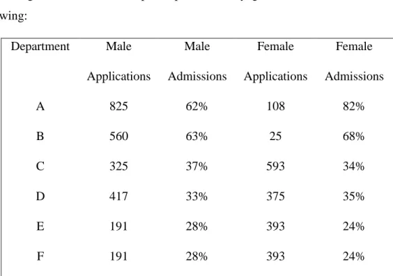
Department Male Male Female Female

Applications Admissions Applications Admissions

A 825 62% 108 82% B 560 63% 25 68% C 325 37% 593 34% D 417 33% 375 35% E 191 28% 393 24% F 191 28% 393 24%

Table 5. Acceptance rates per department to the University of California Berkeley in 1973.

As shown in Table 5, the problem with the admission rate was that female applicants tended to apply more to departments that were more difficult to get into, as the data about department C clearly illustrate. By considering the data properly partitioned, hence, it appears not only that there was not a bias against women, but that there was a small (but statistically significant) bias in favour of women.

(35)

34 While the examples described above are two of the most quoted examples of Simpson’s paradox, it can be noted that several gender bias studies and analyses of sports’ data have provided very nice examples of this phenomenon. For instance, it has been shown that evidence in support of gender bias in science funding is likely to suffer from this paradox (Albers, 2015). From the analysis of basketball’s data, in addition, researchers can claim that a team has the worse shooting in each category, and yet the best overall field goal percentage (Ma & Ma, 2011). In baseball, furthermore, a player A can have a higher batting average for three consecutive seasons if compared to another player B, and yet by combining the three seasons and considering how often each player played, the result is that player B has the higher average (Pearl & Mackenzie, 2018). More examples of this paradox, both in the natural and the social sciences, can also be found in Selvitella’s recent paper entitled ‘The ubiquity of the Simpson’s Paradox’ (2017).

It is now possible to examine how Simpson’s paradox can cause bias in the specific case of BNs. Let us consider again the treatment example discussed above: the treatment apparently worked for the whole population but was ineffective when analysed in the male and female subpopulations. By analysing the overall population divided into a treatment and a control group, researchers would consider just two variables, T (treatment) and R (recovery), and would obtain a causal DAG showing an arrow between T (treatment) and R (recovery), as illustrated in Figure 3(a). This would lead them to give a causal interpretation to the arrow and to establish that the treatment causes recovery. The probabilistic dependence between T and R, however, is actually caused by the common cause G, gender, as illustrated in Figure 3(b). Due to the way in which the control and treatment groups are partitioned, the variable G might not be added in the dataset, with the consequence that the subset of variables analysed might lead scientists to infer a causal relationship that does not exist in reality.

Figure 3. The possible DAGs between treatment, recovery and gender. 3(a) illustrates the probabilistic dependence between T (treatment) and R (recovery), if G (gender) is not considered; 3(b) illustrates the

(36)

35

probabilistic dependencies between G (gender), T (treatment) and R (recovery).

Someone might argue that Simpson’s paradox causes problems especially when researchers analyse small datasets, given that there is a major risk of not considering relevant variables. In big data studies, on the contrary, scientists are able to analyse simultaneously numerous variables, therefore the risk of ignoring important subpopulations could be drastically reduced. This consideration is particularly relevant in specific cases such as medical studies, where it is known that patients’ characteristics such as age and gender can influence physical conditions and recovery, and where such variables are generally available.

In other cases, however, it might be difficult to imagine how to partition data or, in other words, what subpopulations could be relevant to the research question. Human behaviour studies, for instance, in general rely on heterogeneous observational data generated by subpopulations of different sizes. Such behavioural data can now be collected quite easily (for instance, data aboutconsumer behaviours are now collected through the Internet and by platforms such as Amazon, while travel behaviours can be monitored through the use of geolocated data), but at the individual level they often appear very sparse and noisy. It is for this reason that researchers might prefer to aggregate data and to analyse behaviours at the population level. Some examples are the use of population-level data for online activities (such as shopping online) and for diurnal and seasonal mood rhythms (the changes in mood through the day or in different seasons) (Lerman, 2018).

The problem that emerges, however, is that when hundreds or thousands of behavioural data are aggregated, it is not easy to identify the relevant subpopulations. In an online social network, for instance, a large number of variables such as sex, age, occupation, income, education, nationality, average online activities, the number of words per post, and the number of followers might be relevant in order to rule out the possibility of confounders. Some of these factors could be difficult to measure. Furthermore, such variables might be collected in different datasets, and getting access to them could be difficult or very expensive. In a similar situation, what to include or not would finally depend on the researchers’ decisions (with the risk of using inappropriate measures or ignoring important factors). Finally, even when all the possible relevant variables are available and easily measurable, scientists are not immune to inferential errors: too many

(37)

36 variables might indeed cause the curse of dimensionality, which is what I explore in the next section.

2.3.2 High dimensional datasets

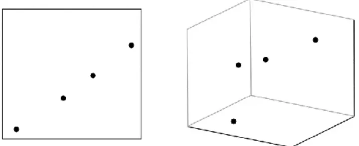
Most of the datasets created in recent years are characterised by high dimensionality, an expression that refers to the situation in which a dataset is characterised by a large number of features. When the number of features is larger than the number of observations, datasets are characterised by the ‘curse of dimensionality’ (Bühlmann & Geer, 2011, p. 1). Suppose we have a dataset containing 100 images (observations) with a high resolution. Each image is composed of thousands or even millions of pixels (in the case of Flickr, for instance, each image can contain 2048x2048 pixels), and each pixel within the image can be understood as a feature of the image. This means that we have a huge number of pixels (features) within each image (observation), and the total number of images is very small if compared to the total number of pixels. The database is hence characterised by high dimensionality. This kind of situation can be found in several contexts: financial datasets, for instance, can contain observations measured daily, hourly, even every minute or second, and for each time slice such datasets have hundreds of features. Similarly, social networks allow for the collection of hundreds of features for each individual using them. Scientific advancements in medicine, finally, have led to the current situation in which thousands of features are collected for each individual, instead of having, as in the past, a big sample with a low dimension (Zeng et al., 2016).

It would be reasonable to hold the intuition that the analysis of high dimensional datasets through machine learning algorithms should offer more accurate results. In reality, however, it is very common that the opposite happens. When datasets are characterised by the curse of dimensionality, as the number of variables increases, the number of plausible combinations of variables explodes exponentially. This happens because a fixed number of data points become increasingly ‘sparse’ if the dimensionality is increased. Figure 4, for instance, represents two cases, one in which we have two dimensions, one in which we have three dimensions: when the dimensionality increases, also the number of sides increases. Consequently, while the data points in two dimensions are sufficient to find a pattern, the same data points in three dimensions are too sparse to enable researchers to select one pattern among all other possible patterns.

(38)

37 Let us consider the case of BNs: as the number of nodes increases, the size of the search space of the relationships between causal nodes grows exponentially in dimensions. If the number of data points, furthermore, is very small if compared to the number of nodes, the confidence in the probability dependences represented in the DAG becomes very low: in other words, we cannot be sure that the complex DAG we are observing represents the correct causal relationships between the nodes under study.

Figure 4. Data points represented in two-dimension space and in three-dimension space.

A phenomenon closely related to the curse of dimensionality is the phenomenon known by the name of ‘overfitting’. When a new algorithm is developed, scientists use training data to train it. Overfitting occurs when the model produced by the algorithm is very accurate on the training data but is much less accurate on the real data. In Figure 5, for example, the curved line best follows the training data if compared to the dashed line, but it might be too dependent on such data. The algorithm producing the curved line, therefore, might have a higher error rate when used with new data. This happens because the set of training data points is too small if compared to the variables analysed, and the algorithm runs the risk of modelling not only the general patterns in the data, but also the idiosyncrasies of that specific data set that are unlikely to recur in further data (Hitchcock & Sober, 2004). This, hence, would cause the model to poorly perform when new data are analysed. For instance, in BNs overfitting typically takes the form of a fully linked DAGs, where the number of arrows is so high that all the nodes of the DAGs are linked to each other.

(39)

38

Figure 5. An example of overfitting (Silipo, 2007, p. 287).

Such considerations bring to the fore what Floridi has called the ‘small pattern’ problem of big data (Floridi, 2012): the vast amount of information available entails that it can be more difficult than in the past to spot where the new relevant patterns lie. Given the growing number of dimensions available for each research question, for instance, how to select the dimensions that can really help both to uncover important patterns and to avoid the curse of dimensionality? To give an example, thousands of genes (features or parameters) are monitored for each person, but for a specific disease only a fraction of them are biologically relevant. It is crucial, hence, to identify those parameters (i.e. dimensions) that can be used for prediction and diagnosis.

In the statistical and computer science literature several methods have been proposed to avoid the curse of dimensionality. One of the most common strategies is to reduce the dimensions of the datasets. Feature transformation techniques, for instance, are data pre-processing methods that allow for the transformation of the original dimensions of a data set into a more compact set of features or parameters, maintaining at the same time as much information as possible (a typical example is Principal Component Analysis). Feature selection algorithms, on the other hand, are based on an alternative approach to dimension reduction and select among the available dimensions the most relevant subset of parameters. Finally, wrapper algorithms use the classification accuracy of some classifier as a criterion to reduce dimensionality (for more details see Cunningham, 2008; Guyon & Elisseeff, 2003).

To avoid some risks associated with the curse of dimensionality and to select the right ‘small patterns’, furthermore, in general researchers work with supervised machine learning algorithms, trained with labelled training datasets containing input objects and the desired output value attached to such objects. To give a simple example, an algorithm can learn to classify animals (such as dogs and cats) after being trained on a dataset containing photos properly labelled with the corresponding species and some identifying features.

There are cases where researchers use unsupervised algorithms, that are thought to be able to recognise processes and patterns without any human guidance. However, in order to improve the reliability of data-driven results, in most of the cases researchers prefer to train the algorithm. In some situations, moreover, scientists’ knowledge is used also to