Comparative Study of MFCC Feature with Different Machine Learning Techniques in Acoustic Scene Classification

ISSN: 2348-7860 (O) | 2348-7852 (P) | Vol. 5 No. 7 | July 2018 | PP.

439-444

Digital Object Identifier DOI

®

http://dx.doi.org/10.21276/ijre.2018.5.7.1

Copyright © 2018 by authors and International Journal of Research and Engineering

This work is licensed under the Creative Commons Attribution International License (CC BY).

creativecommons.org/licenses/by/4.0

|

|

ORIGINAL ARTICLE

Comparative Study of MFCC Feature with Different Machine

Learning Techniques in Acoustic Scene Classification

Author(s): *

1

Mie Mie Oo

Affiliation(s):

1

Faculty of Computer System and Technologies,

University of Computer Studies, Mandalay, Myanmar

*Corresponding Author: [email protected]

Abstract: The task of labelling the audio sample in

outdoor condition or indoor condition is called

Acoustic Scene Classification (ASC). The ASC use

acoustic information to imply about the context of

the recorded environment. Since ASC can only

applied in indoor environment in real world, a new

set of strategies and classification techniques are

required to consider for outdoor environment. In

this paper, we present the comparative study of

different machine learning classifiers with

Mel-Frequency Cepstral Coefficients (MFCC) feature.

We used DCASE Challenge 2016 dataset to show

the properties of machine learning classifiers.

There are several classifiers to address the ASC

task. In this paper, we compare the properties of

different classifiers: K-nearest neighbours (KNN),

Support Vector Machine (SVM), Decision Tree

(ID3) and Linear Discriminant Analysis by using

MFCC

feature.

The

best

of

classification

methodology and feature extraction are essential

for ASC task. In this comparative study, we extract

MFCC feature from acoustic scene audio and then

extracted feature is applied in different classifiers

to know the advantages of classifiers for MFCC

feature. This paper also proposed the

MFCC-moment feature for ASC task by considering the

statistical moment information of MFCC feature.

Keywords: Acoustic scene classification; DCASE 2016; K-nearest neighbors (KNN); Support Vector Machine (SVM); Decision Tree (ID3) and Linear Discriminant Analysis (LDA); MFCC; statistical moment;

I.

INTRODUCTION

Acoustic Scene Classification (ASC) is receiving wide spread attention due to its wide variety of applications in smart Wearable devices, surveillance, life log diarization, context-aware services, etc. The classification of acoustic scenes is an emerging area of research in various studies of machine listening. Increase in interest in this area in recent years, largely due to the Classification of Acoustic Scenes and Events DCASE challenges established in 2013. The DCASE challenges have attracted a large number of submissions designed to solve the problem of acoustic scene classification.

A typical ASC system requires a feature extraction stage in order to reduce the complexity of the data to be classified. The key is the coarsening of the available data such that similar sounds will yield similar features generalization, and the features should be distinguishable from those yielded by different types of sounds discrimination. Generally, the audio is split into frames and some kind of mathematical transform is applied in order to extract a feature vector from each frame. Features extracted from labelled recordings are used to train some form of classification algorithm, which can then be used to return labels for new unlabelled recordings.

To overcome the challenges of ASC, the convolutional neural network based on the architecture of network-in-network is proposed to utilize in building the classifier audio signal. For the feature extraction part, mel frequency spectral coefficients (MFCC) is used as the input vector for the classifier. 1-D convolution operation instead of performing 2-D convolution is used unlike from the original architecture of network-in-network. Every frame from MFCC feature set are used, and the results for every frames are then threshold and voted to choose the final scene label of audio data DCASE challenge for both development and evaluation dataset [1].

Matching Pursuit (MP) algorithm is applied in order to extract Time-Frequency (TF) based features to identify audio features. MP algorithm is used to select atoms iteratively among the set of parameterized waveforms in the dictionary that best correlates the original signal structure. The mean and standard deviation of amplitude and frequency parameters of first few (n) atoms are calculated separately by Using these selected set of atoms, resulting into four MP feature sets. The combination of MFCCs and MP features is proposed to get the best recognition accuracy of GMM classification [2]. The CNN approach is proposed to beat a Gaussian mixture model baseline for the DCASE 2016 database even though training data is sparse [5].

To explore the advantages of the feature extraction and classification methods, the different feature extracting methods: MFCC, LFCC, Anti-MFCC, Chroma and APGD features with different classification algorithms: GMM and Deep Neural Network (DNN) are compared. DNN worked better with different features over the DCASE-2013 [4].

To define a general framework for ASC and present different implementations of its components, the wide ranges of different algorithms are presented for audio data challenge. MFCCS, GMMS and a maximum likelihood are defined as baseline method for framework of ASC to evaluate the algorithms and statistical significance tests to compare the presented methods [3].

Here we investigate the ASC problem using different classification methods to know the advantages of classifiers. The propose ASC system consists of:

1) Extract MFCC feature from audio clips at the scene level

2) Classify extracted MFCC feature with different machine learning classifiers

3) Measure average classification accuracy of different classifiers on 10-fold cross validation

Rest of the paper is listed as follows. Section II presents the general framework of Acoustic Scene Classification. Section III includes MFCC feature extraction and the brief review on various machine learning classification methods in Acoustic Scene Classification. Section IV presents the experimental results on different classifiers. Then section V concludes this paper along with possible future works.

II.

ACOUSTIC

SCENE

CLASSIFICATION

(ASC)

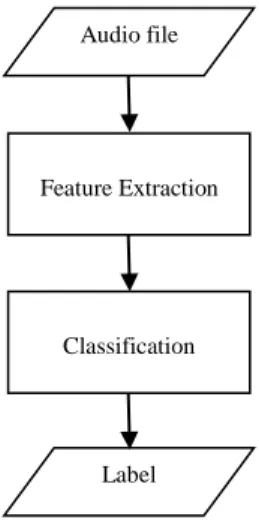
The general workflow of an ASC system is usually divided into two major steps in figure 1.

1) Feature Extraction

2) Classification.

Figure 1: General workflow of an ASC system

 Feature Extraction: a mathematical representation for audio signal data. The MFCC feature is extracted to represent the audio signal data in the form of 32x32 matrixes. The Kth orders of centralized moments are calculated form extracted MFCC feature to extract the statistical feature of MFCC feature (K=2, 3, 4, 5, 6, 7).

 Classification: a classifier to predict the labels unknown audio signal data according to the application domain. The supervise machine learning techniques: K-nearest neighbours (KNN), Support Vector Machine (SVM), Decision Tree (DT) and Linear Discriminant Analysis (LDA) are used to build the classifiers.

III.

FEATURE

EXTRACTION

AND

MACHINE

LEARNING

CLASSIFICATIONS

A. Mel-Frequency Cepstral Coefficients (MFCCs)

Feature

Mel-frequency cepstral coefficients (MFCCs) are coefficients and derived from a type of cepstral representation of the audio clip. MFCCs are commonly derived as follows [8]:

 Take the Fourier Transform of (a windowed excerpt of) a signal.

 Map the powers of the spectrum obtained above onto the mel scale, using triangular overlapping windows.

 Take the logs of the powers at each of the mel frequencies.

 Take the discrete cosine transform of the list of mel log powers, as if it were a signal.

Audio file

Feature Extraction

Classification

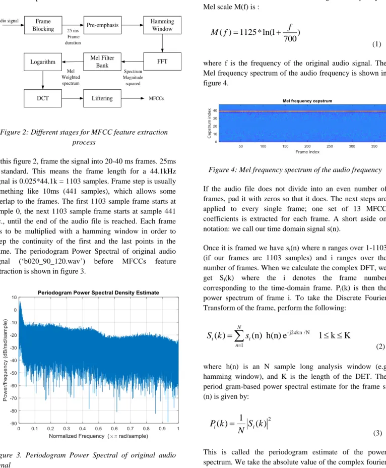
 The MFCCs are the amplitudes of the resulting spectrum. Frame Blocking Pre-emphasis Hamming Window Liftering FFT DCT Logarithm 25 ms Frame duration Spectrum Magnitude squared Mel Weighted spectrum Audio signal Mel Filter Bank MFCCs

Figure 2: Different stages for MFCC feature extraction process

In this figure 2, frame the signal into 20-40 ms frames. 25ms is standard. This means the frame length for a 44.1kHz signal is 0.025*44.1k = 1103 samples. Frame step is usually something like 10ms (441 samples), which allows some overlap to the frames. The first 1103 sample frame starts at sample 0, the next 1103 sample frame starts at sample 441 etc., until the end of the audio file is reached. Each frame has to be multiplied with a hamming window in order to keep the continuity of the first and the last points in the frame. The periodogram Power Spectral of original audio signal (‘b020_90_120.wav’) before MFCCs feature extraction is shown in figure 3.

Figure 3. Periodogram Power Spectral of original audio signal

After Framing Window, the system converts the frequency of original signal into Mel-Frequency by using Mel Filter Bank. The Mel scale relates perceived frequency, or pitch, of a pure tone to its actual measured frequency. Humans are much better at discerning small changes in pitch at low frequencies than they are at high frequencies. Incorporating

this scale makes our features match more closely what humans hear. The formula for converting from frequency to Mel scale M(f) is :

)

700

1

ln(

*

1125

)

(

f

f

M





(1)

where f is the frequency of the original audio signal. The Mel frequency spectrum of the audio frequency is shown in figure 4.

Figure 4: Mel frequency spectrum of the audio frequency

If the audio file does not divide into an even number of frames, pad it with zeros so that it does. The next steps are applied to every single frame; one set of 13 MFCC coefficients is extracted for each frame. A short aside on notation: we call our time domain signal s(n).

Once it is framed we have si(n) where n ranges over 1-1103 (if our frames are 1103 samples) and i ranges over the number of frames. When we calculate the complex DFT, we get Si(k) where the i denotes the frame number corresponding to the time-domain frame. Pi(k) is then the power spectrum of frame i. To take the Discrete Fourier Transform of the frame, perform the following:

K

k

1

e

h(n)

(n)

)

(

-j2 kn / N 1









  N n i i

k

s

S

(2)

where h(n) is an N sample long analysis window (e.g hamming window), and K is the length of the DET. The period gram-based power spectral estimate for the frame si (n) is given by: 2

)

(

1

)

(

S

k

N

k

P

_i



_i (3)

This is called the periodogram estimate of the power spectrum. We take the absolute value of the complex fourier transform, and square the result. We would generally perform a N point FFT and keep only the first C coefficients.

Compute the Mel-spaced filter bank. This is a set of 20-40 (25 is standard) triangular filters that we apply to the periodogram power spectral estimate from step. To calculate filter bank energies we multiply each filter bank with the

power spectrum, then add up the coefficients. Take the log of each of the energies from step 3. This leaves us log filter bank energies. Take the Discrete Cosine Transform (DCT) of the log filter bank energies to give cepstral coefficients [8]. The periodoram power spectral of the extracted MFCC feature for the audio (‘b020_90_120.wav’) is shown in figure 5.

Figure 5: Periodoram power spectral of the extracted MFCC feature of audio signal

B. Centralized Order of Moment

The central moment of order

k

of a distribution is defined as

k

k

E

x

m



(





)

(4) where E(x) is the expected value of x. The central first moment is zero, and the second central moment is the variance computed using a divisor of n rather than n – 1, where n is the length of the vector x or the number of rows in the matrix X.

C. Machine Learning Classification Algorithms

Classification is a supervised data mining technique that assigns labels to a collection of data in order to get more accurate predictions and analysis. The ASC is the task to assigns label to audio data to know the label of audio by using trained classifier. The labels for unknown audio data may different according to the application domain. In this proposed work, K-nearest neighbors (KNN), Support Vector Machine (SVM), Decision Tree (ID3) and Linear Discriminant Analysis are used to make the analysis of very large datasets effective.

D. K-Nearest Neighbors

A powerful classification algorithm used in pattern recognition. KNN stores all available cases and classifies new cases based on a similarity measure [6]. A non-parametric lazy learning algorithm:







N n i

k

k

S

1

yi

1

)

(

(5)

The system calculates distance between new example and all data in the training set. The Euclidean distance between X = [x1,x2,x3,..,xn] and Y = [y1,y2,y3,...,yn] D(X,Y) is defined as:









N n

yi

xi

Y

X

D

1

)

2

)^

((

)

,

(

(6)

E. Support Vector Machines

The Support Vector Machines (SVM) is a supervised learning method for classification and Regression. SVM finds Hyperplane with maximal separation between it and closest data points. There exist a way to compute inner product in feature space as function of original input points. Some commonly used kernel functions are:

Linear: K(X,Y) = XTY (7)

Polynomial of degree d: K(X,Y) = (XTY+1)d (8)

Gaussian Radial Basis Function (RBF): K(X,Y) = e –k (9)

where k = - (||X-Y||)/(22). [7]

F. Decision Tree

Decision Tree (DT) is a tree where the root and each internal node are labeled with a question. The arcs represent each possible answer to the associated question. Each leaf node represents a prediction of a solution to the problem. DT is a popular technique for classification; Leaf node indicates class to which the corresponding tuple belongs. A Decision Tree Model is a computational model consisting of three parts:

1) Decision Tree

2) Algorithm to create the tree

3) Algorithm that applies the tree to data

The DT needs to consider issue in over fitting, rectangular partition and pruning while construction of DT.

G. Linear Discriminant Analysis

Linear discriminant methods group data of the same classes and separates data of the different classes. Linear discriminant analysis finds a linear transformation (discriminant function) of the two predictors, X and Y that yields a new set of transformed values that provides a more accurate discrimination than either predictor alone:

Transformed Target = ( C1 * X ) + ( C2 * Y ) (10) 442

IV.

EXPERIMENTAL

RESULTS

In training, the MFCC features are extracted from all data of DCASE dataset and then train different classifiers for experimental performance. In testing, the MFCC feature is extracted from input audio file and predicts the label using extracted MFCC feature with trained classifier. For theatrical excluded value of validation for classifier, this experiment use 10-Fold cross validation over DCASE dataset with different classifiers.

A. DCASE 2016 Dataset

The DCASE 2016 dataset is a challenges dataset for ASC because it collected sound from different conditions and environments. This research work uses this dataset to overcome location invariant and noise invariant. It consists of 1170 audio files in wav format with 15 labels [11]. Acoustic scenes for 15 labels are:

 Bus - traveling by bus in the city (vehicle)

 Cafe / Restaurant - small cafe/restaurant (indoor)

 Car - driving or traveling as a passenger, in the city (vehicle)

 City center (outdoor)

 Forest path (outdoor)

 Grocery store - medium size grocery store (indoor)

 Home (indoor)

 Lakeside beach (outdoor)

 Library (indoor)

 Metro station (indoor)

 Office - multiple persons, typical work day (indoor)

 Residential area (outdoor)

 Train (traveling, vehicle)

 Tram (traveling, vehicle)

 Urban park (outdoor)

B. 10-Fold Cross Validation

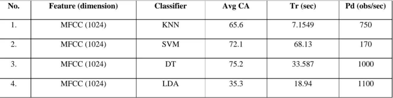
A cross-validation setup is provided for the development dataset in order to make results reported with this dataset uniform. The setup consists of ten folds distributing the 78 available segments based on location. The average classification accuracy (Avg CA), training time (Tr) in sec and prediction speed (Pd) in observations/sec for all classifiers are calculated over 10-folds cross validation are shown in table 1. In table 1, the MFCC feature is extracted from audio file and resized into 32*32 matrix.

Then extracted MFCC feature is classified by using trained classifier. The flow of MFCC feature extraction for this experiment is shown in figure 6.

Figure 6: Flow of MFCC feature extraction

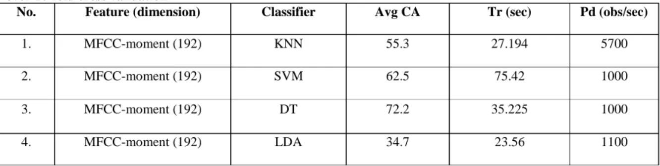
We also perform the next experiment for statistic of MFCC feature with different classifier. In this experiment, the MFCC feature is extracted from audio file and resized into 32*32 matrixes. Then extracted kth order of central moment (k= 2, 3, 4, 5, 6, 7) is calculated from extracted MFCC feature to classify by trained classifier. The flow of MFCC feature extraction for this second experiment is shown in figure 7.

Figure 7: Flow of MFCC-moment feature extraction

Audio file MFCC feature extraction MFCC feature

Table I: Comparison of average classification accuracy for MFCC features with different classifiers over 10-fold cross validation

No. Feature (dimension) Classifier Avg CA Tr (sec) Pd (obs/sec)

1. MFCC (1024) KNN 65.6 7.1549 750 2. MFCC (1024) SVM 72.1 68.13 170 3. MFCC (1024) DT 75.2 33.587 1000 4. MFCC (1024) LDA 35.3 18.94 1100 Audio file MFCC feature extraction MFCC-moment feature Kth _{order of} central moment calculation

In table 1 and table 2, for KNN classifier, the model type used Cosine Distance metric with k (Number of neighbors) is 1. For SVM classifier, the model used quadratic kernel function; automatic kernel scale and box constraint level 1. The model type of the DT used Bagged Trees Preset, Bag Ensemble method and 30 learners to build DT classifier.

V.

CONCLUSION

MFCC feature is one of the good features which have acceptable average classification accuracy with different machine learning classifications. Our comparative study of different classifiers with MFCC feature has reasonable classification accuracy to solve the difficulties in choosing best classifiers for ASC. The moment statistic of MFCC features called MFCC-moment also has acceptable classification accuracy for ASC. For future work, different spectro-temporal representations and different features will be investigated for a set of innovative features for best classification accuracy in ASC. Although both MFCC and MFCC-moment features have acceptable classification accuracies with machine learning classifiers, we need to try to improve the classification accuracy of ASC by considering other signal processing techniques and deep learning classifiers.

VI.

DECLARATION

Author has disclosed no conflicts of interest and the project was self-funded.

REFERENCE

[1] Santoso, A., Wang, C.Y. and Wang, J.C., 2016. Acoustic scene classification using network-in-network based convolutional neural network-in-network. DCASE2016 Challenge, Tech. Rep.

[2] Mulimani, M. and Koolagudi, S.G., 2016. Acoustic scene classification using MFCC and MP features. Tech. Rep.

[3] Barchiesi, D., Giannoulis, D., Stowell, D. and Plumbley, M.D., 2014. Acoustic scene classification. arXiv preprint arXiv:1411.3715.

[4] Patiyal, R. and Rajan, P., 2016. Acoustic scene classification using deep learning. IEEE AASP Challenge on Detection and Classification of Acoustic Scenes and Events (DCASE).

[5] Battaglino, D., Lepauloux, L., Evans, N., Mougins, F. and Biot, F., 2016. Acoustic scene classification using convolutional neural networks. IEEE AASP Challenge on Detec.

[6] Tilani Gunawardena, 2017. Algorithms: K Nearest

Neighbors. URL:

https://www.slideshare.net/heghbalz/slides-of-my-presentation-at-eusipco-2017.

[7] Prakash B. Pimpale , 2013. Support Vector

Machines. URL:

https://www.slideshare.net/pbpimpale/support-vector-machine-24419322.

[8] Prahallad, K., 2011. Speech technology: A practical introduction, topic: Spectrogram, cepstrum and mel-frequency analysis. URl: http://www. speech. cs. cmu. edu/15-492/slides/03_mfcc. pdf.

[9] J. Wilku, 2012. DATA WARE HOUSING AND DATA MINING : Decision Tree. URL: https://www.slideshare.net/jagjitsinghwilku/decisio n-trees-14788315

[10] Suraj Kumar and Saroj Paswan, 2014. FACE RECOGNITION USING FISHER FACE ANALYSIS(LDA) .URL:

https://www.slideshare.net/sk19920909/lda-40913540

Table II: Comparison of average classification accuracy for MFCC-moment feature with different classifiers over 10-fold cross validation

No. Feature (dimension) Classifier Avg CA Tr (sec) Pd (obs/sec)

1. MFCC-moment (192) KNN 55.3 27.194 5700

2. MFCC-moment (192) SVM 62.5 75.42 1000

3. MFCC-moment (192) DT 72.2 35.225 1000