Models for early prediction of at-risk students in a course using standards-based grading

(1)

Models for early prediction of at-risk students in a course

using standards-based grading

Farshid Marbouti

a,*

, Heidi A. Diefes-Dux

b

, Krishna Madhavan

b

a_{San Jose State University, USA} b_{Purdue University, USA}

a r t i c l e i n f o

Article history:

Received 6 October 2015

Received in revised form 9 September 2016 Accepted 14 September 2016

Available online 15 September 2016

Keywords: Learning analytics Predictive modeling Students success First-year engineering Standards-based grading

a b s t r a c t

Using predictive modeling methods, it is possible to identify at-risk students early and inform both the instructors and the students. While some universities have started to use standards-based grading, which has educational advantages over common score-based grading, aterisk prediction models have not been adapted to reap the benefits of standards-based grading in courses that utilize this grading. In this paper, we compare predictive methods to identify at-risk students in a course that used standards-based grading. Only semester performance data that were available to the course in-structors were used in the prediction methods. When identifying at-risk students, it is important to minimize false negative (i.e., type II) error while not increasing false positive (i.e., type I) error significantly. To increase the generalizability of the models and accuracy of the predictions, we used a feature selection method to reduce the number of variables used in each model. The Naive Bayes Classifier model and an Ensemble model using a sequence of models (i.e., Support Vector Machine, K-Nearest Neighbors, and Naive Bayes Classifier) had the best results among the seven tested modeling methods.

1. Introduction

Despite numerous efforts to improve student retention and success in higher education institutions over the past 30 years, retention rates remain low (Gardner&Koch, 2012). According to theNational Collegiate Retention and Persistence to Degree Ratesreport in 2012, theﬁrst to second year retention rate on average was 66.5% (ACT, 2012). Almost one third of students leave college after experiencing just theirﬁrst year. The attrition continues through the next years of school - only 45% of students who enter college graduate after 5 years (ACT, 2012). Academic success is the most important factor in students' retention and the best predictor of students persistence (DesJardins, Ahlburg,&McCall, 1999; Pascarella&Terenzini, 2005). Risk of attrition decreases with an increase in academic achievement (Murtaugh, Burns,_&Schuster, 1999). Thus, one way to increase retention is to increase academic success.

Theﬁrst step to increasing academic success is the identiﬁcation of at-risk students early in the semester. Through the use of predictive modeling techniques, it is possible to forecast students' success in a course and identify those that are at-risk (Jin, Imbrie, Lin,&Chen, 2011; Lackey, Lackey, Grady,&Davis, 2003; Olani, 2009). A predictive model can be used as an early warning system to identify at-risk students in a course and inform both the instructor and the students. Instructors can then

*Corresponding author.

E-mail address:[email protected](F. Marbouti).

Contents lists available atScienceDirect

Computers & Education

j o u r n a l h o m e p a g e : w w w . e l s e v i e r . c o m / l o c a t e / c o m p e d u

http://dx.doi.org/10.1016/j.compedu.2016.09.005

(2)

use a variety of strategies to communicate with the at-risk students and provide them pathways for improving their per-formance in the course. Use of an early warning system in a course, along with intervention guidelines, can increase students’ success in a course (Arnold&Pistilli, 2012; Essa&Ayad, 2012; Macfadyen&Dawson, 2010).

Despite the promise of academic early warning systems (e.g., Course Signals,Pistilli&Arnold, 2010), the existing ones have some shortcomings. First, one common and major problem is that they typically employ a general prediction model that cannot address the complexity of all courses. Employing a general prediction model can result in low accuracy predictions of students' success in a course because the course learning objectives, activities, and assessments can vary a great deal. For instance, being successful in a course that employs active learning strategies can be very different than a course that only employs lecture. Second, most early warning systems have been designed for online courses or rely heavily on Course Management System (CMS) access data (e.g., OU Analyze (Kuzilek, Hlosta, Herrmannova, Zdrahal,&Wolff, 2015)) and not performance data, which may not be a suitable data source for many face-to-face courses because many learning activities happen outside of the CMS. Third, early warning systems do not employ models optimized to identify at-risk students who need accurate predictions the most. Because grades are usually negatively skewed (i.e., the number of students who fail a course is fewer than number of students who pass the course), the models accuracy is higher for the students who pass the course and lower for those who fail. Fourth, all early warning systems have been developed based on summative score-based grading, which is typically norm-referenced. Some universities have started to change their grading from summative score-based to standards-score-based systems, which has educational advantages described below. Thus, academic early warning systems should adapt their models to this new grading system.

Standards-based grading is based on_“the measurement of the quality of students pro_ﬁciency towards achieving well deﬁned course objectives”(Heywood, 2014, p. 1514) and grades“represent how well students achieve the course objectives” (Sadler, 2005, p. 179). Standards-based grading is criterion-referenced not norm-referenced. In other words, students are graded based on their achievements or what they can do, regardless of how other students in the course perform on the same assigned task (Carberry, Siniawski,&Dionisio, 2012; Heywood, 2014; Sadler, 2005). In this grading system, the course as-sessments are directly connected to the course learning objectives and are not a series of separate course assignments (Carberry et al., 2012).

Standards-based grading provides educational advantages for students. Because standard-based grading assesses stu-dents' achievement of the course learning objectives, it provides clear, meaningful, and personalized feedback for students related to achievement of the course learning objectives and helps them identify their weaknesses in the course (Atwood& Siniawski, 2014). In addition, because the students are aware of course learning objectives and a student's grade is inde-pendent of other students' performance, it provides“fairness and transparency”(Sadler, 2005). Because of its educational advantages, it is expected that more universities and courses will employ standards-based grading in the near future and it is important that early warning systems change their models accordingly.

Extensive research has been conducted to determine the factors that correlate to and/or predict students' academic success in a course. The majority of these studies focused on predicting students' grade in a course at the end of the semester using academic factors available before the start of the semester (e.g., cumulative GPA, grade in a pre-requisite course) and non-academic factors (e.g., gender, age). Neither course instructors nor students can inﬂuence past performance indicators (e.g., student GPA, previous grades) or many non-academic factors (e.g., gender, race, socio-economic status). If students are made aware of that these factors are used in the prediction models, it may discourage them because they may think their past behavior or circumstances have set them up for failure and there is nothing they can do to achieve positive future outcomes. Thus these models, despite their intention to help students, may negatively affect students' performance. More research is needed to investigate the positive and negative effects of using and sharing the basis for prediction models for students learning.

A few studies have utilized the academic performance data available during the semester, which logically can be the best predictor of the course grade. One such study compared four different methods to predict students' grades in an engineering Dynamics course using 323 students' data from four semesters (Huang_&Fang, 2012). In this study, three midterm exam grades were used as indicators of students' performance during the semester. In addition, students' cumulative GPA and grades in four pre-requisite and Dynamics-related courses (i.e., Statics, Calculus I and II, and Physics) were used as indicators of students' performance before starting the course. Students' grades at the end of the semester were predicted using four different prediction methods, which in the best case predicted 64% of the students course grades. A comparison of different models revealed that adding grades from pre-requisite courses to GPA does not result in a signiﬁcant increase in the accuracy of the model. Furthermore, using only theﬁrst mid-term exam with an accurate prediction method yields an overall 52.5% accuracy, which is similar to using pre-course performance data such as GPA or previous course grades. These results clearly demonstrate the value of using performance data gathered during the semester for predictive purposes. Adding other per-formance data such as homework and quiz grades could increase the accuracy of the models. Also unlike mid-term exams, homeworks and quizzes start earlier in the semester and using them as predictors of success may result in accurate pre-dictions early in the semester.

In a previous study, we built three logistic regression-based models to identify at-risk students (deﬁned as getting a D or F grade in the course) in a largeﬁrst-year engineering course at three important times in the semester according to the aca-demic calendar: at weeks 2, 4, and 9 (Marbouti, Diefes-Dux,&Strobel, 2015). For the weeks 2 and 4 models, we only used attendance records, homework, and quiz grades. For the week 9 model, mid-term exam grades were also used. The models were optimized for identifying at-risk students and were able to identify at-risk and successful students with overall accuracy

(3)

of 79% at week 2, 90% at week 4, and 98% at week 9. This high prediction accuracy illustrates the value of creating course speciﬁc prediction models instead of generic ones and using performance-based data during the semester.

A number of different prediction methods have been used in educational settings for a variety of purposes. Different methods result in different accuracies in different settings. For example, to predict gradesHuang and Fang (2012)used multiple linear regression (MLR), multilayer perceptron (MLP) neural network, radial basis function (RBF) neural network, and support vector machine (SVM) (see section3.3or (Hand, Mannila,&Smyth, 2001) for more details about these methods). The SVM model had the highest overall accuracy (64%) among the different models. Some of the commonly used prediction methods in data mining, such as Naive Bayes Classiﬁer (NBC) or K-Nearest Neighbors (KNN), hold promise for identifying at-risk students because they are being used in other contexts and provide promising results. So, not only the prediction model variables (e.g., homework and midterm exam grades) but also the prediction modeling methods are important in achieving predictions with desired accuracy. In this paper, we compare some of the common prediction methods toﬁnd the best methods for identifying at-risk students.

2. Research purpose and research questions

It is crucial to identify at-risk students as early as possible during a course. With the shortcomings of current academic early warning systems it is important to develop prediction models with high accuracy for at-risk students. Logically, the academic performance data available during the semester can be the best predictor of the course grade. Using learning objective scores in addition to typical score-based graded assessments may have advantages in prediction models that have not been investigated. In this paper, we compare seven different predictive modeling methods using only academic factors (i.e., learning objective achievement scores and grades during the semester) that are available to the course instructor during the semester. The goal is toﬁnd the best prediction method for identifying at-risk students while showing the accuracy and usability of course-speciﬁc standards-based prediction models by answering the following research questions:

Of six different predictive modeling methods, as well as a seventh hybrid or Ensemble method (consisting of three of the most successful individual methods), which is the most successful at identifying at-risk students, based on spec-iﬁed in-semester student performance data? Why is this method the most successful? Why are the other methods less successful?

3. Methods

3.1. Participants and settings

This study uses secondary data collected during the Spring 2013 and Spring 2014 semester offerings of aﬁrst-year en-gineering (FYE) course at a large Midwestern U.S. university. In Spring 2013 1650 and in Spring 2014 1413 FYE students enrolled in the course. The course was offered in 15 different sections of a maximum of 120 students. Each section had one instructor and six teaching assistants who graded the assignments. This course is a mandatory second semester, 2-credit hour course for all FYE students. In this course, students learn how to use computer tools to solve fundamental engineering problems; how to make evidence-based engineering decisions; develop problem-solving, modeling, and design skills; and develop teaming and communication skills. This course is a good example to showcase how to create and use predictive models for a course because it enrolls a large number of students and it involves several different graded components (e.g., quizzes, homeworks, exams, projects) most of which are collected on a weekly basis. Thus, this course generates a large number of performance data each week.

3.2. Data

The students' performance data (i.e., achievement of learning objectives and course grades book) from Spring 2013 were randomly (with control for pass/fail ratio) divided into three datasets: 50% for training, 25% for comparing different methods and tuning the models, and 25% for the secondary testing after improving the models. Spring 2014 data was used forﬁnal testing of the models. Because in practice the instructors can only build the model based on a previous semester's data (i.e., training dataset) and use it during the current semester to help students (i.e. test data), we simulated this process in our study design in order to verify how the prediction models will actually work if an instructor decide to use them. The in-semester student performance data for this course included grades for attendance, quizzes, and weekly homework as well as team participation, project milestones, mathematical modeling activity tasks, and exams (Table 1). Within a section, all grading was done by the course instructor and teaching assistants.

In this paper, performance data available at the end of week 5 of the semester, which included the homework learning-objectives scores and grades for quizzes and written exam 1, referred to in this paper as midterm exam, were used. Each homework was designed and graded based on 6_e7 learning objectives. For example, the week 3 topic was related to cu-mulative distribution plots. This week's homework had seven learning objectives including 1) Demonstrate the ability to create a histogram for technical presentation using Excel, 2) Construct cumulative distribution plots in Excel, 3) Interpret cumulative distribution plots, 4) Construct and interpret cumulative distribution plots in MATLAB, 5) Construct a _ﬁgure

(4)

window to display multiple plots and/or histograms, 6) Apply coding standards (e.g., by properly commenting and creating suf_ficiently descriptive variable names), and 7) Exhibit professional habits (by properly using the course template, using specified variable names, and submitting all necessaryfiles).Appendix Alists the homework learning objectives for thefirst five weeks of the semester. Learning objectives were assessed on a four level scale: no evidence (0), under achieved (1), partially achieved (2), or fully achieved (3). Rubric guides explicated to the graders what students needed to demonstrate to achieve each level. For instance, for learning objective 2, the grader would assign a level of fully achieved if the student demonstrated that she can generate a cumulative distribution plot using histogram data and the six step approach, proper label the x-axis and y-axis (with units where appropriate), and provide a descriptive title (includes sample or population size). A partially achieved level assignment would be made if one or two of these things were missing. The learning objective and both the level and written feedback are provided to the student via the rubric tool available through the course management system used in this course.

Quizzes and exams were designed based on the learning objectives but graded with a traditional score point system. For example, one of the midterm exam problems was:

Problem #4 (18 points)

John observed the speed of 100 cars on the interstate highway I-65 near the exit for Dayton, IN, and he created the following histogramin Excel. A) Create a cumulative distribution, suitable for technical presentation, from the given histogram on the axes provided on the answer sheet. B) What is the likelihood that a random car on I-65 in the same area will be going 75 mph or faster? Show your work.

This question was designed to map to week 3 learning objectives but graded with a traditional score point system. For example, for part A, points are deducted for things like graphing the points incorrectly, labeling the x-axis and y-axis inappropriately, setting the range on the y axis to inappropriate values, and not providing a descriptive title. Points were marked off in writing on the physical exam paper and returned to the student. There is no direct mapping of these points to the learning objectives in the feedback to the students. So, since this problem was not graded based on learning objectives, it was not completely clear from the points a student lost which of the learning objectives she had not learned.

By the end of week 5, students had participated in one written exam, 10 quizzes, andﬁve homeworks with 33 learning objectives. So it may be possible to predict their success/failure in the course while they still have enough time to demonstrate learning of the material to successfully pass the course.

Most programs have a minimum requirement of maintaining a C or better GPA to stay in the program. In addition, to accept a course for transfer credit, students need to receive a C or better grade in the course. In this paper, similar to other studies (e.g.,Macfadyen&Dawson, 2010), success is defined as earning at least a C grade, which was equivalent to afinal grade of 68% or higher in the course. D, F, and W (withdraw) grades were defined to be failing grades for the course.

3.3. Prediction methods

Six different prediction methods that are commonly used in educational data mining (Romero&Ventura, 2010) were chosen to identify at-risk students. These methods, which can be used by educators for identify at-risk students in their courses, are described below.

Logistic Regression (Log Reg)is a reliable prediction method commonly used in educational settings (e.g.,Braunstein, Lesser, &Pescatrice, 2008; Eckles&Stradley, 2012; Hendel, 2007). It calculates the probability of a categorical variable (e.g., letter grade, pass/no-pass) from a number of predicting variables (Kutner, Nachtsheim, Neter,&Li, 2004). In the training phase,

b

coefﬁcients are estimated based on the training data. We used forward selection logistic regression in this study because it is commonly used in educational settings.

Support Vector Machine (SVM)ﬁnds a hyperplane (e.g., a line in the 2D space) that separates two categories of data (Cortes &Vapnik, 1995). Finding the hyperplane with the maximum margin from both categories (e.g., fail/pass student cate-gories) is an optimization problem. SVM is only sensitive to the data points close to the border of two categories. If the two categories are not linearly separable, non-linear SVM can be used toﬁnd an optimum surface. We used a dot kernel SVM in this study because a simple kernel increases the generalizability of the model.

Table 1

Distribution of grades for the Spring 2013 and 2014 FYE course.

Assessment component Standards-based grading Percentage ofﬁnal grade # of data points at week 5

In-class Quizzes No 5% 10

Team Participation (TP) No 5% 0

Homework (HW) Yes 15% 33

Design Project No 20% 0

Mathematical Modeling Activity No 15% 0

Written Exams No 40% 1

(5)

Decision Tree (DT)is a modeling method based on partitioning. In each step, it partitions the data based on one variable (e.g., midterm exam grade) until all data in each node have only one category label (e.g., pass or fail) or all variables have been used (Hand et al., 2001). Partitioning is done by deﬁning a score function that calculates the purity of all possible nodes and selects the variable that generates the purest nodes. In this paper we used Gini gain as the score function for training the tree model (see section3.4for more detail).

Multi-Layer Perceptron (MLP)is an Artiﬁcial Neural Network (ANN). In general, ANNs try to mimic the brain structure. An ANN is a network of neurons (i.e., nodes) that are connected together with different weights. MLPs can have multiple input variables (input layer) and one or more hidden layers with different numbers of nodes. Depending on the type of network, there may be one or more outputs (Hand et al., 2001). In this study and as commonly recommended, we used two hidden layers, with half of the number input variables as hidden nodes.

Naive Bayes Classi_ﬁer (NBC)is a simple probabilistic classi_ﬁer that calculates a conditional probability distribution over the output of a function based on applying Bayes' theorem with the (naive) assumption of independence between the pre-dictive variables (Russell&Norvig, 1995). Although this assumption is often violated (e.g., midterm exam and quiz grade are not independent), the NBC performance can be comparable to more advanced methods such as SVM (Rennie, Shih, Teevan,&Karger, 2003).

K-Nearest Neighbor (KNN)is a non-parametric classifier. Unlike the methods described above it does not train a model with parameters. KNN classifies an object (e.g., a student) by a majority vote of its K neighbors (Friedman, Bentley,&Finkel, 1977). Thus, instead of model parameters, it only calculates the distance between the objects. In this paper, we used thefive nearest neighbors (i.e.,five students with the most similar grades) to identify at-risk students. We calculated the Euclidian distance between two points (xandy) tofind the nearest neighbors.

For all of these methods, the same data were used to train, verify, and test the models (Table 2).

While the number of students who failed the course is less than 10%, it is critical that the models identify them correctly. As the goal of this study is to identify at-risk students, it is important to achieve high predictive accuracy for the students who failed the course. Therefore, in addition to the overall accuracy of the models (Eq.(1)), we also calculated the accuracy for the students who passed (Eq.(2)) and failed (Eq.(3)) the course for the test dataset separately. While accuracy (fail) is the same as recall, accuracy (pass) is not the same as precision. In order to compare the models, we also calculated aF1.5score (Eq.(4)), a harmonic mean of precision and recall that takes into account accuracy for the student who passed and failed the course that weights the accuracy for students who failed more than students who passed (van Rijsbergen, 1979). For the models, a negative result means the student is not at-risk and will pass the course; a positive result means the student is at-risk and will not pass the course.

Accuracy¼True NegativesþTrue Positives

Total number of students (1)

AccuracyðPassÞ ¼ True Negatives

Number of passed students¼

True Negatives

True NegativesþFalse Positives (2)

AccuracyðFailÞ ¼ True Positivs

Number of failed students¼

True Positives

True PositivesþFalse Negatives (3)

F1:5¼

1þ1:52_:_{True Positi}_v_es

1þ1:52_:_{True Positi}_v_es_þ₁_:₅2_:_{False Negati}_v_es_þ_{False Positi}_v_es (4)

where:

True Positivesis the number of students who failed and were identiﬁed as at-risk.

True Negativesis the number of students who passed and were not identiﬁed as at-risk.

False Negatives(type II error) is the number of students who failed the course but were not identiﬁed by the models as at-risk.

False Positives(type I error) is the number of students who passed the course but were identiﬁed by the models as at-risk.

Table 2

Training and testing datasets.

Dataset Semester Total # of students # of passed students # of failed students

Train Spring 2013 780 723 57

Verify1 Spring 2013 390 361 29

Verify2 Spring 2013 390 361 29

(6)

3.4. Feature selection

Feature selection is the process of selecting a subset of features (i.e., variables) to use in the training of a model to improve the results (James, Witten, Hastie,&Tibshirani, 2013, pp. 203e264). Feature selection methods try to select variables that have more predictive power and are more related to the predicted variable andﬁlter the ones that are not useful in pre-dictions. In the prediction of at-risk students in our study, a subset of the high number of variables (i.e., grades) may yield a more generalizable model. Selecting a subset of variables that are more important for students success is also valuable from an instructional point of view. Especially in the case of learning objectives, feature selection highlights the potentialthreshold

learning objectives that are important in understating other learning objectives and being successful in the course (Meyer& Land, 2013).

One way to select a subset of predicting variables that are more related to the predicted variable is by calculating the correlations between them. A Pearson correlation coefficient of less than 0.3 is not a high correlation (Field, 2009). Thus, after calculating the Pearson correlation coefficients between the predicted variable (i.e., pass/fail in the course) and the predictor variables, only the ones with correlation coefficients of more than 0.3 were used in the models.

3.5. Model robustness

Every modeling method has a training size range in which the models created by the method works accurately. Some models are more sensitive to the training size than others. A training size that is too small or too large may decrease the accuracy of the predictions. A training size that is too small may not have enough information about the relationships be-tween the variables to create the models. A sample size that is too large may result in building a model that is to close to the training data and is not a goodﬁt for future data. To identify the minimum and maximum training size boundaries of the models developed in this study, different subsets of the train dataset were used to train the models. Then the models ac-curacies were evaluated. This analysis speciﬁed the dataset range (i.e., number of students in the course) that the models can be trained with. If the class size is smaller or larger than these limits, the models developed in this study may not be as accurate for predicting at-risk students.

To create training sets with different sizes, the training dataset with 780 students was randomly divided into 20 clusters of 39 students (keeping the pass/fail ratio the same). A smaller cluster size leads to a more accurate estimate of the training size range for the modeling methods. The smallest possible cluster size in this study was 39. Because fewer than 10% of students failed the course, a cluster with 39 students has only 3 or 4 students who failed the course. This was the lowest number of students in each category (pass or fail) that was required for some of the prediction modeling methods to train the models. To change the training size for the models, the number of the clusters was increased from one to 20 in the training phase. This resulted in training the models with 39e780 students. For each training size, the clusters were selected randomlyﬁve times and the average results were reported.

4. Model development 4.1. Using all variables

The results of testing the six different methods using all end of week 5 variables are reported inTable 3. Logistic Regression, which is the most popular prediction model in educational settings, is used as the baseline model. Logistic Re-gression'sF1.5score is 0.56 with the overall accuracy of 92.6%. Its accuracy for students who passed the course is 95.3%, and for students who failed the course is 58.6%. Because the course grade distribution is negatively skewed, this method performs signi_ﬁcantly better for students who passed the course.

To better understand the misidentiﬁcations for each model, we examined the distribution of misidentiﬁcations based on the actual end-of-semester letter grades (Fig. 1). While it is not possible to have zero false positive or negative errors, a model that does not identify, for example, an F grade student as a potential pass is preferred to the one that does. Thus, an acceptable model is a model for which most of the error happens in predicting passes and fails around the C and D divide. However, from an educational perspective, it is better to misidentify a C student than a D student. Misidentifying a C student as a potential fail

Table 3

Test results and accuracy of prediction models.

Method Log reg KNN MLP DT SVM NBC

F1.5 0.56 0.43 0.50 0.46 0.53 0.59 Accuracy 0.926 0.949 0.931 0.923 0.872 0.869 Accuracy-Pass 0.953 0.997 0.967 0.961 0.884 0.870 Accuracy-Fail 0.586 0.345 0.483 0.448 0.724 0.862 True Negative 344 360 349 347 319 314 False Positive 17 1 12 14 42 47 False Negative 12 19 15 16 8 4 True Positive 17 10 14 13 21 25

(7)

may encourage the student to work harder and improve her grade to a B. Misidentifying a D student as a potential pass may prevent her from taking actions to pass the course and consequently fail the course.

Best models for predicting students who passed.The best model for overall accuracy is K-Nearest Neighbor (KNN), which identifies 94.9% of the students (failed and passed combined) correctly. This model is also the best for predicting the students who passed the course. The only false positive misidentification by the KNN is a C grade. Thus, it has 99.7% accuracy for students who passed the course. However, the KNN performs poorly at identifying at-risk students correctly and has the lowestF1.5score. KNN identified only 10 out of 29 at-risk students and 34.5% accuracy for failure students, making it the worst model for identifying at-risk students in this study. KNN has the highest number of misidentifications of D and F grades. The second best model overall and for identifying students who passed the course is Multi-Layer Perceptron Neural Network (MLP) with an overall accuracy of 93.1%, which is close to the KNN. MLP's accuracy at identifying passed students is 96.7%, which is 3% lower than KNN. This model's accuracy at identifying students who failed the course is 48.3%, which is higher than KNN. The Decision Tree (DT) is the third best model for identifying students who passed the course correctly, which is very similar to the MLP. However, the DT's accuracy at predicting at-risk students (44.8%) is lower than the MLP.

Best models for predicting students who failed.The best model for identifying at-risk students correctly is the Naive Bayes Classifier (NBC), which identifies 86.2% of students who failed the course. The NBC only misidentified four at-risk students and has the highestF1.5score. However, the NBC has the lowest overall accuracy (86.9%) and lowest accuracy for identifying students who passed the course (87.0%). The second best model for identifying at-risk students is the Support Vector Machine (SVM). This method's overall accuracy and accuracy for students who passed the course are similar to the NBC. However, the SVM's accuracy at identifying at-risk students is less than that for the NBC; the SVM could not identify eight out of 29 at-risk students. The NBC and then the SVM, have the lowest misidentification of D and F grades. While both of these methods have high false positive error, the SVM performs better for A and C students and the NBC performs better for B students.

4.2. Create an ensemble model

As can be seen inTable 3andFig. 1, none of the prediction models have acceptable accuracy for both students who passed and students who failed the course. One possible way to improve the predictions is to create an Ensemble model using three of the models. An Ensemble model is created by training more than one model on the dataset and combining them during prediction based on a majority vote of the models (Rokach, 2010). One of the main advantages of using an Ensemble model is that is it not necessary to decide a-priori which model to use and it is possible to use a combination of multiple models. To make an Ensemble model,first we took a closer look at the students grade distribution and number of times a student is misidentified for all six models (Fig. 2). For example, a student (denoted with a circle inFig. 2) with an x-axis value of 54 and a y-axis value of 6 had afinal grade of 54 (fail) and was misidentified by all six models; this is a false negative error. Three of the

(8)

misidentified students were not identified by any of the six models. Six students were only identified by one model. The rest of the students were identified by at least two of the six models. Thus, it may be possible to improve the predictive power by using three of the models in an Ensemble model. To keep the false negative errors low, which is important for our classifi -cations, but at the same time decrease the false positive errors, we used the two models with the lowest false negative errors, the NBC and the SVM, and the model with lowest false positive errors, the KNN.

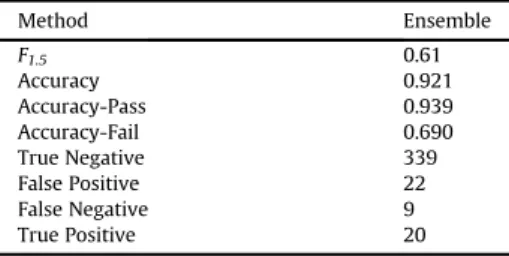
The results of testing the Ensemble model are reported inTable 4andFig. 3. TheF1.5score for the Ensemble model is 0.61, which is higher than all other models. The accuracy of the Ensemble model for students who passed the course is 93.9%, which is lower than the KNN but higher than the SVM and NBC. The accuracy of the Ensemble model for students who failed the course is 69%, which is two times more than the KNN yet lower than the NBC and close to the SVM. The false negative misidentification is only one more than the SVM, which is the second best methods for identifying at-risk students, and the Ensemble method's false positive misidentifications are close to half of the SVM. In addition, most of the misidentifications are C grade students, which is the best possible outcome among the possible errors. However, this method misidentifies one A and three F students.

4.3. Feature selection

Variables were selected based on their correlation to passing/failing the course. In total 14 variables were selected. In addition to the midterm exam grade, 10 out of the 33 learning objective scores and 3 out of the 10 quiz grades were selected. Six out of 10 of the selected leaning objectives relate to user-deﬁned functions in MATLAB, which was the week 5 course topic (seeAppendix Afor more details). Two of the selected learning objectives were related to displaying multiple plots and cumulative distribution plots, and other two were related to exhibiting professional habits.

The accuracy of the models using the feature selection method are reported inTable 5. The models were veriﬁed based on Verify1 dataset. Compared to using all variables, using a subset of variable by feature selection improved the accuracy of the models. The NBC and the Ensemble model were the best models with the highestF1.5scores. The feature selection had a noticeably positive impact on the NBC model. The greatest increase in theF1.5resulted from using the Ensemble method, the

F1.5for the Ensemble models was increased to 0.67. Thus, when using the correlation feature selection method, the Ensemble model was the best model to identify at-risk students.

4.4. Model robustness

After identifying the best modeling methods, the robustness of the selected modeling methods to the size of the training dataset was investigated. Limited data size may result in low accuracy of the models. However, very large training dataset may result in overﬁtting the models to the training dataset and also decreasing the accuracy of the predictions.

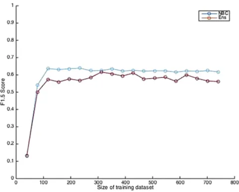
The models were trained with the variables selected from the correlation feature selection method and tested with Verify2 dataset. After the dataset size passed about 120 students, increasing the number of students in the training dataset did not improve the accuracy of the results (Fig. 4). Increasing the size of the training dataset to 780 yielded similar results to 120.

(9)

4.5. Testing the models performance

The performance of the top two prediction models (NBC and Ensemble) at identifying at-risk students in the next se-mester's data was tested. Similar to the previous sections, the models were trained based on the train dataset, which consisted of 780 students from Spring 2013. The test dataset consisted of 1413 students from Spring 2014. The accuracy of the models on this test dataset shows how effective these models are in identifying at-risks students in future semesters.

The course syllabus and grading scheme in Spring 2013 and Spring 2014 were very similar. There were some minor changes from one semester to the other. Some of the instructional team members including instructors and teaching as-sistants were changed from Spring 2013 to Spring 2014. However, the majority of the course syllabus elements were the same between the two semesters. If there were major changes in the course, these models may not be able to identify at-risk students in the subsequent semester with high accuracy.

Table 6shows the accuracy results for the top two models with 14 variables selected by the feature selection method. The NBC model accuracy was higher for students who failed than students who passed. Overall, while the two models performed similarly, the Ensemble model F1.5score was slightly higher than the NBC model. The Ensemble model's accuracy for students

who failed and passed the course was similar. Overall, the Ensemble model was able to identify at-risk students and predict students' success with 85% accuracy.

5. Discussion

The purpose of this study was to compare and_find the best prediction modeling methods among seven different ones and to showcase how to create a course specific prediction model using learning objectives in addition to typical score-based graded assessments. We created course specific prediction models to identify at-risk students at week 5 of the semester in afirst-year engineering course with more than 1600 students. After comparing seven prediction modeling methods, the more accurate ones for identifying at-risk students were the Naive Bayes Classifier (NBC) and an Ensemble model consisting of three models (NBC, Support Vector Machine, and K-Nearest Neighbor). Usually ensemble models have lower error in pre-dicting future data than any of the individual models that make them up (Dietterich, 2000). In this study, NBC performed similarly to the Ensemble model. In this section, we discuss why the NBC and Ensemble models performed better than the other models and why they misidentified some of the students.

From a theoretical perspective, the classiﬁcation error results from bias and variance, and reducing one will result in increasing the other (Williams&Simoff, 2006). Bias is the error due to inaccurate assumptions in the learning algorithm (Hastie, Tibshirani,&Friedman, 2009). Simple models such as those created by the NBC method have higher bias. Variance is sensitivity of the model to small changes, typically due to noise, in the training data. More complex models such as those created by neural networks or decision tree have higher variance (Geman, Bienenstock,_&Doursat, 1992).

In this study, the reasons the NBC model performed better than the other models were that (1) the NBC model has a simple structure and (2) there was a low number of at-risk students in the course. In this study, the NBC calculated the conditional probability of a student being at-risk based on the training dataset, thus the NBC's structure was simpler than other methods. In addition, while the dataset contained a large number of students, a low percentage of students were at risk of failing. In the case of a low training sample size, a simple model with high bias and low variance such as NBC has an advantage over complex models with low bias and high variance such as KNN because the latter will overfit (Sammut&Webb, 2011). Overfitting may occur when the model is complex and has a high variance. In this case, the model does not learn the underlying relations, instead it memorizes the data including the noise in the training data (Everitt&Skrondal, 2002). Thus, an overfit model has high accuracy for training data but low accuracy for future test data.

Considering Logistic Regression modeling as the baseline method, it is possible to divide the modeling methods into two categories: the ones that performed better than Logistic Regression in identifying at-risk students, the SVM and the NBC, and the ones that performed worse than Logistic regression, the KNN, the DT, and the MLP neural network. The methods in each category have two properties in common: bias and variance. As explained earlier, the prediction error is impacted by both bias and variance; decreasing one usually increases the other one (Hastie et al., 2009).

Typically, KNN, DT, and MLP modeling methods result in models with low bias and high variance (Moody, 1994; Olson& Delen, 2008). All three of these models can easily over_ﬁt to the training dataset when the training size is small (Domingos,

Table 4

Test results and accuracy of the Ensemble model.

Method Ensemble F1.5 0.61 Accuracy 0.921 Accuracy-Pass 0.939 Accuracy-Fail 0.690 True Negative 339 False Positive 22 False Negative 9 True Positive 20

(10)

2012). These modeling methods require a large number of training cases to properly be trained. If the number of cases is insufﬁcient (e.g., low number of at-risk students in this study) these models cannot learn the underlying relations in the data and will just memorize the training dataset. Thus, they will have a low accuracy when used to make predictions with other datasets. In contrast, the NBC and SVM modeling methods typically result in models with high bias and low variance (Colas, 2009; Valentini&Dietterich, 2004). Thus, they perform with better accuracy than methods with more complex structures when the sample size does not contain a large number of cases (e.g., number of at-risk students in this study). In summary, because the number of at-risk students in the datasets was low, the simple models with high bias and low variance (i.e., NBC and SVM) performed better than the models with low bias and high variance (i.e., KNN, DT, and MLP). For courses with high student enrollments and a high percentage of at-risk students, the models with more complex structures may perform better than the simple models.

The NBC method is designed based on the naive assumption that the predictor variables are conditionally independent (Duda, Hart,&Stork, 2012). This assumption is used to simplify the calculation of conditional probability in the model. However, NBC typically performs well even if the predicting variables are correlated and this assumption is violated (Bishop, 2006). The NBC model performance may not decrease when there are correlations among predicting variables if the cor-relations, no matter how strong, are evenly distributed in categories (Zhang, 2005). The results of this study are another example of violation of the naive assumption because a student's grades are correlated to each other and not independent, but NBC performed with high accuracy anyway.

Even the more accurate models failed to identify some of the at-risk students. There are multiple reasons why the models could not identify some of the students correctly. First, as statistician George Box said:_“All models are wrong but some are useful”(Box, 1979, p. 209). From a theoretical perspective, in the case of identifying at-risk students, it is not possible to truly model students' success because many factors influence students' behavior and success in a course. Any prediction model is an estimation of students' performance and has its limitations. These limitations will cause the model to misidentify some of the students. In addition, students behaviors are not consistent throughout the semester. For example in this study, the models were trained based on thefirstfive weeks of the semester. It is possible that a student has good performance at the beginning of the semester but begins to perform poorly in the middle or at the end of the semester or vice versa. In either situation, the models are not able to identify this student correctly.

Second, one of the challenging aspects of creating a prediction model for thisﬁrst-year engineering course was the fact that fewer than 10% of the students were at-risk. All prediction modeling methods try to increase the overall accuracy of the predictions. Thus, it is more likely that the created model will perform better for categories with a higher number of cases as compared to the categories with a lower number of cases. Because there were a low number of failing students, most of the models had greater accuracy for students who passed than students who failed.

Fig. 3.Number of Ensemble model misidentiﬁcations.

Table 5

Test results and accuracy of prediction models using feature selection method (14 out of 44 variables selected).

Method Log reg KNN MLP DT SVM NBC Ensemble

F1.5 0.60 0.52 0.56 0.52 0.47 0.62 0.67 Accuracy 0.944 0.928 0.867 0.921 0.954 0.887 0.918 Accuracy-Pass 0.972 0.961 0.873 0.950 1.000 0.889 0.925 Accuracy-Fail 0.586 0.517 0.793 0.552 0.379 0.862 0.828 True Negative 351 347 315 343 361 321 334 False Positive 10 14 46 18 0 40 27 False Negative 12 14 6 13 18 4 5 True Positive 17 15 23 16 11 25 24

(11)

The third reason that the models were not able to identify all students correctly is the limitations of the models caused by pedagogical choices in the course. Thefinal model used the midterm exam grade and one learning objective score. Several factors including the extent to which exam and homework questions assess the desired outcomes in the course, how good these assessments have been designed, and the reliability of grading, influence these variables' ability to predict students success. This ties back to the main goals of backward design (Wiggins_&McTighe, 1998) and standards-based grading (Atwood &Siniawski, 2014). A well-defined learning objective with a designed assessment that is being graded based on a well-defined rubric not only increases fairness and transparency in the course (Sadler, 2005) but also increases the chance to provide a reliable grade with high predictive power for identifying at-risk students.

Fourth and last, in this course only homeworks were graded based on learning objectives; the midterm exam and quizzes were not. The weight of the midterm exam in determining theﬁnal grade was much higher than the individual learning objective scores. Thus, the midterm exam grade was always included in the prediction models. It is possible that not all of the exam questions were good predictors of students' success in the course, but because they were bundled in one single grade, unlike homeworks that assessed 6e7 learning objectives, it was not possible to select the parts of the midterm exam that were better predictors of students success. Therefore, using course performance data including all assessments that are graded based on learning objectives may result in selection of a few midterm learning objectives that can increase the ac-curacy of the predictions.

This study is the next step in the development of early warning systems such as Course Signals (Pistilli&Arnold, 2010) that use generic prediction models. The development of accurate course-speci_fic prediction models in this study con_firms scholars claims (e.g.,Macfadyen&Dawson, 2010) that course-specific prediction models lead to higher accuracy of the predictions. This study also expands on previous research by examining the class size range for which the prediction models can be used. In this study, the accuracy of the predictions reached their best performance after the training dataset contained at least

Fig. 4.Accuracy of the models based on different training size.

Table 6

Test results of top two models using 14 variables selected by the correlation method.

Characteristics NBC Ensemble F1.5 0.59 0.61 Accuracy 0.817 0.846 Accuracy-Pass 0.812 0.848 Accuracy-Fail 0.857 0.830 True Negative 1028 1073 False Positive 238 193 False Negative 21 25 True Positive 126 122

(12)

120 students. The performance of the models stayed almost the same from 120 to 780 students, which was the full training dataset. Thus, it is not clear what the maximum boundary for training the models should be to avoid overtraining the models. Overtraining may occur with a much larger training dataset. In the case of overtraining, the model learns the training data too closely, which may prevent it fromﬁnding the underlying relationships (Nisbet, Elder IV,&Miner, 2009), and the model performs well for the training dataset but very poorly for other datasets (Zaki&Meira, 2014).

The main reason the models performance did not drop with the increase in the size of the dataset is that 780 cases are typically not considered too many for any of the modeling methods, especially when fewer than 10% of students (i.e., fewer than 78 students) belong to one of the categories. A larger dataset is needed to determine the maximum boundary of the modeling methods in identifying at-risk students.

In the training dataset, fewer than 10% of students failed the course, and a subset of 120 students had less than 12 students who were at-risk of failing the course. It is likely that the low performance of the models with datasets smaller than 120 was due to the limited number of at-risk students in the datasets. If a course has a greater number of at-risk students, it may be possible to create prediction models for the course with less than 120 students.

5.1. Limitations and future research

One limitation of this study was due to some of the pedagogical decisions made by the course designers or instructors including the design of the course, the assessments, and the rubrics for grading the assessments. For example, only home-works were graded based on learning objectives. This decision limited the comparability between different forms of assessment in the course including quizzes, homeworks, and midterm exam. In addition, the fact that midterm exam was not graded based on learning objectives prevented us from identifying which sections of the midterm exam were more related to students success in the course.

The models also depend on the performance data that is being collected during the semester. The quality and the reliability of the grading in_fluence the quality of the data and predictive power of the variables, and consequently in_fluence the accuracy of the predictions. If the performance data that is collected during the semester is not valid, it may not be possible to predict students performance at the end of the semester. Students are being evaluated based on these assessments and theirfinal course grade will be based on these performance data. Also the quality and reliability of the data influence any prediction model.

The next logical research step after development of the models is to investigate research questions that can lead to effective use of the prediction models in educational settings. In future research, it may be possible toﬁnd the optimal time to utilize the prediction models during the semester. Predictions made too early may not be very accurate, but late predictions may come when there is too little time to help students. In addition, how the prediction results should be communicated to the students can be investigated. For example, while email notiﬁcations are less time consuming for an instructional team, one-on-one meetings with the students may be more effective.

Other future research might investigate how often the models should be run and students informed about the results. Is it better to inform students weekly, monthly, or only once or twice during the semester? What course topics or learning ob-jectives are most important for students success in a course? While this information may not be shared with the students, instructors can beneﬁt from it and focus on the possible threshold concepts and learning objectives to help students improve their performance. Ethical considerations around the use of such recommendations are also a critical part of potential future research around the results presented in this paper.

6. Conclusion

This study took afirst and successful step in examining different prediction methods for identifying at-risk students early in the semester using performance data during the semester in a course with standards-based grading. For courses with at least 120 students and less than 10% failing rate, it may be possible to use NBC to identify at-risk students during the semester with high accuracy. The more accurate prediction results compared to generic prediction models showcase the possibility of building specific prediction models for each course. In addition to the course-specific models, another aspect of the successful predictions was using in-semester performance data and possibly standards-based grading. Adding this to the already known educational benefits of standards-based grading (although more research is needed) may encourage more instructors to use this kind of grading instead of the traditional score-based grading. All the data that was used in the models, which was in-semester performance data, is available to the course instructors during the in-semester. Thus, by providing specific guidelines on how to create an accurate prediction model (i.e., which prediction model and what types of data to use, how to train, verify, and test the model), course instructors can create and use course-specific models to identify at-risk students and help these students improve their performance.

Appendix A

Homework learning objectives for weeks 1e5 used in the prediction models. Homework LO Description

(13)

(continued)

Homework LO Description

HW01 1 Perform complex calculations using algebraic and trigonometric functions in computations with scalars vectors and matrices HW01 2 Identify appropriate uses for dot notation.

HW01 3 Demonstrate use of colon operator for creating data structures. HW01 4 Demonstrate how to create a MATLAB plot for technical presentation. HW01 5 Demonstrate how to plot multiple data sets on oneﬁgure.

HW01 6 Apply coding standards HW01 7 Exhibit professional habits HW02 1 Use basic relational operators.

HW02 2 Demonstrate the ability to create a histogram for technical presentation. HW02 3 Interpret and evaluate logical statements.

HW02 4 Construct logical statements from English statements. HW02 5 Apply coding standards

HW02 6 Exhibit professional habits

HW03 1 Demonstrate the ability to create a histogram for technical presentation using Excel. HW03 2 Construct cumulative distribution plots in Excel.

HW03 3 Interpret cumulative distribution plots.

HW03 4 Construct and interpret cumulative distribution plots in MATLAB. HW03 5 Construct aﬁgure window to display multiple plots and/or histograms. HW03 6 Apply coding standards

HW03 7 Exhibit professional habits

HW04 1 Interpret cumulative distribution plots (Problem 1).

HW04 2 Generate a histogram suitable for technical presentation from a cumulative distribution plot. HW04 3 Construct cumulative distribution plots in Excel.

HW04 4 Interpret cumulative distribution plots (Problem 2). HW04 5 Construct cumulative distribution plots in MATLAB. HW04 6 Apply coding standards.

HW04 7 Exhibit professional habits.

HW05 1 Construct an appropriate function deﬁnition.

HW05 2 Demonstrate how to create a MATLAB plot for technical presentation. HW05 3 Create a user-deﬁned function using rules for writing functions. HW05 4 Create test cases to evaluate a user-deﬁned function.

HW05 5 Apply coding standards. HW05 6 Exhibit professional habits.

Appendix B

The following are the mathematical descriptions of the prediction models used in this study.

Logistic Regression (Log Reg): Eq.(B1)shows a logistic regression withmpredictor variables (e.g., scores on homework learning objectives, midterm exam, etc.) and one outcome variableY(e.g., probability of passing the course):

Y¼ln p 1p ¼

b

0þ

b

1x1þ

b

2x2þ…þ

b

mxmþe (B1)

wherepis the probability of the desired outcome (e.g., passing the course) based on predictorsx1(e.g., quiz grade) toxm. Support Vector Machine (SVM):The SVM hyperplane can be describe as:

w$Xþb¼0 (B2)

where.

wis the normal to the hyperplane

Xis the vectors of predictor variablesx1toxm b

kwkis the perpendicular distance from the hyperplane to the origin

Toﬁnd the hyperplane with the maximum margin from both categories a Lagrange objective function (Eq.(B3)) should be minimized with respect to thewandbvalues:

(14)

LP¼ 1 2kwk 2Xn i¼1

a

iyðiÞ½xðiÞ$wþb þ Xn i¼1

a

i

a

i>0ci (B3) where.

nis the number of cases (e.g., students)

y(i)is the outcome for casei(e.g., studentipassed or failed) Decision or Classiﬁcation Tree (DT): See section3.4for more detail.

Multi-Layer Perceptron (MLP): Eq.(B4)illustrates a MLP withminput variables and a binary outputy.

y¼sign½fðxÞ where fðxÞ ¼Xm

i¼1

w_ix_iþb (B4)

where.

yis the predicted class (e.g., pass or fail the course) based on predictorsx1toxm.

wiandbare calculated during the training phase.

Naive Bayes Classiﬁer (NBC):Eq.(B5)shows the Bayes conditional probability rule and the naive assumption.

PðCjXÞ ¼PðXjCÞPðCÞ PðXÞ Naive Assummtion: PðXjCÞ ¼ Ym i¼1 Pðx_ijCÞ (B5) where:

P(CjX)is the posterior probability of class C (e.g., pass or fail the course) given predictorsX(e.g., quiz and homework grades);

P(C)is the prior probability of class;

P(xjC)is the likelihood which is the probability of predictor given class;

P(X)is the prior probability of predictor.

A-priori probabilities are calculated based on the training dataset.

K-Nearest Neighbor (KNN):We calculated the Euclidian distance between two points (xandy) tofind the nearest neighbors (Eq.(B6)). dEðx;yÞ ¼ Xm i¼1 ffiffiffiffiffiffiffiffiffiffiffiffiffiffiffiffi x2 i y2i q (B6) References

ACT. (2012).National collegiate retention and persistence to degree rates. fromhttp://www.act.org/research/policymakers/pdf/retain_2012.pdf.

Arnold, K. E., & Pistilli, M. D. (2012). Course signals at Purdue: Using learning analytics to increase student success. InThe 2nd International conference on learning analytics and knowledge, Vancouver, BC, Canada.

Atwood, S. A., & Siniawski, M. T. (2014). Using standards-based grading to effectively assess project-based design courses. InThe american society for en-gineering education annual conference, Indianapolis, IN.

Bishop, C. M. (2006).Pattern recognition and machine learning (Information science and statistics). New York, NY: Springer-Verlag.

Box, G. E. (1979). Robustness in the strategy of scientiﬁc model building. In R. L. Launer, & G. N. Wilkinson (Eds.),Robustness in statistics(pp. 201e236). New York, NY: Academic Press.

Braunstein, A. W., Lesser, M. H., & Pescatrice, D. R. (2008). The impact of a program for the disadvantaged on student retention.College Student Journal, 42(1), 36e40.

Carberry, A. R., Siniawski, M. T., & Dionisio, J. D. N. (2012). Standards-based grading: Preliminary studies to quantify changes in affective and cognitive student behaviors. InIEEE Frontiers in education conference, seattle, WA.

Colas, F. P. R. (2009).Data mining scenarios for the discovery of subtypes and the comparison of algorithms. Leiden University. Cortes, C., & Vapnik, V. (1995). Support-vector networks.Machine learning, 20(3), 273e297.

(15)

DesJardins, S. L., Ahlburg, D. A., & McCall, B. P. (1999). An event history model of student departure.Economics of Education Review, 18(3), 375e390.http://dx. doi.org/10.1016/S0272-7757(98)00049-1.

Dietterich, T. G. (2000). Ensemble methods in machine learning. In J. Kittler, & F. Roli (Eds.),Multiple classiﬁer systems(pp. 1e15). Berlin: Springer. Domingos, P. (2012). A few useful things to know about machine learning.Communications of the ACM, 55(10), 78e87.

Duda, R. O., Hart, P. E., & Stork, D. G. (2012).Pattern classiﬁcation(2nd ed.). New York, NY: John Wiley&Sons.

Eckles, J. E., & Stradley, E. G. (2012). A social network analysis of student retention using archival data.Social Psychology of Education: An International Journal, 15(2), 165e180.

Essa, A., & Ayad, H. (2012). Student success system: Risk analytics and data visualization using ensembles of predictive models. InThe 2nd International conference on learning analytics and knowledge, Vancouver, BC, Canada.

Everitt, B. S., & Skrondal, A. (2002).The Cambridge dictionary of statistics. Cambridge: Cambridge University Press. Field, A. (2009).Discovering statistics using SPSS. Thousand Oaks, CA: Sage publications.

Friedman, J. H., Bentley, J. L., & Finkel, R. A. (1977). An algorithm forﬁnding best matches in logarithmic expected time.ACM Transactions on Mathematical Software (TOMS), 3(3), 209e226.

Gardner, J. N., & Koch, A. K. (2012). Theﬁrst-year experience thirty years Later: It is time for an evidence-based, intentional plan. InPurdue SoLar Flare practitioners' conference, West Lafayette, IN.

Geman, S., Bienenstock, E., & Doursat, R. (1992). Neural networks and the bias/variance dilemma.Neural Computation, 4(1), 1e58. Hand, D. J., Mannila, H., & Smyth, P. (2001).Principles of data mining. New York: MIT press.

Hastie, T., Tibshirani, R., & Friedman, J. (2009).The elements of statistical learning: Data mining, inference, and prediction. New York, NY: Springer. Hendel, D. D. (2007). Efﬁcacy of participating in aﬁrst-year seminar on student satisfaction and retention.Journal of College Student Retention: Research,

Theory&Practice, 8(4), 413e423.

Heywood, J. (2014). The evolution of a criterion referenced system of grading for engineering science coursework. InIEEE Frontiers in education conference, Madrid, Spain.

Huang, S., & Fang, N. (2012). Predicting student academic performance in an engineering dynamics course: A comparison of four types of predictive mathematical models.Computers&Education, 61, 133e145.

James, G., Witten, D., Hastie, T., & Tibshirani, R. (2013).Linear model selection and regularization an introduction to statistical learning. Springer.

Jin, Q., Imbrie, P. K., Lin, J. J. J., & Chen, X. (2011). A multi-outcome hybrid model for predicting student success in engineering. InAmerican society for engineering education annual conference, Vancouver, BC, Canada.

Kutner, M. H., Nachtsheim, C. J., Neter, J., & Li, W. (2004).Applied linear statistical models. Chicago, IL: McGraw-Hill/Irwin.

Kuzilek, J., Hlosta, M., Herrmannova, D., Zdrahal, Z., & Wolff, A. (2015). OU analyse: Analysing at-risk students at The Open University.Learning Analytics Review, 1e16.

Lackey, L. W., Lackey, W. J., Grady, H. M., & Davis, M. T. (2003). Efﬁcacy of using a single, non-technical variable to predict the academic success of freshmen engineering students.Journal of Engineering Education, 92(1), 41e48.

Macfadyen, L. P., & Dawson, S. (2010). Mining LMS data to develop an“early warning system”for educators: A proof of concept.Computers&Education, 54(2), 588e599.

Marbouti, F., Diefes-Dux, H. A., & Strobel, J. (2015). Building course-speciﬁc regression-based models to identify at-risk students. InThe american society for engineering educators annual conference. Seattle, WA.

Meyer, J., & Land, R. (2013).Overcoming barriers to student understanding: Threshold concepts and troublesome knowledge. Routledge.

Moody, J. (1994). Prediction risk and architecture selection for neural networks. In V. Cherkassky, J. H. Friedman, & H. Wechsler (Eds.),From statistics to neural networks(pp. 147e165). Berlin: Springer.

Murtaugh, P. A., Burns, L. D., & Schuster, J. (1999). Predicting the retention of university students.Research in Higher Education, 40(3), 355e371. Nisbet, R., Elder, J., IV, & Miner, G. (2009).Handbook of statistical analysis and data mining applications. Amsterdam: Academic Press.

Olani, A. (2009). Predictingﬁrst year university students' academic success.Electronic Journal of Research in Educational Psychology, 7(3), 1053e1072. Olson, D. L., & Delen, D. (2008).Advanced data mining techniques. Berlin: Springer Science&Business Media.

Pascarella, E. T., & Terenzini, P. T. (2005).How college affects students: A third decade of research. San Francisco, CA: Jossey-Bass.

Pistilli, M. D., & Arnold, K. E. (2010). In practice: Purdue Signals: Mining real-time academic data to enhance student success.About Campus, 15(3), 22e24. Rennie, J. D., Shih, L., Teevan, J., & Karger, D. R. (2003). Tackling the poor assumptions of naive bayes text classiﬁers. InThe 20th International conference on

machine learning, Washington DC.

van Rijsbergen, C. J. (1979).Information retrieval(2nd ed.). London: Butterworths. Rokach, L. (2010). Ensemble-based classiﬁers.Artiﬁcial Intelligence Review, 33(1e2), 1e39.

Romero, C., & Ventura, S. (2010). Educational data mining: A review of the state of the art. Systems, man, and cybernetics, Part C: Applications and reviews. IEEE Transactions on, 40(6), 601e618.

Russell, S., & Norvig, P. (1995).Artiﬁcial intelligence: A modern approach. Englewood Cliffs, NJ: Prentice-Hall.

Sadler, D. R. (2005). Interpretations of criteria-based assessment and grading in higher education.Assessment&Evaluation in Higher Education, 30(2), 175e194.

Sammut, C., & Webb, G. I. (2011).Encyclopedia of machine learning. New York, NY: Springer.

Valentini, G., & Dietterich, T. G. (2004). Bias-variance analysis of support vector machines for the development of SVM-based ensemble methods.The Journal of Machine Learning Research, 5, 725e775.

Wiggins, G., & McTighe, J. (1998).Understanding by design. Alexandria, VA: ASCD.

Williams, G. J., & Simoff, S. J. (2006).Data mining: Theory, methodology, techniques, and applications(Vol. 3755). Berlin: Springer. Zaki, M. J., & Meira, W., Jr. (2014).Data mining and analysis: Fundamental concepts and algorithms. Cambridge: Cambridge University Press.

Zhang, H. (2005). Exploring conditions for the optimality of naive Bayes.International Journal of Pattern Recognition and Artiﬁcial Intelligence, 19(02), 183e198.