İSTANBUL TECHNICAL UNIVERSITY GRADUATE SCHOOL OF SCIENCE ENGINEERING AND TECHNOLOGY
M.Sc. THESIS
JUNE 2016
DICTIONARY ENSEMBLE BASED ACTIVE LEARNING FOR MULTIPLE INSTANCE IMAGE CLASSIFICATION
Gökhan KOÇYİĞİT
Department of Computer Engineering Computer Engineering Programme
Department of Computer Engineering Computer Engineering Programme
JUNE 2016 JUNE 2016
İSTANBUL TECHNICAL UNIVERSITY GRADUATE SCHOOL OF SCIENCE ENGINEERING AND TECHNOLOGY
DICTIONARY ENSEMBLE BASED ACTIVE LEARNING FOR MULTIPLE INSTANCE IMAGE CLASSIFICATION
M.Sc. THESIS Gökhan KOÇYİĞİT
504121547
Bilgisayar Mühendisliği Anabilim Dalı Bilgisayar Mühendisliği Programı
HAZİRAN 2016
İSTANBUL TEKNİK ÜNİVERSİTESİ FEN BİLİMLERİ ENSTİTÜSÜ
ÇOKLU ÖRNEKLİ GÖRÜNTÜ SINIFLANDIRMASI İÇİN SÖZLÜK TOPLULUĞU TABANLI AKTİF ÖĞRENME
YÜKSEK LİSANS TEZİ Gökhan KOÇYİĞİT
504121547
v
Thesis Advisor : Asst.Prof.Dr. Yusuf YASLAN ... Istanbul Technical University
Gökhan KOÇYIĞIT, a M.Sc. student of İTU Graduate School of Science Engineering and Technology student ID 504121547, successfully defended the thesis/dissertation entitled “DICTIONARY ENSEMBLE BASED ACTIVE LEARNING FOR MULTIPLE INSTANCE IMAGE CLASSIFICATION”, which he prepared after fulfilling the requirements specified in the associated legislations, before the jury whose signatures are below.
Date of Submission : 02 May 2016 Date of Defense : 07 June 2016
Jury Members : Assoc.Prof.Dr. Songül ALBAYRAK ... Yıldız Technical University
Assoc.Prof.Dr. Şule Gündüz ÖĞÜDÜCÜ ... Istanbul Technical University
vii
ix FOREWORD
First of all, I would like to thank my supervisor Asst. Prof. Dr. Yusuf YASLAN. Without his guidance and relentless support for my research, I couldn’t finish my thesis. He encouraged me and helped me when I encountered difficulties. I also would like to express my gratitude to the Turkish Naval Forces for this opportunity. Also, I would like to thank my mother and father for supporting me whatever I do. Last, but not least, I thank my spouse for being by my side at all times.
June 2016 Gökhan KOÇYİĞİT
xi TABLE OF CONTENTS Page FOREWORD ... ix TABLE OF CONTENTS ... xi ABBREVIATIONS ... xiii SYMBOLS ... xv
LIST OF TABLES ... xvii
LIST OF FIGURES ...xix
SUMMARY ...xxi
ÖZET ... xxiii
1. INTRODUCTION ...1
1.1 Contribution of the Thesis ...2
1.2 Thesis Structure ...3 2. BACKGROUND ...5 2.1 Multiple-Instance Learning ...5 2.1.1 Instance-space algorithms ...6 2.1.2 Bag-space algorithms ...7 2.1.3 Embedded-space algorithms ...8 2.2 Classifier Ensembles ...9
2.2.1 Creating the classifier ensemble ... 10
2.2.2 Combining the ensemble results ... 11
2.3 Sparse Coding ... 13
2.3.1 Definition ... 13
2.3.2 Greedy approaches ... 14
2.3.3 Relaxation techniques ... 15
2.4 Dictionary Learning ... 15
3. DICTIONARY ENSEMBLE BASED MULTIPLE INSTANCE LEARNING ... 19
3.1 Dictionary Ensemble Based MIL Algorithm ... 19
3.2 Experimental Setup ... 21
3.3 Experimental Results ... 23
4. DICTIONARY ENSEMBLE BASED MULTIPLE INSTANCE ACTIVE LEARNING ... 25
4.1 Active Learning ... 25
4.2 Multiple Instance Active Learning ... 26
4.3 Dictionary Ensemble Based Multiple Instance Active Learning ... 28
4.4 Experimental Results ... 31
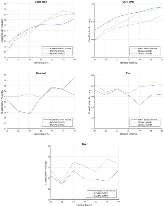
4.4.1 Comparing with the kernel-based MI active learning method... 32
4.4.2 Comparing the base classifiers with different query strategies ... 34
5. CONCLUSION AND FUTURE WORK ... 37
REFERENCES ... 39
APPENDICES ... 43
xiii ABBREVIATIONS
MIL : Multiple Instance Learning MI : Multiple Instance
IS : Instance-Space
BS : Bag Space
ES : Embedded-Space
APR : Axis-Parallel Rectangle DD : Diverse Density
EM : Expectation-Maximization EMD : Earth Movers Distance SVM : Support Vector Machine DT : Decision Tree
MLP : Multi-Layer Perceptron
NP-Hard : Non-deterministic Polynomial-time Hard MP : Matching Pursuit
OMP : Orthogonal Matching Pursuit LARS : Least Angle Regression MOD : Method of Optimal Directions SVD : Singular Value Decomposition
SCCE-MIL : Sparse Coding and Classifier Ensemble based Multiple Instance Learning
DEMIAL : Dictionary Ensemble based Multiple Instance Active Learning KKT : Karush-Kuhn-Tucker conditions
xv SYMBOLS
, { }, { } : The ith bag in all dataset, training set and unlabeled set respectively
, { }, { } : Number of examples in all dataset, training set and unlabeled set respectively
: Number of instances in the ith bag : Number of classes in the dataset : The ith bag label
: The jth instance in the ith bag
: The probability of the instance in DD algorithm
, : The minimal Hausdorff distance between two bags
, : The Earth Mover Distance between two bags
, : Set kernel value between two bags
, : Normalized set kernel value between two bags : The ith bag feature vector
: Ensemble size
, : Decision of the ith classifier of the class j : Weight of the ith classifier
! " : Ensemble support value of the class k
# : Instance matrix
: Number of instances in the instance matrix : Dictionary
$ : Sparse representation of the ith instance
% $ : Regularization function
: The jth atom in the dictionary D & : Residual energy of the signal with dj0 ∗ : Queried bag in active learning
() | : Posterior probability under the model θ given bag
i B
xvii LIST OF TABLES
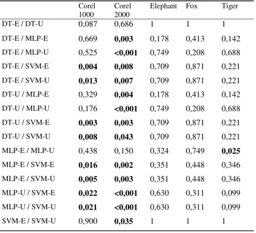
Page Algebraic ensemble combiners. ... 12 Table 3.1 : SCCE-MIL algorithm. ... 21 Table 4.1 : DEMIAL algorithm. ... 31 Table 4.2 : p-values for DEMIAL algorithm with respect to base classifier and query strategies using paired t-test. ... 36
xix LIST OF FIGURES
Page The difference between single instance learning and multiple instance
learning. ...5
Figure 3.1 : Overview of SCCE-MIL algorithm. ... 20
Figure 3.2 : Example images of COREL 1000 dataset [11]. ... 22
Figure 3.3 : Result of the SCCE-MIL algorithm with different ensemble size and base classifier. ... 24
Figure 4.1 : Overview of the proposed DEMIAL algorithm. ... 29
Figure 4.2 : Comparison between DEMIAL and kernel based MI active learning algorithm. ... 33
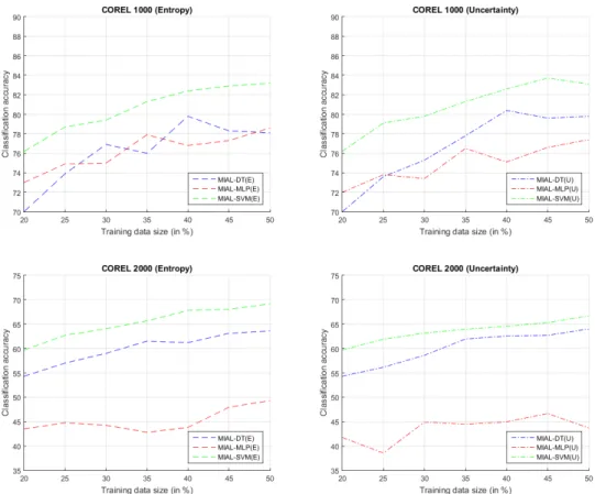
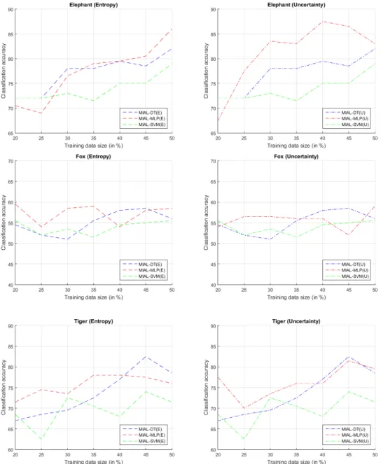
Figure 4.3 : Comparison of the base classifiers in DEMIAL algorithm with entropy and uncertainty query strategy. ... 34
Figure A.1 : Example of support vectors, decision boundary and margins [39]. ... 44
Figure A.2 : Example of a multi-layer perceptron with one hidden layer [39]. ... 46
xxi
DICTIONARY ENSEMBLE BASED ACTIVE LEARNING FOR MULTIPLE INSTANCE IMAGE CATEGORIZATION
SUMMARY
In a machine learning problem, each data sample is represented with a feature vector and associated with class information. As an extended version of this approach, in a Multiple Instance Learning (MIL) problem, each data sample consist of a set of feature vectors which may represents the part of the whole entity. Lately, MIL framework draws a lot of attention due to its suitability to the real-world problems e.g. image categorization. In that sense, with the popularity of the internet, it is easy to acquire large collection of data. Using large quantity of data in a MIL setting requires labeling process for each data sample which is a laborious task to accomplish. To overcome this problem, active learning can be used. Active learning is an iterative framework which selects best representative data samples to be labeled by an oracle. In the literature there are several approaches that combine the MIL framework with active learning. Recently sparse coding techniques which approximate a given signal by combining few redundant basis vectors have been applied to MIL framework. In this thesis, we developed an MI active learning method that corporates with sparse coding and classifier ensemble technique called DEMIAL (Dictionary Ensemble based MI Active Learning). The proposed DEMIAL algorithm constructs the classifier ensembles on the sparse feature sets that are obtained from multiple sized dictionaries. The experimental results are obtained on 5 different popular image categorization MIL datasets. Initially we obtained supervised learning results on these datasets with using different base classifiers and ensemble sizes. Then the DEMIAL algorithm is compared with kernel based MI active learning method using two different active learning selection strategies. The effect of the base classifiers and active learning strategies are also considered for DEMIAL algorithm. It is shown that the proposed DEMIAL algorithm performs better than the kernel-based MI active learning method.
xxiii
ÇOKLU ÖRNEKLİ GÖRÜNTÜ SINIFLANDIRMASI İÇİN SÖZLÜK TOPLULUĞU TABANLI AKTİF ÖĞRENME
ÖZET
Makine öğrenmesi, öğrenilecek verinin geçmiş bilgisini kullanarak modelleyen ve daha sonrasında elde edilecek yeni veriler için karar veren yöntemler bütünüdür. Günümüzde teknolojinin gelişimi ile birlikte çok büyük miktarda veri üretilmekte ve buna bağlı olarak makine öğrenmesi ile bu veriler ve bunlara bağlı problemlerin çözümü için çok çok sayıda çalışma ve araştırma yapılmaktadır. Bu çözümlerin temelinde, öğreneceğimiz verinin modellenmesi yatmaktadır. Veriler genellikle öznitelik vektörleri ve onunla ilişkilendirilmiş sınıf etiketleri ile gösterilmektedir. Fakat bazı problemlerde bir veri birden fazla öznitelik vektörüne sahip olabilir. Böyle bir durumda modelleme işleminin birden fazla özellik vektörü ile yapılması gerekir ve bu modelleme tekniğine Çoklu Örnek Öğrenme denilmektedir.
Çoklu Örnek Öğrenme, başlangıçta ilaç molekül aktivitelerinin yapısını öğrenebilmek için ortaya atılmış olsa da, son zamanlarda metin sınıflandırma, görüntü çağrılması vb. gibi çok farklı makine öğrenmesi problemlerine de uygulanmaktadır. Temelde, bir veriye ait birden fazla öznitelik vektörleri bulunmaktadır ve her bir özellik vektörüne örnek, veriye ait bütün örneklerin birleşimine de torba denilmektedir. Çoklu Örnek Öğrenme sisteminde verilerin sınıf etiketlerinin bilgisi torbayla ilişkilendirilmiş olup örneklerin etiket bilgisi bulunmayabilir. İkili sınıflandırma problemi ele alınırsa, torba içerisindeki en az bir örnek eğer pozitif ise torbanın tamamı pozitif olarak sınıflandırılmaktadır. Eğer bütün örnekler negatif ise, torbanın sınıfı negatif olmaktadır.
Çoklu Örnek Öğrenme için önerilmiş algoritmaları üç sınıfta incelemek mümkündür. Bunlardan birincisi örnek uzayını kullanan yöntemler olarak nitelendirilmektedir. Örnek uzayında sınıflandırıcılar sadece örnekler üzerinde çalıştırılmaktadır. Bu tip yöntemlerdeki genel mantık, pozitif özellikli örneklerin negatif özellikli örnekler ile ayrışmasını sağlayarak yeni gelecek verilerdeki örneklerin sınıflandırmasıdır. Fakat örnek uzaydaki sınıflandırıcılar torbayı tamamen ele alıp öğrenme yapmadıkları için torbanın genel yapısını öğrenemezler. Ayrıca, bazı uygulamalarda torbaya ait her bir örneğin sınıf bilgisi bulunmadığından örnekler üzerinden öğrenme işlemi yapılamamaktadır. Bu problemleri ortadan kaldırmak için torba uzayında sınıflandırıcı öğrenen yöntemler önerilmiştir. Torba uzayında çalışan sınıflandırıcılar her bir örneği teker teker değerlendirmeyip torbayı bir bütün olarak değerlendirmektir. Bu tekniklerde genelde dikkat edilecek husus, torba verisinin vektörel olmayan yapısıdır. Bu şekildeki yapıların sınıflandırıcı tarafından öğrenilmesi için iki torbayı karşılaştıran bir fonksiyon gereklidir. Bu fonksiyon dolaylı olarak iki torbayı karşılaştırıp sonuç vermektedir. Fakat torbanın vektörel olmayan yapısı nedeniyle, geliştirilen yöntemlerin karmaşıklığı normal sınıflandırıcılara göre yüksek ve daha zaman alıcıdır. Bununla birlikte, öğrenilmeye çalışılan eniyileme fonksiyonunun konveks olmaması nedeniyle yerel minimum problemi yaşanabilmektedir. Bu problemleri aşmak için üçüncü bir teknik olarak,
xxiv
gömülü uzayda öğrenen sınıflandırıcılar önerilmiştir. Bu sınıflandırıcılardaki temel mantık, veri tabanındaki her bir torbanın örnekleri bir fonksiyon yardımıyla doğrudan tek bir öznitelik vektörüne dönüştürülerek, elde edilen torba vektöründen makine öğrenmesinde kullanılan bilindik yöntemlerle öğrenmesini sağlamaktır. Gömülü uzaydaki yöntemin başarısı torbaların torba vektörüne dönüşümünde kullanılan fonksiyonun seçimine bağlıdır. Dönüşüm işlemini kolaylaştırmak ve verinin örüntüsünü ortaya çıkarmak için kullanılan yöntemlerden birisi seyrek kodlamadır.
Seyrek kodlama, sinyal işleme ve görüntü işleme toplulukları tarafından son zamanlarda çokça kullanılan bir yöntemdir. Bunun nedeni, seyrek kodlanacak verinin, sözlük denilen ve veriyi temsil eden temel matrisin içerisindeki temel vektörlerin çok azının doğrusal katışımıyla elde edilebilmesinden dolayıdır. Bu gösterimin faydası, veri için üst düzey bir gösterim sağlayarak verinin örüntüsünü ortaya çıkarmaktadır. Seyrek kodlama için önceden belirlenmiş temel matrisler kullanılmakla birlikte son zamanlarda yapılan çalışmalar ile temel matrisin veriden öğrenilmesinin daha iyi sonuç verdiği görülmüştür. Seyrek kodlama işlemindeki temel matrise sözlük denilmekte ve bu temel matris çıkarım işlemine ise sözlük öğrenimi denilmektedir.
İnternetin yaygınlaşmasıyla birlikte büyük verilere erişim çok kolaylaşmıştır. Fakat, büyük verilerin makine öğrenmesi tekniklerinde kullanılabilmesi için her bir verinin sınıf etiketinin belirlenmesi gereklidir. Bu işlem bazı uygulamalar için çok zaman alıcı veya pahalı bir işlem olabilmektedir. Bunun yerine, etiketsiz veri tabanından akıllıca seçim yapılarak sadece seçilenlerin etiketlerinin elde edilmesi gerçeklenebilir. Literatürde bu tekniğe aktif öğrenme denilmektedir. Aktif öğrenme sisteminde, sınıflandırıcı etiketsiz verilerden kendisine en fazla bilgiyi verecek olanları seçerek sınıf bilgisinin öğrenilmesi için bir uzmana danışır. Uzmanın verdiği sınıf bilgisi ile birlikte bu veri öğrenme verisine eklenir ve sınıflandırıcı yeni veri ile birlikte güncellenir. Bu işlem önceden belirlenmiş bir yineleme sayısı kadar tekrar eder. Öğrenme verisinin en son hali ile de son sınıflandırıcı öğrenilir.
Son zamanlarda, çoklu örnek öğrenme ve aktif öğrenme sistemleri birleştirilerek çoklu örnekli aktif öğrenme metotları geliştirilmiştir. Bu metotlar çoklu öğrenmenin hangi uzayda yapıldığına göre değişim göstermektedir. Bu yüzden çoklu örnekli aktif öğrenme metotları torba uzayında ve örnek uzayında yapılabilmektedir. Fakat bildiğimiz kadarıyla gömülü uzayda çalışan çoklu örnekli aktif öğrenme metodu üzerine çalışma yapılmamıştır. Bu tezde, seyrek kodlama ve sınıflandırıcı topluluğu tekniklerini kullanan çoklu örnekli aktif öğrenme metodu, DEMIAL algoritması önerilmiştir.
Önerilen DEMIAL algoritması genel olarak 5 farklı adımdan oluşmaktadır. Öncelikle, öğrenme verisi kullanılarak birbirlerinden farklı boyutlardan oluşan farklı sözlükler öğrenilmektedir. Bunun amacı, farklı boyutlarda öğrenilen sözlükler ile sınıflandırıcı topluluğu oluşturulup, topluluk içerisindeki çeşitliliği sağlamaktır. Daha sonra elde edilen sözlükler ile seyrek kodlama yapılarak torba içerisindeki örneklerin seyrek gösterimleri elde edilir. Seyrek kodlama örneklere üst düzeyde bir gösterim sağladığı için kullanılmıştır. Daha sonra torbaya ait örneklerin seyrek gösterimleri, birleştirilerek her bir torbanın öznitelik vektörü oluşturulur. Kullanılan birleştirme fonksiyonu örneklerin seyrek gösterimlerini özetleyen bir fonksiyon olup, örneklerin tamamını temsil eder. Öğrenme aşamasında ise torba özellik vektörleri kullanılarak makine öğrenmesinde kullanılan sınıflandırıcılardan birisi kullanılır. Bu aşamaya kadar yapılan işlemler Eğiticili Çoklu Örnek Öğrenme adımlarıdır.
xxv
Önerilen DEMIAL algoritmasının aktif öğrenme aşamasında, etiketsiz verilerin seyrek kodlaması yapılır ve her bir veri tek bir torba vektörüne dönüştürülür. Daha sonra etiketsiz veri üzerinde torba vektörü kullanılarak sınıflandırıcılardan sınıf bilgisi öğrenilir. Sınıflandırıcı topluluğunun kararı ile en yararlı veri seçilir ve uzmana sorularak sınıf bilgisi alınıp öğrenme verisine eklenir. Bu işlem belirli bir tekrarlama ile devam eder ve en sonunda son kez öğrenme verisinden sınıflandırıcı öğrenilir.
Deneysel sonuçlar 5 farklı Çoklu Örnek Öğrenme problemi içeren görüntü sınıflandırma veri kümelerinde elde edilmiştir. Öncelikle Eğiticili Çoklu Örnek Öğrenme algoritması olan SCCE-MIL yöntemi, farklı boyutlardaki sınıflandırıcı toplulukları ve farklı baz sınıflandırıcılar kullanılarak incelenmiştir. Daha sonra önerilen DEMIAL algoritması çekirdek tabanlı çoklu örnekli aktif öğrenme algoritmasıyla farklı aktif öğrenme sorgu yöntemleri ile karşılaştırılmıştır. Ayrıca baz sınıflandırıcıların DEMIAL algoritmasının başarımına olan etkileri de incelenmiştir. Deneysel sonuçlarda önerilen DEMIAL algoritmasının daha iyi sınıflandırma başarımına sahip olduğu görülmüştür.
1 1. INTRODUCTION
Machine Learning is a framework that models a given task by utilizing the past experience or the example data. Learning problems often comes where we cannot explicitly write a computer program about the given task. This process is an operation of optimizing a hypothesis for the given task which is called learning. After the learning, this hypothesis is used for prediction on new instances.
Machine learning techniques are mainly separated into 3 categories. First category is called supervised learning in which, the training data is given with category information namely label. Using these labels, we generalize the class information by a model to be able to identify the new example. This method is also referred as classification.
The second category in the machine learning is called unsupervised learning. In unsupervised learning, the training data has no label information and the aim is to find any pattern or information from how data is composed. Finding any pattern in data may be a challenging task than the supervised learning but it is essential for some applications where we can’t receive any label information.
In many domains, obtaining data is cheap but labeling them can be laborious. Therefore, one can obtain few labeled data and huge amount of unlabeled data samples. These types of applications are named as semi-supervised learning which is the combination of the supervised and unsupervised learning. Essentially, training is done by both labeled and unlabeled data. In general, learning with unlabeled data incorporated with some labeled examples improves the learning accuracy. This is also helpful for some applications where obtaining the label information is difficult and expensive.
Essentially, the above categories only deal with data samples which have one input feature vector. But there are many applications where the data has multiple features that represent a given data. Learning process of those data is called Multiple-Instance Learning (MIL) which is an extended version of supervised learning. In MIL
2
framework, each data sample consists of bag - which is a collection of feature vectors called instances - and class labels are associated with bags. In some applications MIL offers a better representation of a real-world problem more than the standard supervised learning. For example, in image categorization, a single image is represented as a single feature vector in supervised learning. However, in the MIL settings, we can represent a single image with set of feature vectors which are extracted from separated regions of the image.
Nowadays with the advance of the technology, it becomes easy to obtain a vast amount of unlabeled data. In order to use this abundant data in a supervised learning framework, each data sample has to be labeled manually which can be an overwhelming task to accomplish. Instead of labeling all the unlabeled data, one can “smartly” select some of them using an active learning framework. Active learning is a well-known and widely used framework for many machine learning problems where obtaining data labels are difficult and expensive. In this framework, active learner is allowed to choose the most informative unlabeled data and ask (query) its label from the oracle to perform better with less training data.
In order to combine the MIL framework and the active learning framework, we need to represent the instances in the bags more efficiently so that the classifiers have better results. This can be achieved with sparse coding techniques. Sparse coding is a well-known technique in signal processing and image processing communities which allow us to represent signals with the linear combination of the basis vectors called atom and the collection of the atoms are called dictionary. This technique gives us a general representation of a signal in terms of sparse combinations of atom vectors. Also, sparse coding removes the possible noise from the signal.
In this thesis, we propose an MI active learning method, namely DEMIAL (Dictionary Ensemble based Multiple Instance Active Learning), which employs classifier ensembles that is trained in sparse represented data. We compare our method with different ensemble techniques, ensemble combination methods.
1.1Contribution of the Thesis
This thesis composed of four different aspects which bring novelty to the MIL framework:
3
- We propose an MI active learning approach using classifier ensemble system which is trained with a sparse representation of the data from the multiple different sized dictionaries.
- We analyze the active learning query strategies for the proposed algorithm and compare these with different approaches in the MIL framework.
- Ensemble system is constructed by using different sized dictionaries in which ensemble size is investigated.
- DEMIAL algorithm is investigated with different base classifiers and active learning query strategies for image categorization.
1.2Thesis Structure
The remaining chapters of the thesis are as follows. In Chapter 2, we cover the methods and techniques that are used in this thesis as background information. In Chapter 3, we will discuss the MIL framework with sparse coding and classifier ensemble methods. In Chapter 4, we will present the, DEMIAL, MI active learning method with sparse coding and classifier ensemble. In Chapter 5, we will conclude the thesis by giving the take home messages.
5 2. BACKGROUND
In this chapter, we will cover some of the previous works about MIL and other methods that are used in this thesis.
2.1Multiple-Instance Learning
Multiple-Instance Learning is a machine learning framework proposed by Dietterich et al [1]. In MIL framework, each sample in a dataset is a set of feature vectors representing a sub-part of the sample itself called instances. If we rephrase the last statement in MIL terms, each data sample in the dataset is a bag of instances. Each bag has a class information in the dataset and instances may have a class association but may not be known. In binary classification, a bag is considered positive if at least one of the instances is positive. If all the instances are negative, then the bag label is negative. The MIL framework is represented in Figure 2.1.
The difference between single instance learning and multiple instance learning.
6
Mathematically, each bag in the dataset can be shown as + = - ., /, … , 123 where is the jth instance vector of the ith bag. Class information is represented as
4 and it is associated with the +. Note that each bag has a different number of instances which is denoted as 5. For binary classification, 4 becomes positive if at least one instance in + is positive. If all the instances in the bag are negative, then 4 considered as negative.
To solve MIL problems, there are several approaches in the literature. Mainly, MIL approaches are separated in three categories: Instance-Space (IS), Bag-Space (BS) and Embedded Space (ES) [2]. We will investigate these categories more detail in the following sub-sections.
2.1.1 Instance-space algorithms
Algorithms that use only instances in the bags are considered instance-space (IS) algorithms. In the IS algorithms, label information is considered as related to instances and classifiers are trained by positive instances in the bags.
Multiple-Instance Learning was firstly proposed by Dietterich et al. [1] for the prediction of drug molecule activity. In their work, they proposed the first MIL method named Axis-Parallel Rectangle (APR) algorithm which builds a hyper-rectangle around the positive instances of each bag while not including the negative instances.
After that, Maron et al [3] proposed the diverse density (DD) algorithm for MIL framework. Unlike the APR algorithm which encloses the instances with a hyper-rectangle in the instance-space, DD algorithm tries to find a single vector in the instance space that has minimum distance with the positive instances while has maximum distance with the negative instances. Mathematically, the classifier is a vector ℎ = {7}, 7 ∈ ℝ: and the posterior probability of the instance given the features depends on the distance between it and the classifier vector:
; = exp ?−A − 7A/B (2.1)
Specifically, they defined a positive region with a Gaussian centered vector 7 with this probability. To calculate this region, they defined an optimization function with all of the positive instances fall in the region and the negative ones are out of it. This
7
optimization is done with a noisy-OR model for calculating the likelihood of the data sample and the gradient descent for training the optimal classifier vector [4].
Following the same principle, Zhang and Goldman [5] has proposed EM-DD algorithm which uses Expectation–Maximization (EM) algorithm for the DD optimization. The EM-DD, algorithm first estimates the most probable instances in the bags to have the positive label. Then according to its predictions, it finds the classifier vector which has the maximum distance between the negative instances and minimum distance between the positive instances. This process will continue until no further improvement is achieved or a predefined set of iterations.
Alternatively, Andrews et al [6] proposed mi-SVM algorithm which uses only instance information. In their algorithm, the goal is to find an MI-separating hyperplane which separates at least one positive instance and thus creates halfspace of positive and negative instances.
2.1.2 Bag-space algorithms
In instance-space, algorithms train a model to estimate instances’ labels and discriminate the positive instances against the negative instances. Thus, this type of algorithms train on local information. In contrast, bag-space algorithms train a model using the bags and this allows the algorithm to capitalize more information especially bag information.
Since the bags are non-vector entity, we have to define a function which compares two bags in the dataset. Usually, comparison function calculates the distance of the two bags + and +C. In the literature there are several different distance functions that are used in MIL settings. One of them is the minimal Hausdorff distance [7]:
DE + , +C =I min
2J∈K2,ILM∈KLA − CNA (2.2) This function gives the minimum distance between two bags’ instances. The other distance function is Earth Movers Distance (EMD) [8] :
OPE + , +C =∑ ∑ 7N∑ ∑ 7NA − CNA N
8
where 7N are the weights of the instances that are calculated by an optimization process which minimizes the OPE + , +C with some constraints.
Aside from the distance functions, kernel functions are also used as a similarity measure. Thus one can benefit from the advantages of kernel functions. Gartner et al. [9] has proposed set kernel function:
5STU + , +C = V W , CN
I2J∈K2,ILM∈KL
(2.4) where W . , . is any kernel function e.g. Gaussian, polynomial, linear, etc. that uses instances and CN as the input. To overcome the varying cardinality of the instances the set kernel similarity is normalized using the following formula:
5YSTU + , +C = 5STU + , +C
Z5STU + , + Z5STU +C, +C (2.5)
2.1.3 Embedded-space algorithms
Embedded-space algorithms are similar to the bag-space algorithms. In Bag-space, the bag features are constructed by using distance or kernel functions implicitly. In Embedded-space algorithms, bags are converted into a single feature vector explicitly by using a mapping function.
In that sense, Gartner et al [9] proposed a statistic kernel which aggregates the instances in a statistical approach. The intuition of the statistic kernel (which is also called pooling function in some other areas) is to summarize the bag into a single representative vector by using statistics e.g. mean, median, min-max etc. This technique allows us to use different statistics about the data. As an example to the pooling function, max pooling function can be given as follows:
+[ W = max-| . W |, | / W |, … , ] W ], … 3 (2.6)
where +[ W is the kth element of the ith bag feature and W is the kth element of instance .
Alternatively, Chen and Wang [10] proposed DD-SVM method that combines the DD method and Support Vector Machines (SVM). This algorithm has two steps: 1)
9
calculate the instance prototypes using the DD algorithm, 2) each bag is mapped into a new feature space using the learned instance prototypes. Then they trained a SVM using these new features. Similar to DD-SVM, Chen et al. [11] proposed MILES algorithm that extends the DD method. Their approach is to calculate the instances that are close to classes by embedding the instances and selecting the features that are most relevant.
2.2Classifier Ensembles
In the real world, we often find ourselves with a decision which we can’t decide it by ourselves. At that time, we usually obtain other people’s opinion and combine their decisions with our’s. This natural process can be applied to the machine learning framework in which training multiple classifiers and combining the decisions of them is called classifier ensemble system. By combining classifiers, our aim is to achieve more accurate classifier system than a single classifier which reduces the possibility of a wrong classification [12].
Another aspect of a classifier ensemble is the usability with too large size of instance space. In some applications, large amount of the data has to be learned for an effective classifier but data size makes the learning process not practical to be handled by a single classifier. This problem can be solved by constructing a classifier ensemble in which, each classifier is trained with the subset of the whole dataset. This solution is proved to be much more efficient approach rather than the single classifier trained on the whole dataset [13].
Similarly, to the size of the dataset, there are some applications in which each data sample has large feature vector. These kinds of applications become troublesome for single classifiers because complexity of the learning process is getting higher with more features which is called curse of dimensionality problem. To solve this, an ensemble system can be constructed with classifiers learned with the subspaces of the feature vector. This technique allows us to select some features in the dataset and discards the others which reduce the complexity of the learning algorithm.
Another problem with a single classifier is that the data sample can be too complex for a single classifier to solve by itself. Specifically, for a given dataset, decision boundary of the data can be too complex for the classifier to fit. These complex
10
boundaries can be approximated by dividing the data into sections and training a classifier for each section and combining the results. This divide-and-conquer-like strategy is appropriate for much more complicated problems.
Ensemble system is useful for many applications. But this requires classifiers to be diverse in their decisions to boost the overall classification. To be more specific, each classifier should make different errors so that combination of the classifiers reduces the total error. This means that each of the classifier doesn’t have to be the best to classify the data by itself but the combination with the other classifiers achieve better results [12].
All classifier ensemble systems have two important functions that we build ensemble system upon. One of them is creating a set of classifiers that are diverse enough and the other one is the combination of the results. We will discuss these functions in following sub-sections.
2.2.1 Creating the classifier ensemble
In order to create an ensemble system, we have to find a way to generate multiple base classifiers which are different enough from each other. There are several methods in the literature for creating diverse ensemble system.
One of the early and most used approach for ensemble system is called bootstrap
aggregating (or in short bagging) in which, different data subsets are randomly
selected from the whole training dataset. Each subset of the data is used for training a single classifier. But using random selection technique would yield duplicate data on multiple subsets of the dataset with probability of approximately 0.368. To create diversity in bagging, unstable base classifiers, in which small changes in the dataset would yield larger output changes e.g. decision tree and multi-layer perceptron, is recommended [13].
Alternative to the bagging, boosting is proposed by Schapire [14] which generates weak classifiers but the combinations of them make strong learner. Boosting also uses resampling of the data but selects with a strategy. The classifiers that use subset of data are created iteratively. At first, classifier is trained by randomly selected subset data. For the next classifier, the most informative data is selected given the first classifier and trained accordingly. The third classifier’s data is selected which first and second classifier disagree [12].
11
As a more general approach, AdaBoost is proposed by Freund and Schapire [15]. In AdaBoost, for each classifier in the ensemble, data samples are selected with an iteratively updated distribution. In this distribution, the likelihood of the given data sample is increased when it is misclassified. This ensures that in the next iteration misclassified data is used most probably for the training.
Another approach for diverse ensemble is to adjust the training parameters of the classifier so that each classifier’s decision boundary differs from each other. Training parameters control the instability of the classifier and thus the diversity can be achieved [12]. Lastly, diverse ensembles can be constructed by training classifiers that uses different feature subsets of the data. This method is called random subspace method [16].
2.2.2 Combining the ensemble results
The second most important function for ensemble system is combining the results of the multiple classifiers for a given data. The result of the ensemble depends on the decisions given by the classifiers. Since we assume that classifiers’ results are different enough from each other, combination strategy is crucial for ensemble system. In general, there are two group of combination strategies: combination of class labels and combination of class posterior probabilities.
There are several methods for combining the class labels. The straightforward method would be to classify the data with the label on which majority of the classifiers agree. This method is called majority voting and can be described as,
V ^,C _ `. = max`.…aV ^, _ `. (2.7)
where ^, is the binary decision of the ith classifier about the class j, b is the ensemble size and W is the chosen class. Note that majority voting can be used under some assumptions: 1) b has to be odd, 2) probability of each classifier i to give the correct class label is equal for any data and 3) classifier outputs are independent of each other [13].
If we have a prior knowledge that some classifiers are somewhat more competent than other classifiers, we can weight their outputs and combine them. This technique
12
is called weighted majority voting and can be shown as,
V 7 ^ ,C _ `. = max`.…aV 7 ^, _ `. (2.8)
where 7 is the weight of the ith classifier. For this technique, the most important problem is to assess the classifiers quality and weight their contribution. If we have the prior knowledge of the classifiers performance, it won’t be a problem. But if we don’t have, we have to come up with a strategy. In some ensemble techniques like AdaBoost, the assessment is made while the ensemble is constructing. For others, we can split a validation dataset and assess the classifiers performance on it.
Beside class labels, classifiers may have a continuous output that shows the likelihood of a given class. For the combination of the class likelihoods, there are several methods in the literature but the most common used ones are called algebraic combinations. The outputs are combined in an algebraic function that supports the best results. These functions are represented in Table 2.1.
Algebraic ensemble combiners.
Name Formula Product Rule cC d =1 b f ^,C d _ `. Mean Rule cC d =1 b V ^,C d _ `.
Max Rule cC d = max`.…_-^,C d 3 Median Rule cC d = median`.…_ -^,C d 3 Minimum Rule cC d = min`.…_-^,C d 3 Weighted Average cC d =1
b V 7 ^,C d
_ `.
Each function leverages some quality of the outputs and some functions are more suitable for some ensemble techniques. For example, for AdaBoost, weighted average is more suitable since the algorithm calculates the weights of the classifiers.
13
The best combination method depends on the problem and our prior knowledge of the problem [12].
2.3Sparse Coding
In signal processing, sparse coding is a well-known technique to approximate a given signal by combining few redundant basis. The advantage of the sparse coding is that signals can be well approximated and the resulting sparse features capture the structures or patterns of the signals [17]. In the following sub-sections, we will try to cover the methods and techniques of sparse coding. We note that sparse coding will be used in MIL framework so, we concatenate all the training bags’ instances and form instance matrix h = { ., … , i} where P = ∑j{k}5. These notations are used for this subsection.
2.3.1 Definition
Essentially, sparse coding is a problem of a linear system El = h that have some conditions and constraints. In this equation, E ∈ ℝY×n is a full-rank matrix with o <
q which makes the matrix D over-complete. This results the linear system to have infinite solutions. But we are interested in sparse solutions which are the least non-zero elements in l ∈ ℝn.To enforce the sparsity in a linear equation, we need a constraint in the equation. In particular, we need to narrow down the infinite number of solutions to fit our needs. This can be done by regularization,
minr s l t. u. h = El (2.9)
where s l is any regularization function. The most common choice of this function is ℓ/ norm which is widely used for many engineering problems for being simple and provide unique solution. Although it gives a unique solution, it is not the sparsest solution [18].
Since we are trying to find the sparsest solution, the intuitive regularization would be the ℓw norm:
14
The ℓw norm is actually not a norm because it doesn’t meet the requirements of a norm, but as a concept it shows the best notion of the sparsity. ℓw pseudo-norm gives the number of non-zero elements in the vector. If we try to solve this optimization problem, we cannot do it easily. Because, ℓw is not a convex function so standard convex methods don’t apply to it. Moreover, even if we find a solution, we cannot guarantee its uniqueness and validity of the optimal solution [18]. In short, solving
ℓw pseudo-norm is a NP-Hard problem. In general, there are two types of approaches for this challenging problem.
2.3.2 Greedy approaches
Originally, our optimization problem is given in equation 2.10. But if we consider the real world problems, generally we will have noise in the dataset. So our optimization problem turns into:
minr Ah − ElA// t. u. ‖l‖w≤ W (2.11)
or
minr ‖l‖w t. u. Ah − ElA//≤ z (2.12)
where we state the basis matrix E as dictionary and l as sparse representation of the signal h. As we mentioned in previous section, solving this optimization is an NP-Hard problem. Since we cannot solve by evaluating all the combinations which is not practical, we can choose greedily so that at each step we select the best atom in the dictionary. This technique is called Matching Pursuit (MP) which is proposed by Mallat and Zhang [19]. This algorithm iteratively selects the closest atom with the signal. After the selection, the signal is updated so that the contribution of the atom is removed and those steps continue with the residual signal until it convergence. The issue with the MP algorithm is that it may have large number of iteration for convergence. Because in optimization step, it may select the same atom from the previous steps. To overcome this problem, Pati et al. [20] proposed Orthogonal Matching Pursuit (OMP) algorithm. In OMP algorithm, it sweeps all the atoms in dictionary - except the previously selected ones - and selects the closest atom to the residual signal. Then, it minimizes the residual signal with the selected atoms and
15
update their contribution in the sparse vector. Not using the selected atoms and the sparse vector update step guarantees the orthogonality between the residual signal and the previously selected atoms [18].
2.3.3 Relaxation techniques
In the previous section, we try to minimize the equation 2.11 and 2.12 but these optimization problems are non-convex functions. Another approach for solving the optimization for sparse coding is relaxing the ℓw pseudo-norm to ℓ. norm. This will convert the optimization problem into:
minr ‖l‖. t. u. Ah − ElA//≤ z (2.13)
Converting the actual optimization problem may not give the sparsest solution as in
ℓ/ norm but Donoho [21] has shown that the ℓ. norm minimizations are equal to ℓw pseudo-norm minimizations if the solution is sparse enough.
The early research is done by Chen et al [22] and they proposed Basis Pursuit for solving sparse coding problem. In basis pursuit, the optimization problem is converted into a linear programming problem and solved in that sense. Alternative to basis pursuit, Efron et al [23] proposed Least Angle Regression (LARS) algorithm which is similar to OMP algorithm. LARS algorithm is an iterative algorithm similar to OMP but it solves the relaxed optimization problem. At each step, it selects the best atom from the dictionary which is the closest to the signal. The difference between the OMP algorithm is that it guarantees the global optimizer of the equation 2.13 [18].
2.4Dictionary Learning
In the previous section, some sparse approximation techniques are presented. These techniques are established on a dictionary. In particular, it is essential to choose a dictionary for calculating the sparse representations. There are many pre-constructed dictionaries for sparse coding e.g. wavelets, curvelets, Gabor dictionary etc. These fixed dictionaries achieve relatively fast results and usually have theoretical analysis about how the sparsity of the signal is achieved but they are used for a specific problem/signal type. This problem leads to algorithms that learn dictionary from the
16
data itself. The aim of the dictionary learning is to learn the most suitable dictionary from the data rather than the mathematical descriptions of the data [18]. This aspect allows us to adapt the dictionary to the data without changing the type of the algorithm.
Mathematically, given a set of signals h, we want to learn a dictionary D such that each signal can be approximated as a linear combination of few atoms. This can be done by solving one of the following dual optimization:
min {,{r2}2|}…~V‖l ‖. i `. t. u. Ah − El A//≤ z, 1 ≤ • ≤ P (2.14) or min {,{r2}2|}…~VAh − El A/ / i `. t. u. ‖l ‖. ≤ W, 1 ≤ • ≤ P (2.15)
Note that those two optimization problems pose different optimization criteria but both of them enforce the sparsity of the signal. These optimization problems can be solved in two steps: sparse coding step and dictionary update step.
First algorithm that learns dictionary is proposed by Engan et al. [24] and they called Method of Optimal Directions (MOD) algorithm. MOD is an iterative optimization algorithm which solves the equation 2.14. At iteration t, sparse coding is done using
the (t-1)th dictionary D(t-1) with any pursuit algorithm. To calculate the new
dictionary D(t), we use sparse representations of the data α(t) by
EU = argmin { Ah − ElU A‚ / = hlƒU „lU lƒU …†. = hl‡ (2.16)
where ‖ . ‖‚/ is the Frobenius norm. This process is continued until the convergence. Another dictionary learning method is proposed by Aharon et al. [25] called K-SVD method. This method is similar to the MOD method with a different dictionary update step. In K-SVD, each atom in the dictionary are updated separately so that, equation 2.15 is converted into
17 Ah − ElA‚/ = ˆ‰h − V ^ lƒ Š‹ Œ − ^‹lƒ‹ˆ ‚ / (2.17)
where ^ is the atom of the dictionary D. For optimal ^‹, the contributions of the other atoms are extracted from the residual signal O‹ which is
O‹ = h − V ^ lƒ
Š‹ (2.18)
After the extraction, SVD is applied to remaining O‹ and largest eigenvector is assigned to ^‹ as the new value. This process is performed for all atoms thus named as K-SVD.
Both MOD and K-SVD algorithms iterate through the training batch data which means at each dictionary optimization step all the training data is used. But if the training data is changing over time e.g. video sequences, those algorithms can’t work. To overcome this challenge, Marial and Bach [26] proposed Online Dictionary Learning method which uses block coordinate descent algorithm with the help of the previously learned dictionary and sparse representations of the signals.
19
3. DICTIONARY ENSEMBLE BASED MULTIPLE INSTANCE LEARNING In this chapter, we will cover the dictionary ensemble based MIL algorithm. This algorithm is the basis of the proposed method which will be covered in the next chapter.
3.1Dictionary Ensemble Based MIL Algorithm
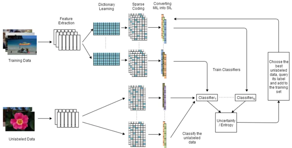
Recently, Song et al [27] proposed Sparse Coding and Classifier Ensemble based MIL method (SCCE-MIL) for image categorization. Their algorithm combines the ensemble strategy with sparse coding for the MIL framework. Overview of the SCCE-MIL algorithm can be shown in Figure 3.1. Essentially, their algorithm has 4 steps. Firstly, ensemble system is constructed by learning different sized dictionaries with the training data. Since dictionaries are trained with different sizes, they capture different structures of the signal. This aspect would yield diverse ensemble system that boost the overall classifier accuracy.
In order to train a dictionary in a MIL setting, we have to concatenate all the instances in the bags into an instance matrix. So, the resulting dictionary modals the instances of the bags. After the dictionary training, each instance in the bags is transformed into multiple sparse feature vectors using different sized dictionaries. While these sparse features represent the key elements in their own signal, they give higher level information about the data sample i.e. patterns in the signal. Also using sparse coding techniques removes the noises from the signal so that we can use sparse features instead of original features [28].
As we reviewed in Chapter 2.1, there are three approaches to solve a MIL problem. In SCCE-MIL algorithm, sparse representations for each instance is obtained. Using these representations, a single bag representation using max-pooling function is computed. Max pooling function allows us to convert the bag instances into a bag feature so that it summarizes the most influential features in the bag. Since the instances in the bags are sparse, calculating the maximum value would give best
20
21
contribution of the atom in the dictionary. This aspect of the max proven to be true for applications e.g. image categorization [29].
As the last step of SCCE-MIL algorithm, Support Vector Machines (SVM) is trained to learn the bag representations. Since SCCE-MIL is an ensemble algorithm multiple SVMs are trained on different sized bag features which are extracted from different sized dictionaries. Pseudo-code of the algorithm is given in Table 3.1.
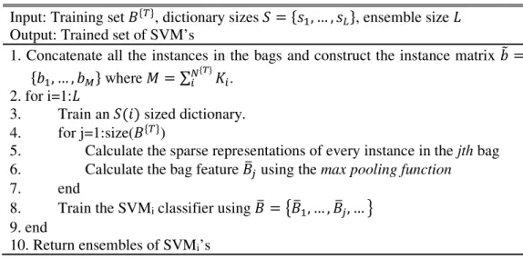
Table 3.1 :SCCE-MIL algorithm.
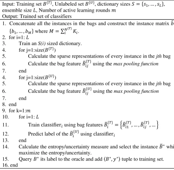
Input: Training set +{ƒ}, dictionary sizes • = {t., … , t_}, ensemble size b Output: Trained set of SVM’s
1. Concatenate all the instances in the bags and construct the instance matrix h =
{ ., … , i} where P = ∑j{k}5. 2. for i=1:b
3. Train an • • sized dictionary. 4. for j=1:size(+{ƒ})
5. Calculate the sparse representations of every instance in the jth bag 6. Calculate the bag feature +[ using the max pooling function 7. end
8. Train the SVMi classifier using +[ = -+[., … , +[ , … 3 9. end
10. Return ensembles of SVMi’s
After the training step, the test data is processed like the training data but, dictionary learning and SVM training steps are omitted. The trained dictionaries are used to obtain sparse coding of the test instances and trained SVM’s are used for classification. Once the results of the each SVM is calculated, their class decisions are combined using majority voting and the final result would be the class label of the test data.
Song et al [27] also analyzed the effect of the dictionary size but they didn’t consider the best ensemble size and the base classifier. In the next sections, experiments are carried to investigate those issues.
3.2Experimental Setup
Experiments are conducted on Corel 1000, 2000 [11], Elephant, Fox and Tiger [6] datasets. Corel 1000 and 2000 datasets are image dataset containing 10 and 20 different categories respectively. In the dataset, each category has 100 images and each image is a 384×256 or 256×384 sized JPEG file. Images are divided into
non-22
overlapping blocks of size 4x4 pixels. For constructing the image features, three separate feature extraction methods are applied. The first method is to average the LUV color components of the blocks. Secondly, wavelet transform is applied and squire root of energy values in the high frequency band is used. Lastly, the shape properties are calculated for each region. Once the feature extractions are made, all of the properties are aggregated as a one feature vector. The resulting feature vector for Corel 1000 and 2000 dataset is a 9-dimensional feature vector. In our experiments we used the calculated image features from [11]. Some example images in the Corel 1000 dataset are shown in Figure 3.2.
Figure 3.2 :Example images of COREL 1000 dataset [11].
Elephant, Fox and Tiger datasets are three image datasets where each of them contains 100 of animal images and 100 of other images in total of 200 images. All
23
images are separated into regions and each region is represented as a 320-dimensional feature vector which describes the color, texture and shape property of its region. For Elephant, Fox and Tiger datasets, we used the extracted image features from [6] directly.
For each dataset, we conducted the experiments 10-fold cross validation and average results are reported. For dictionary learning and sparse coding, SPAMS toolbox [26] is used. In SPAMS, we used LARS algorithm for sparse coding and Online Dictionary Learning for dictionary learning. In SCCE-MIL algorithm, Song et al. conducted their tests with SVM as the base classifier. We extended their research with different base classifier - Decision Tree (DT), Multi-Layer Perceptron (MLP) - and compare their performances. We also analyzed the ensemble size of the SCCE-MIL method. The implementation of the SVM is done with LIBSVM toolbox and the parameters are selected using grid search and best parameters are used. For MLP and DT, MATLAB toolbox is used.
3.3Experimental Results
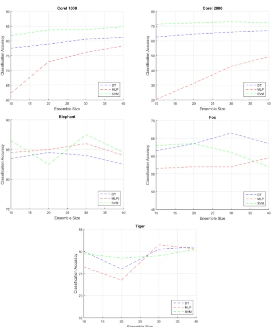
Classification accuracies with respect to the ensemble size of the SCCE-MIL algorithm are shown in Figure 3.3. As it can be seen from the figure, in Corel 1000, Corel 2000 and Elephant datasets, SVM gives the highest classification accuracy over DT and MLP. In Song et al. [27] work, they used Corel 1000 and 2000 for their experiments and their results are consistent with our experiments. But for Fox dataset, SVM performs poorly for large numbers of classifiers comparing with DT and MLP. For Tiger dataset all of the algorithms converge to the same accuracy level when the ensemble size is 40. Besides, in Fox dataset, DT performs significantly better than the other base classifiers when the ensemble size is 40. So the structure of the SCCE-MIL algorithm is powerful for image categorization but we need to test the base classifier according to the dataset.
When we increase the ensemble size of the system, classification accuracy increases for some dataset. For example, if we look for Corel 1000 and 2000 datasets, we can see the improvement of the accuracies. But, this result doesn’t apply to the other datasets. For example, in Elephant and Tiger datasets, all the algorithms deviate in terms of accuracy. In Fox dataset, SVM performance drastically decreases. The best performance can be achieved by DT for Fox dataset. Note that in SCCE-MIL
24
algorithm, authors constructed the classifier ensembles in an arbitrarily selected size, 40. As we can see from the figures, the best accuracies are generally achieved with the ensemble size 30.
Figure 3.3 :Result of the SCCE-MIL algorithm with different ensemble size and base classifier.
With these experiments, we investigate the issues regarding to the ensemble size and the base classifier selection. Our findings show that the best classifier and the ensemble size for the SCCE-MIL algorithm is a relative issue to the database which we try to model. In order to narrow down those issues for real applications, one needs to use a validation test to try to optimize the base classification and ensemble size.
25
4. DICTIONARY ENSEMBLE BASED MULTIPLE INSTANCE ACTIVE LEARNING
After the explanation of the SCCE-MIL algorithm, now we propose our Dictionary Ensemble Based Multiple Instance Active Learning algorithm, namely DEMIAL. Firstly, we will explain active learning and some strategies in the literature. Later, we will discuss our approach and present the results.
4.1Active Learning
In many real world machine learning problems, we encounter with few labeled data samples and abundant sized unlabeled data. Instead of modeling the data only with the labeled ones, one may try to include the unlabeled data. But this can be an enormous work to accomplish. Another approach would be that instead of labeling all the unlabeled data, we may choose some of the instances wisely and label them only. This technique is called active learning and it is widely used in many machine learning problems. The intuition is that active learner has the opportunity to select the unlabeled data so that learner yields better results with less data. This allows us to build classifiers with a dataset in which labeling is very expensive, difficult or time-consuming. In active learning terminology, labeling process is stated as querying the data label to an oracle (human or computer expert).
In active learning framework, the most important function is to find the most informative data sample in an unlabeled dataset. We need the informative data sample because it contributes to the classifier the most. Thus with the query function, active learning allows us to train better classifiers with fewer data samples.
Among the query strategies in the literature, the simplest and most used one is called
uncertainty sampling [30]. In uncertainty strategy, we choose the unlabeled data
which the classifier is the least certain about its label. If we think of a probabilistic classifier model for a binary classification problem, the unlabeled data sample having 0.5 posterior probability is selected and queried for its label [31]. As for non-probabilistic case, the data sample that is close to the decision boundary is queried.
26
Uncertainty can be measured using the following formula:
+∗= argmax
K2∈K{Ž}, `.…j{Ž}
1 − •• 4|+ (4.1)
where •• 4|+ is the posterior probability under the model ‘ and +∗ is the queried data sample.
This strategy is quite straightforward and intuitive but it only examines the most probable class information. This is not a problem for a binary classification problem, but for multi-class problem it may mislead. In particular, it doesn’t consider the other classes’ probabilities. To fix this problem, Scheffer et al. [32] proposed margin
sampling:
+∗= argmin
K2∈K{Ž}, `.…j{Ž}
•• 4.|+ − •• 4/|+ (4.2)
where 4. and 4/ is the most probable two classes under the model ‘. As we can see, margin sampling selects the minimum margin between class posterior probabilities. Querying the small margin gives the most ambiguous data sample between the two classes. But if we need the most ambiguous data sample among the dataset, margin sampling doesn’t necessarily gives it because it discards other classes’ informations. So as a more general strategy, uncertainty query should calculate the entropy of the posterior probabilities which can be shown as:
+∗= argmax
K2∈K{Ž}, `.…j{Ž}
− V ••„4 |+ … log ••„4 |+ … a
`. (4.3)
where ” is the number of class labels in the dataset.
Note that for binary classification problems this entropy-based query strategy will yield to the same result with margin and uncertainty strategies. But the entropy based approach generalizes easily to probabilistic multi-label classifiers [31].
4.2Multiple Instance Active Learning
In a single instance learning problem, active learning strategies are developed over the years but for MIL framework, it is not straightforward to apply these strategies. Because, the datasets are constructed as bag of instances so querying becomes a
27
confusing task. To address this problem, Settles et al [33] proposed the first Multiple Instance Active Learning strategy where they query the some of the instances in a selected bag. This would allow us to label just one instance instead of a whole bag of instances.
Their approach is useful for some applications where the instance labeling can be done. But for some applications, labeling an instance is not an easy task for human experts. To solve this problem, Fu et al. [34] adopted Fischer Information Matrix based query strategy for bag-level active learning. In their work, Fisher Information Matrix is constructed for the bags and the query is done by selecting the smallest fisher score.
Alternatively, to address this problem Liu et al. [35] proposed a kernel-based MI active learning. In their work, they used set kernels to calculate the distance between two bags. After the set kernel values are calculated, they trained an SVM classifier. As for the active learning, they proposed an MI Informativeness measure. In the informativeness measure, they combined three different metrics which utilize the kernel values of the bags. Those metrics are uncertainty, novelty and diversity measures. Uncertainty is the same measure that has given in equation 4.1 but in Liu et al. work, they used SVM classifier so instead of posterior probability, they used the objective function of SVM. So the uncertainty measure of a given data sample would be as the following:
• –+{—}˜ = 1 − ™V š 5YSTU–+{—}, +{ƒ}˜ j{k}
+ ™ (4.4)
where š is the Lagrangian multiplier of the support vectors.
The second metric for informativeness measure is the novelty measure. Intuition of the novelty measure is that unlabeled data sample which is close to the training data will be less likely to be queried. In this case, unlabeled data sample which is far away from the training data will have a higher chance to be selected. This approach allows us to improve our classifier model by selecting data sample with minimum overlapping with the training data. Novelty measure of an unlabeled data +{—} can be given as,
28
^ –+{—}˜ = 1 − max.œ œj{k}5YSTU–+{—}, +{ƒ}˜ (4.5)
Lastly, the third metric is the diversity measure. This measure calculates the diversity of a given unlabeled data sample between the whole unlabeled dataset. This metric prevents the query possibility of two almost the same unlabeled data samples. Diversity measure can be given as:
• –+{—}˜ = 1 − V 5YSTU–+{—}, +{—}˜ „žŸ {—}− 1… j{Ž}
`., Š
(4.6)
So far, we measured the proximity with the decision boundary with uncertainty measure, the diversity between training and unlabeled data sample with novelty measure and diversity among the unlabeled data with diversity measure. The combination of these three measurements would yield the MI Informativeness measurement which is given as follows:
P _ o¢£•q¤u•¥¦o¦tt –+{—}˜
= § × • –+{—}˜ + 1 − § × • –+{—}˜ × ^ –+{—}˜ (4.7)
where § is a trade-off parameter between metrics. After calculating the informativeness measure for every unlabeled data sample, unlabeled data sample which gives the maximum value is queried and added to the training data.
4.3Dictionary Ensemble Based Multiple Instance Active Learning
As stated in the previous section, there are some studies on combining the active learning techniques and MIL framework but these algorithms don’t benefit the advantages of sparse coding and classifier ensembles. So, we propose an MI active learning technique that uses sparse coding and classifier ensemble methods – as we call it DEMIAL. Overview of the proposed algorithm is shown in Figure 4.1. The DEMIAL algorithm combines SCCE-MIL and active learning and extends it by using different base classifiers and different active learning query strategies.
29

![Figure 3.2 : Example images of COREL 1000 dataset [11].](https://thumb-us.123doks.com/thumbv2/123dok_us/8996650.2797496/50.918.140.721.378.973/figure-example-images-corel-dataset.webp)