Analysis of interval-censored recurrent event processes subject to resolution

Analysis of interval-censored recurrent event processes

subject to resolution

HUA SHEN

Department of Statistics and Actuarial Science

,

RICHARD J COOK

Department of Statistics and Actuarial Science, University of Waterloo, Waterloo, ON, N2L 3G1, Canada

E-mail: [email protected]

Summary

Interval-censored recurrent event data arise when the event of interest is not readily observed but the cumulative event count can be recorded at periodic assessment times. In some settings, chronic disease processes may resolve, and individuals will cease to be at risk of events at the time of disease resolution. We develop an expectation-maximization algorithm for fitting a dy-namic mover-stayer model to interval-censored recurrent event data under a Markov model with a piecewise-constant baseline rate function given a latent process. The model is motivated by set-tings in which the event times and the resolution time of the disease process are unobserved. The likelihood and algorithm are shown to yield estimators with small empirical bias in simulation studies. Data are analysed on the cumulative number of damaged joints in patients with psoriatic arthritis where individuals experience disease remission.

Keywords: EM algorithm; Interval censoring; Mover-stayer model; Piecewise-constant rate func-tion; Recurrent events

This is the peer reviewed version of the following article: Shen, H. and Cook, R. J. (2015), Analysis of interval-censored recurrent event processes subject to resolution. Biom. J., 57: 725-742. doi: 10.1002/bimj.201400162, which has been published in final form at

http://dx.doi.org/10.1002/bimj.201400162. This article may be used for non-commercial purposes in accordance with Wiley Terms and Conditions for Self-Archiving:

http://olabout.wiley.com/WileyCDA/Section/id-820227.html#terms.

1

I

1.1 LITERATURE REVIEW AND GENERAL MOTIVATION

There are many chronic diseases for which affected individuals experience recurrent adverse events. Often it is apparent when the events occur, as is the case in respiratory disease when individuals experience exacerbations of symptoms (Grossman et al., 1998), neurologic disease where the events may be epileptic seizures (Pledger et al., 1994), migraine where the events are headaches (Pascual et al., 2000), and cardiology where the events may be acute angina attacks (Peters et al., 2003).

Statistical methods for recurrent event analysis in such settings include those reliant on intensity-based models (Andersen et al., 1993), random effect models (Lawless, 1987), and marginal methods (Lawless and Nadeau, 1995, Lin et al., 2000). Cook and Lawless (2007) give an account of the various frameworks for analysis.

The occurrence of an event is not evident in settings where they are not immediately symptomatic, but often they can be determined to have occurred at a subsequent clinic visit, radiographic exami-nation, or blood test. Examples of such events include the development of new superficial tumours in bladder cancer patients (Byar et al., 1986), the occurrence of asymptomatic fractures in patients with osteoporosis (Riggs et al., 1981), or the development of new skeletal metastases in patients with cancer metastatic to bone (Hortobagyi et al., 1996). A considerable amount of statistical research has taken place in recent years on the analysis of this type of data which is referred to as panel count data, grouped recurrent event data, or interval-censored recurrent event data. Two-sample tests were devel-oped by a number of authors including Thall and Lachin (1988), Sun and Fang (2003), Zhang (2006), Park et al. (2007) and Balakrishnan and Zhao (2009). Mean function estimation was considered by Sun and Kalbfleisch (1995), and their estimator was later shown by Wellner and Zhang (2000) to be a pseudo-maximum likelihood estimator under a nonhomogeneous Poisson model; these authors proved consistency, along with their proposed maximum likelihood estimator which did not depend on the Poisson assumption. Sun and Wei (2000), Cheng and Wei (2000), Zhang (2002) and Wellner and Zhang (2007) developed methods for semiparametric regression with interval-censored recurrent event data. Lawless and Zhan (1998) consider multiplicative recurrent event models with piecewise-constant baseline rate functions fitted via estimating functions as well as fully specified random effect models fitted using maximum likelihood. Such piecewise-constant models share the advantages of parametric models and yet provide some robustness to misspecification of the parametric form of rate functions. Chen et al. (2005) extend these methods to deal with multi-type recurrent events. Sun and Zhao (2013) give an excellent account of the recent developments on methods for recurrent event analysis when data are subject to interval-censoring.

In some settings the chronic condition generating the events can resolve and from the point of resolution individuals will no longer be at risk of events. Establishment of suitable medications, removal of stressors in mental health studies (Kessing et al., 2004), or other lifestyle changes may minimize risk of future events, but it can be difficult to determine if and when such changes have taken place. In other settings, the disease process resolves naturally. Polymyalgia rheumatica (Salvarani et al., 2002), for example, is an autoimmune disease and in the most active phase patients experience recurrent acute episodes of pain in the shoulder and pelvic joints. This active phase is of variable length but upon completion the acute episodes cease to arise (Healey, 1984). Patients with systemic lupus erythematosus experience flares of lupus nephritis, but this condition can go into remission such that patients stop experiencing acute flares (Barber et al., 2006). The disease in many rheumatological conditions can go into remission (Gladman et al., 2001, Zochling and Braun, 2006). In these and other settings one is faced with the challenge of interval-censored recurrent event times with the need to accommodate the possibility that the underlying condition has resolved. In the next sub-section, we describe a registry of patients with psoriatic arthritis and the scientific objectives of the associated research program which motivated the developments in this paper.

1.2 DIEASE PROGRESSION AND THE UNIVERSITY OF TORONTO PSORIATIC ARTHRITIS CO

-HORT

Psoriatic arthritis is an inflammatory arthritis and an autoimmune disease that commonly occurs among patients with psoriasis. Patients with psoriatic arthritis may experience swelling, pain and inflammation in the affected joints. The University of Toronto Psoriatic Arthritis Clinic is the largest center in the world for specialized care and research in this disease. The clinic, started in 1978, has been recruiting and following patients continuously since then. Data collected at clinic entry and

reg-ular follow-up clinic visits arise from a complete history, physical examination, blood and urine tests, and radiographic examination. Over 1100 patients have been closely followed over the years.

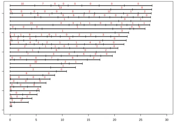
The development of joint damage is of primary interest to clinicians since this damage impairs functional ability and quality of life. Much of the scientific research on this condition is directed at understanding the risks of rapid onset and accumulation of damage (Gladman et al., 1995). Factors studied include information on family history of psoriatic arthritis and genetic information based on human leukocyte antigen (HLA) markers, for example. Radiological examinations of the hands, feet and spine are scheduled every two years, but the actual assessment times vary considerably. Moreover, there are some patients who experience no joint damage over the entire course of follow-up, and others who develop damaged joints for some time but then have long periods of time in which no further damage is observed. One possible explanation for the latter scenario is that these patients experience remission and hence are no longer at risk for further damage. A key point is that individuals may transition from the mover (susceptible to damage) to stayer (remission) subgroup as time passes. Figure 1 displays the timing of the assessments (hatch marks) and the number of additional damaged joints detected (red numbers) over the respective intervals for a sample of 27 individuals; here we restrict attention to patient data over the first 30 years from disease onset. The variability in the frequency of visits is apparent, as is the variation in the event counts between patients and within patients overtime. 0 5 10 15 20 25 30 0 5 10 15 20 25

YEARS SINCE ONSET OF PSA

ID l l0 l2l 0 l l l0 0 l 0 l l 0 l 0 l l l l l 0 0 0 l0l 0 l 0 l l 0 l 0 l 0 l ll l l l 0l 0 0 l0 l 8 0 l 2 l 0 l l 0 l 1 l l 32 l 2 l 1 l l0l 0 l 0 l 7 l 9 l 2 l l 7 l 3 l 6 l 6 l 0 l 0 l l 0 l 1 l 8 l 0 l 2 l l 2 l 1 l 1 l 0 l 0 l 2 l 0 l ll l l l l l l l l l 6l l 1 l 4 l1 2 1 1 4 3 l 0 l 2 1 0 3 0 ll l l l l l l l l l l l 0l 1 1 9 1 0 1 0 2 2 3 l 1 l 1 3 l0l 0 l 0 l 1 l 0 l0l 0 l l 21 l 3 l 3 l 1 l 1 l 0 l 0 l 1 l 1 l 1 l l 1 l 0 l 1 l l 8 l 4 l 7 l 9 l 9 l 1 l 2 l 0 l 0 l 0 l 0 l 0 l l l0 0 l 0 l 0 l 0 l 0 l 2 l 11 l 1 l 2 l l 13 l 3 l 6 l l 10 l 7 l 0 l 0 l 0 l 0 l 0 l 0 l

Figure 1: Plot of assessment times (hatch marks) and the number of damaged joints determined to have arisen between assessments (red numbers) by radiological examination for a selected sample of patients in the University of Toronto Psoriatic Arthritis Clinic; follow-up is restricted to the first 30 years following disease onset

HLA-B27 (human leukocyte antigen B27) is a protein found on the surface of white blood cell that has been found to be strongly associated with inflammatory autoimmune diseases such as ankylosing

spondylitis and psoriatic arthritis. Interest here lies in examining the effect of this HLA marker on the occurrence of damage as determined by radiographic examination of patients with psoriatic arthritis. When radiographs are taken, the extent of damage is assessed in each of 42 joints, including 30 hand joints (wrists, metacarpophalangeals, proximal interphalangeals and distal interphalangeals) and 12 joints in the foot (metatarsophalangeals and interphalangeal fist toes). The extent of damage in each joint is recorded on a six-point scale with numeric scores of 0 (normal), 1 (soft tissue swelling), 2 (surface erosions), 3 (joint space narrowing), 4 (disorganization, including subluxation, pencil-in-cup deformity and ankylosis), or 5 (damaged to the point of requiring surgery). A joint scoring 2 or higher is counted to be damaged to the point of impacting functional ability so the numbers in Figure 1 reflect the number of joints with at least grade 2 damage. Following the development of the proposed model and the algorithm for estimation, we return to this study in Section 3.2.

The remainder of this paper is organized as follows. In Section 2.1, the dynamic mover-stayer model is formulated. The complete data likelihood is constructed for the setting with interval-censored event times in Section 2.2 for a conditional Markov process for event occurence, and the requisite conditional expectations are derived in Section 2.3; details on how to implement the EM algorithm are given in the Appendix. The performance of the proposed model and algorithm are eval-uated empirically in Section 3.1 and data from a psoriatic arthritis cohort are analysed in Section 3.2. General remarks and areas of further research are given in Section 4.

2

A

-

-

2.1 FORMULATION OF THE DYNAMIC MOVER-STAYER MODEL

Shen and Cook (2014) recently proposed a dynamic mover-stayer model for the analysis of right-censored recurrent event data that accommodates unusually long times from the last observed event to the right censoring time. If T0 = 0 denotes the time of an initiating event such as the onset of a chronic disease, then Tj represents the time of thej-th subsequent event, j = 1,2, . . .. If N(t) =

P∞

j=1I(Tj ≤ t)denotes the number of events over(0, t], then{N(s),0 ≤ s}is a counting process.

The possible resolution of the process is accommodated by the introduction ofZj, a time-dependent

indicator, such that Zj = 1 if the individual remains at risk of events following the occurrence of

thejth event, andZj = 0otherwise,j = 0,1, . . .. The resolution of the chronic condition upon the

j-th event is reflected by a realizationZj = 0whenZj−1 = 1. Figure 2 is a schematic relating the random event times and random mover-stayer indicators for a hypothetical individual experiencing six events before resolution of the condition atT6; the dashed line followingT6 relects the fact that this individual is no longer at risk of events. In generalZj is a latent variable, but it is apparent that

Zj = 1 as soon as the (j + 1)-st event occurs, j = 0,1, . . .. As a consequence when events are

observed in continuous time (or subject to right-censoring) the only unknown mover-stayer indicator is the one corresponding to the last observed event.

We letXdenote a fixed covariate vector containing information on the characteristics of each indi-vidual observed upon recruitment to a cohort. We letZ¯(t) ={Z0, . . . , ZN(t)}denote the history of the mover-stayer indicators for all events arising over[0, t]andZ¯j ={Z0, . . . , Zj}denote the analogous

history when viewed as a function of the event count. The complete process history is then denoted byH(t) ={N(s),0≤s≤t,Z¯(t), x}, which includes the values of the latent variables realized over

[0, t], and the history excluding the partially latentZ¯(t)is denoted byH(t) ={N(s),0≤s ≤t, x}. We let t− denote an infinitesimal amount of time before t, N(s, t) = N(t−)−N(s−) denote the number of the events over[s, t), and∆N(t) =N(t, t+ ∆t)denote the number of the events over the interval[t, t+ ∆t). Thecomplete data intensity functionis then

λ(t|H(t−)) = lim ∆t↓0 P(∆N(t) = 1|H(t−)) ∆t =ZN(t−)λ(t|H(t −_)), (1)

| | | | | | | | T0=0 T1 T2 T3 T4 T5 T6 τ

Z0=1 Z1=1 Z2=1 Z3=1 Z4=1 Z5=1 Z6=0

TIME SINCE DISEASE ONSET, t − − − − − − − − 1 2 3 4 5 6 7 CUMULA

TIVE NUMBER OF EVENTS

, N(t)

Figure 2: Schematic relating the observed and latent random variables in the dynamic mover-stayer model for a hypothetical individual experiencing six events before resolution atT6

and thecanonical event intensity functionis

λ(t|H(t−)) = lim

4t↓0

P(4N(t) = 1|H(t−))

4t . (2)

Theintensity functionfor the observable process (in the absence of censoring) is given by

E{λ(t|H(t−))|H(t−)}=E(ZN(t−₎|H(t−))·λ(t|H(t−)).

The probability of remaining at risk following thej-th event can depend uponH(t−_j), so attj we

write this as

P(Zj = 1|H(t−j ), dN(tj) = 1) =P(Zj = 1|H(t−j),Z¯j−1 = 1j−1, dN(tj) = 1), (3)

wheredN(t) = lim∆t↓0∆N(t)indicates whether an event occurred at timetand1j−1is aj×1vector of ones. This probability may therefore depend on the times of previous events and the history of the observable covariates over[0, tj]and is only relevant ifZ¯j−1 = 1j−1. Herej = 0,1, . . ., H(t−0) = ∅ andZ¯−1 =∅.

2.2 THE COMPLETE DATA LIKELIHOOD FOR INTERVAL-CENSORED DATA

We now consider the setting in which individuals are only seen intermittently but continue to fo-cus on the contributions from a single individual. While the general formulation of the model in the previous section can be exploited for right-censored data, as in most settings involving interval-censored life history processes (Kalbfleisch and Lawless, 1985), we focus here on processes which are Markov given the mover-stayer indicators. We let a0 = 0 denote the time of a baseline as-sessment at which a fixed covariate vector x is observed, and let a1 < · · · < aR denote the times

of the follow-up assessments. At the r-th follow-up assessment at time ar, the number of events

over interval Ar = [ar−1, ar) is recorded and we denote this more compactly at times by nr =

N(ar−1, ar), r = 1, . . . , R, where n =

PR

denoted byHr = {(a`, n`), `= 1,2, . . . , r, x}. The full data for an individual is then D = HR =

{(ar, nr), r= 1, . . . , R, x}.

We assume individuals are observed from the time of disease onset in which case N(0) = 0and H0 simply contains the covariate data. In the present setting, this is reasonable because individuals invariably seek medical care when joints become inflamed, which occurs considerably earlier to the development of joint damage. Since the times of the assessments are random, the observed data likelihood is L∝ R Y r=1 P(Nr =nr, Ar =ar|Hr−1).

The assessment process is sequentially ignorable (Hogan et al., 2004, Lawless, 2013) in a likelihood based analysis if given Hr−1, the probability an assessment is made at ar is independent of event

occurence over[ar−1, ar). Under this assumption (i.e.Ar⊥N(ar−1, ar)|Hr−1), we can write

P(Nr, Ar =ar|Hr−1) = P(Nr|Ar =ar, Hr−1)P(Ar =ar|Hr−1),

(Cook and Lawless, 2014). Furthermore, if the inspection process is non-informative, we can disre-gard the contributions of the formP(Ar =ar|Hr−1)and work with the resulting partial log-likelihood

logL=

R

X

r=1

logP(Nr =nr|Ar =ar, Hr−1) (4)

without any loss of efficiency. Maximization of (4) is challenging however, since the expression for the necessary conditional probabilities are complicated and existing software cannot be used for maximization of this objective function. We develop an expectation-maximization algorithm in what follows.

Let θ1 index the canonical event intensity (2), θ2 index the mover-stayer model (3), and θ =

(θ₁0, θ₂0)0. A complete data log-likelihood corresponding to (4) can be constructed by considering the event times and the latent mover-stayer indicators as observed. The contribution to such a log-likelihood from an individual is then

`C(θ) =`C1(θ1) +`C2(θ2) (5) where `C1(θ1) = Z ∞ 0 Y(u)

dN(u) logλ(u|H(u−))−ZN(u)λ(u|H(u−))du

(6) `C2(θ2) = n X j=0 logP(Zj|H(t−j),Z¯j−1 = 1j−1, dN(tj) = 1) (7)

pertain to the event process and mover-stayer model, respectively, andY(u) = I(u≤aR).

Suppose interest lies in modeling data from individuals over the interval [0, τ] whereτ is fixed. We focus here on settings with latent multiplicative Poisson processes, whereλ(t|H(t−)) =ρ(t|x) = ρ0(t) exp(x0β)andρ0(t) is the canonical baseline rate function. Given a set of cut-points0 = b0 < b1 < · · · < bK = τ, a piecewise-constant baseline rate function is obtained by letting ρ0(t) = ρk

for t ∈ Bk = [bk−1, bk), k = 1, . . . , K. Let ujk = I(j = k), j = 1,2, . . . , K, k = 1,2, . . . , K,

xk = (u1k, . . . , uKk, x0)0, uk(t) = I(t ∈ Bk), k = 1,2, . . . , K, and x(t) = (u1(t), . . . , uK(t), x0)0.

One can then write

ρ(t|x;θ1) =ρ0(t;α) exp(x0β) = exp(x0(t)θ1) =

K

Y

k=1

− − − a0 a1 a2 a3 | | | | b0 b1 b2 b3 b4 n1=2 n2=3 n3=1 Observed Counts Baseline Intensity ρ1 ρ2 ρ3 ρ4

Individuals Assessment Times and Counts

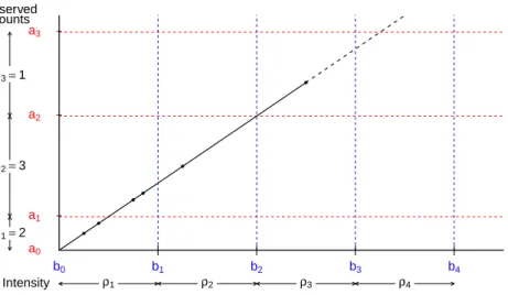
Figure 3: A two-way plot of the cut-points (horizontal axis), assessment times (vertical axis) and events (dots on the diagonal timeline); this hypothetical individual experienced six events before disease resolution atT6

where αk = logρk, k = 1, . . . , K, α = (α1, . . . , αK)0 and θ1 = (α0, β0)0. Figure 3 illustrates the observed counts and time intervals using this notation for a hypothetical individual experiencing six events before disease resolution atT6.

We let Crk =Ar ∩ Bk = [Cr,k−1, Crk)and letKr ={k :Ar∩ Bk 6= ∅}represent the labels for

theqr (0 < qr ≤ K) pieces intersecting Ar, denoted{k`r, ` = 1, . . . , qr}. If we letnrk =

R

I(u ∈

Crk)dN(u)denote the number of events overCrkandwk(t) =

Rt

0 I(u∈ Bk)dudenote the time at risk inBkover(0, t], then (6) can be rewritten as

K X k=1 n_XR r=1 nrk(αk+x0β)−[Znwk(aR) + (1−Zn)wk(tn)] exp(αk+x0β) o . (8)

There are many discrete waiting time models suitable for modeling the resolution of the process. The model in (3) suggests that the conditional probability that the process resolves attj can depend

on the history up to t−_j , but this is of course not observed under an intermittent inspection process. While such dependence could be handled by treating this as a missing covariate problem we assume instead that

P(Zj = 1|H(t−j),Z¯j−1 = 1j−1, dN(tj) = 1) =P(Zj = 1|x,Z¯j−1 = 1j−1) in which case we may adopt a logistic model of the form

logitP(Zj = 1|H(t−j ), dN(tj) = 1) = ˙xj0γj (9)

wherex˙j = (1, j, x0)0.

2.3 DERIVATION OF THE CONDITIONAL EXPECTATIONS

Since the actual events times and the final mover-stayer indicator are not observed, the quantities nrk, wk(aR), wk(tn), and Zn in (8) are unknown and we require expressions for their conditional

expectations (Dempster et al., 1977). We focus initially on the expectations given D and Zn, and

consider first the case in whichZn = 1. We let

η_rk(1) =E(nrk|D, Zn = 1) =

nrµrk

P

k∈Krµrk

where

µrk =

Z

I(u∈ Crk)ρ(u|x)du= exp(αk+x0β)|Crk|,

and|Crk|denotes the length ofCrk,k ∈ Kr, r = 1, . . . , R(Lawless and Zhan, 1998). A superscript

of1is used in (10) to reflect the fact that the expectation is conditional onZn = 1. Sincewk(aR) =

PR

r=1wrk(aR)wherewrk(aR) =

RaR

0 I(u∈ Crk)du, givenZn= 1we can write ω_rk(1) =E(wrk(aR)|D, Zn= 1) =|Crk|.

Ifsdenotes the index for the inspection interval containingtn, the time of the final event observed

over(0, τ](i.e. tn ∈ As), then forr < s,E(nrk|D, Zn = 0) =E(nrk|D, Zn = 1)as in (10), and for

r > s,E(nrk|D, Zn = 0) = 0,k ∈ Kr, by the definition ofAs. Note thatE(nsk|D, Zn= 0),k ∈ Ks,

can be obtained by conceptualizing a progressive time nonhomogeneous multistate Markov process with a finite number of states labelled N(as−1), . . . , N(as) where only ` → `+ 1 transitions are

allowed with a common “transition” intensityρ(u|x),` =N(as−1), . . . , N(as)−1andN(as) =nis

an absorbing state. We letns = (nsk, k=k1s, . . . , ksqs)denote the counts over the subintervals ofAs,

letn¯sk = n(as−1) +

P

j∈KsI(j ≤k)nsj denote the cumulative count atCsk, and letn¯s = (¯nsk, k =

k₁s, . . . , ks_qs)denote the vector of cumulative counts. We can then writeP(ns|D, Zn= 0)as

P(N(Csk) = ¯nsk for allk ∈ Ks|N(as−1) = n(as−1), N(as) = n(as), x, Zn = 0),

wheren(as−1) =n−nsandn(as) =nby the definition ofAs. This can in turn be written as

P(ns|D, Zn= 0) =

P(N(Csk) = ¯nsk for allk ∈ Ks|N(as−1) = n(as−1), x, Zn= 0)

P(N(as) = n|N(as−1) = n(as−1), x, Zn= 0)

, (11)

where the numerator is equal to

Y

k∈Ks

P(N(Csk) = ¯nsk|N(Cs,k−1) = ¯ns,k−1, x, Zn = 0) (12)

by the Markov property, and the denominator is

X ns∈Ns Y k∈Ks P(N(Csk) = ¯nsk|N(Cs,k−1) = ¯ns,k−1, x, Zn = 0), (13) whereNs = {ns :ns = P

k∈Ksnsk}is the set of all vectorsnscompatible with observed total. To

determine the terms in (12), for a given vectornsconsider the specific subintervalCs` containingtn

(i.e.tn∈ Cs`). Fork∈ Kswithk < `, we have

P(N(Csk) = ¯nsk|N(Cs,k−1) = ¯ns,k−1, x, Zn = 0) =µnsksk exp(−µsk)/nsk!,

whereµsk = exp(αk+x0β)|Csk|, and whenk > `, P(N(Csk) = ¯nsk|N(Cs,k−1) = ¯ns,k−1, x, Zn =

0) = 1. Whenk =`, a time-homogeneous Markov process governors events overCs`with allowable

transitions0→1→ · · · →N` =ns`occurring with rateexp(α`+x0β).

Note that the probability of making transition from stateito statej, i, j = 0, . . . , N`, within time

tis

Pij(t) = (exp(α`+x0β)t)j−iexp(−exp(α`+x0β)t)/(j −i)! (14)

if0≤i≤j < N`, withPiN`(t) = 1−

PN`−1

j=i Pij(t)if0≤i≤ N`−1. Given this we can calculate

P(N(Cs`) = ¯ns`|N(Cs,`−1) = ¯ns,`−1, x, Zn = 0)as P0N`(|Cs`|). Also note that (11) can be used to

compute the conditional expectation for the counts in each subinterval ofAssince

η(0)_sk =E(nsk|D, Zn= 0) = ns

X

nsk=0

whereP(nsk|D, Zn= 0) =P_ns∈NsI(Nsk =nsk)P(ns|D, Zn= 0)for anyk∈ K s_.

Forr < s,E(wrk(tn)|D, Zn= 0) =|Crk|for allk ∈ Krand forr > s E(wrk(tn)|D, Zn= 0) = 0

for allk ∈ Kr _{by the definition ofA}

s. For r = s, Ks = {k`s, `= 1, . . . , qs}, and for a given vector

of counts ns = (nsk, k ∈ Ks), we can find an` such that tn ∈ Cs`. Once again, fork ∈ Ks, when

k < `, we haveE(wsk(tn)|D, Zn = 0) = |Csk|and whenk > `,E(wsk(tn)|D, Zn = 0) = 0by the

definition ofCs`. Whenr =s, andk =`,

ws`(tn) = Z tn 0 I(u∈ Cs`)du = Z Cs` I(tn> u)du = Z Cs` I(N(u)< n)du ,

and foru∈ Cs`, the latter expression can be helpful sinceP(N(u)< n|D, Zn = 0,ns)is ns`−1 X j=0 P(N(u) =j|N(Cs,`−1) = 0, x, Zn = 0)P(N(Cs`) =ns`|N(u) = j, x, Zn= 0) P(N(Cs`) =ns`|N(Cs,`−1) = 0, x, Zn = 0) . (16)

Note that over Cs`, we again have a continuous time Markov process with a time homogenous

transition intensity exp(α` +x0β) and transitions from ` to ` + 1 for ` = 0, . . . , N` − 1 where

N` =ns`, we can therefore use (14) to obtain the values of the three items in (16) for givenu ∈ Cs`,

and obtain

E(ws`(tn)|D,ns, Zn= 0) =

Z

Cs`

P(N(u)< n|D,ns, Zn = 0)du (17)

via numerical integration. Finally, for anyk ∈ Ks_,

E(wsk(tn)|D, Zn = 0) =

X

ns∈Ns

E(wsk(tn)|D,ns, Zn= 0)P(ns|D, Zn= 0),

whereP(ns|D, Zn = 0)is given in (11).

Let Hs = {(ar, nr), r= 1, . . . , s, x}denote the inspection times and counts up to and including

the inspection interval containing the last event known to have occurred, along with the covariate vector. The remainder of the data are denoted byHs+1,R ={(ar, nr), r =s+ 1, . . . , R, x}. Then

ζ = P(Zn = 1|D) = P(Zn = 1|D,Z¯n−1 = 1n−1) = P(Hs+1,R|Hs, Zn= 1, ¯ Zn−1 = 1n−1)P(Zn= 1|Hs,Z¯n−1 = 1n−1) P1 z=0P(Hs+1,R|Hs, Zn =z,Z¯n−1 = 1n−1)P(Zn =z|Hs,Z¯n−1 = 1n−1) (18) where P(Hs+1,R|Hs, Zn =z,Z¯n−1 = 1n−1) = R Y r=s+1 P((ar, nr)|Hr−1, Zn =z,Z¯n−1 = 1n−1).

Note thatP((ar, nr)|Hr−1, Zn=z,Z¯n−1 = 1n−1)can be written as

P(nr|ar, Hr−1, Zn=z,Z¯n−1 = 1n−1)P(ar|Hr−1, Zn =z,Z¯n−1 = 1n−1).

If ar⊥Zn|Hr−1,Z¯n−1 = 1n−1, under the conditionally (givenZn = z) sequentially missing at

ran-dom assumption (Hogan et al., 2004), the second term on the right-hand side does not depend onz. Moreover,

P(nr= 0|ar, Hr−1, Zn =z,Z¯n−1 = 1n−1) =

exp(−µr) ifz = 1

whereµr =

R

Arρ(u|x)du =

P

k∈Krµrk forr = s+ 1,· · · , R. Under the conditionally sequentially

MAR assumption,P(Zn=z|Hs,Z¯n−1 = 1n−1)is given by

P(ns|as, Hs−1, Zn =z,Z¯n−1 = 1n−1)P(Zn =z|Hs−1,Z¯n−1 = 1n−1)

P1

z=0P(ns|as, Hs−1, Zn=z,Z¯n−1 = 1n−1)P(Zn =z|Hs−1,Z¯n−1 = 1n−1) ,

whereP(Zn= 1|Hs−1,Z¯n−1 = 1n−1) =P(Zn= 1|x,Z¯n−1 = 1n−1)is given by (9) andP(ns|as, Hs−1, Zn=

0,Z¯n−1 = 1n−1)is given by (13).

3

E

S

A

3.1 DESIGN AND INTERPRETATION OF SIMULATION STUDIES

In this section, a simulation study is conducted to evaluate the performance of the method proposed to deal with interval-censored recurrent event data with disease resolution. We letXidenote a binary

covariate for individual i which takes on the value of 1 or 0 with equal probability to reflect, for example, whether an individual is on an experimental or control treatment. We then generate the initial mover-stayer indicatorsZij,j = 0,· · · , ni, following the model

logitP(Zij = 1|Xi,Z¯i,j−1 = 1j−1) =γ0+γ1j+γ2Xi ,

whereni is the total number of events observed over the entire study period(0, τ]if there is

admin-istrative censoring only. For simplicity, we set τ = 1 for all subjects. γ1 and γ2 are set aslog 0.95 andlog 0.75respectively, so that for given treatmentXi, the odds of being a mover decreases by 5%

with the occurrence of each additional event for the same treatment group, and the odds of being a mover is 25% lower if Xi = 1 compared to when Xi = 0 for a givenNi(t). For the purpose of

illustration, we assume the events are generated according to a homogenous Poisson process among movers, in which case the gap times follow an exponential distribution with rateλexp(Xiβ); hereλ

is the baseline intensity andβis reflects the treatment effect on the event rate. We setβ = log 0.75so that there is a 25% reduction in the event rate among movers on treatment and solve for λsuch that the expected number of events over(0, τ]is 6 or 12 among individuals for whom the disease process does not resolve. We then solve for γ0 to ensure the expected number of events over (0, τ] is 1.5, 3 or 6. A piecewise-constant baseline intensity model was adopted wherein cut-points were set by dividing the observation period(0, τ]evenly intoK = 3intervals.

For simplicity, we assume here that each subject has the same number of prescheduled evenly spaced assessments with Ri = R = 4 or 8; as described in Section 2 we observe only the

num-ber of events occuring between clinic visits, along with the treatment indicator. If ϑ = (α1, α2 − α1,· · · , αK−α1, β, γ0, γ1, γ2), we terminate the EM algorithm of the previous section whenmax(|ϑnewj −

ϑold_j |)< , where = 10−6. A total of 2000 simulations were conducted for each parameter

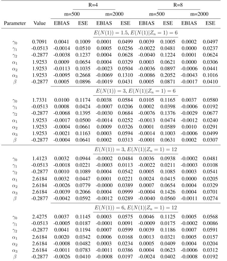
configu-ration with a sample size ofm= 500or2000. The empirical biases (EBIAS) and empirical standard errors (ESE) are reported in Table 1.

The simulation results in Table 1 show that the empirical biases are generally small, and decrease as the sample size increases. Moreover for a given sample size, the estimators have smaller empirical biases and smaller empirical standard errors the more frequent the assessments. When the expected numbers of events among the movers are the same, the covariate effects on the recurrent event pro-cess have smaller empirical biases and smaller empirical standard errors when the marginal expected number of events is larger; in such cases, the empirical standard errors in the estimates of the event rate are also smaller. For a given marginal expected numbers of events, both the association between the explanatory variables and the mover-stayer indicator and the covariate effect on the event process have smaller standard errors and negligible biases. When the assessment times are governed by a Poisson process, similar results are seen.

Table 1: Simulation results where the gap times follow an exponential distribution by adopting a piecewise-constant model when the data are subject to administrative censoring only, m = 500 or m= 2000,nsim= 2000,= 10−6

R=4 R=8

m=500 m=2000 m=500 m=2000

Parameter Value EBIAS ESE EBIAS ESE EBIAS ESE EBIAS ESE

E(N(1)) = 1.5,E(N(1)|Zn = 1) = 6 γ0 0.7091 0.0041 0.1009 0.0001 0.0499 0.0039 0.1005 0.0002 0.0497 γ1 -0.0513 -0.0014 0.0510 0.0005 0.0256 -0.0022 0.0481 0.0000 0.0237 γ2 -0.2877 -0.0038 0.1237 0.0004 0.0628 -0.0040 0.1224 0.0001 0.0624 α1 1.9253 0.0009 0.0654 0.0004 0.0329 0.0003 0.0621 0.0000 0.0306 α2 1.9253 -0.0113 0.1035 -0.0023 0.0504 -0.0036 0.0897 -0.0006 0.0441 α3 1.9253 -0.0095 0.2668 -0.0069 0.1310 -0.0086 0.2052 -0.0043 0.1016 β -0.2877 0.0005 0.0896 -0.0019 0.0431 0.0005 0.0871 -0.0017 0.0410 E(N(1)) = 3,E(N(1)|Zn = 1) = 6 γ0 1.7331 0.0100 0.1174 0.0038 0.0584 0.0105 0.1165 0.0037 0.0580 γ1 -0.0513 0.0008 0.0424 -0.0007 0.0206 0.0002 0.0398 -0.0006 0.0192 γ2 -0.2877 -0.0068 0.1395 -0.0030 0.0684 -0.0076 0.1376 -0.0029 0.0677 α1 1.9253 -0.0017 0.0500 -0.0014 0.0252 -0.0013 0.0474 -0.0012 0.0240 α2 1.9253 -0.0004 0.0661 0.0009 0.0326 0.0001 0.0589 0.0010 0.0291 α3 1.9253 -0.0021 0.1163 0.0003 0.0594 -0.0014 0.1003 -0.0006 0.0499 β -0.2877 -0.0004 0.0641 0.0002 0.0313 -0.0001 0.0631 0.0002 0.0307 E(N(1)) = 3,E(N(1)|Zn= 1) = 12 γ0 1.4123 0.0032 0.0944 -0.0002 0.0484 0.0036 0.0938 -0.0002 0.0481 γ1 -0.0513 -0.0018 0.0221 -0.0003 0.0113 -0.0022 0.0211 -0.0003 0.0108 γ2 -0.2877 0.0010 0.1089 0.0004 0.0542 0.0005 0.1085 0.0003 0.0541 α1 2.6184 0.0032 0.0447 0.0001 0.0221 0.0024 0.0415 0.0000 0.0205 α2 2.6184 -0.0026 0.0779 -0.0000 0.0389 0.0007 0.0654 0.0004 0.0329 α3 2.6184 -0.0039 0.2066 0.0004 0.0999 -0.0004 0.1426 0.0004 0.0701 β -0.2877 -0.0042 0.0592 -0.0012 0.0289 -0.0040 0.0560 -0.0011 0.0274 E(N(1)) = 6,E(N(1)|Zn= 1) = 12 γ0 2.4275 0.0037 0.1145 0.0003 0.0575 0.0046 0.1125 0.0005 0.0568 γ1 -0.0513 -0.0005 0.0187 -0.0001 0.0091 -0.0009 0.0175 -0.0002 0.0086 γ2 -0.2877 0.0041 0.1194 0.0007 0.0599 0.0039 0.1186 0.0007 0.0591 α1 2.6184 0.0020 0.0342 0.0006 0.0168 0.0013 0.0321 0.0005 0.0157 α2 2.6184 -0.0008 0.0482 0.0003 0.0234 0.0005 0.0409 0.0004 0.0204 α3 2.6184 -0.0011 0.0783 -0.0011 0.0386 0.0004 0.0623 -0.0006 0.0312 β -0.2877 -0.0026 0.0410 -0.0008 0.0197 -0.0024 0.0402 -0.0008 0.0192

3.2 APPLICATION TO JOINT DAMAGE IN PSORIATIC ARTHRITIS

We consider a subcohort of patients with psoriatic arthritics from University of Toronto Psoriatic Arthritis Clinic. These 207 selected patients have disease onset time and HLA-B27 information available. They entered the clinic and were followed-up between 1978 and 2013. The observation period is limited to the first 30 years following disease onset. The reported age of disease onset is taken as the time origin and dates of radiological assessments and numbers of new damaged joints were recorded at the following assessment visits. The average time since disease onset to first radio-logical assessment is 5.54 years (S.D. 6.02, range 0.03 to 27.23). The average number of radioradio-logical assessments within 30 years of disease onset is 3.63 (S.D. 2.83, range 1 to 13). A total of 32 (15.5%) patients are HLA-B27 positive.

The data suggested that some patients experience remission during the follow-up. We fit the proposed algorithm on the interval-censored recurrent event data to study the occurrence of joint damage. Piecewise-constant baseline rate functions are adopted to model the recurrent event process not subject to resolution with one fixed covariate HLA-B27 (X = 1if HLA-B27 positive, X = 0 if HLA-B27 negative); The canonical baseline rate are assumed to be constant for every 10 years. A dynamic mover-stayer model is fitted with the cumulative number of damaged joints (j) and HLA-B27 (X) being the explanatory variables in the logistic regression. A recurrent event model treating all patients as susceptible for joint damage is fitted for comparison, in which a piecewise-constant baseline rate model is assumed as well and the effect of HLA-B27 on event rate is also of interest.

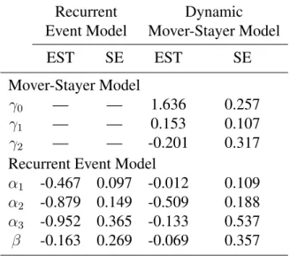
The estimation results, presented in Table 2, demonstrate that the event rate is noticeably under-estimated when all the patients are assumed to experience joint damage over the entire observation period. The effect of HLA-B27 on event rate is also underestimated though it is not significant in either model. The increased number of damaged joints is associated with higher odds of continuing to have new damaged joints.

Table 2: Results of fitting piecewise-constant baseline rate model and dynamic mover-stayer model to study the occurrence of joint damage among patients with psoriatic arthritis whose follow-ups are within 30 years of disease onset;m= 207, standard errors based on 100 bootstrap samples

Recurrent Dynamic

Event Model Mover-Stayer Model

EST SE EST SE

Mover-Stayer Model

γ0 — — 1.636 0.257

γ1 — — 0.153 0.107

γ2 — — -0.201 0.317

Recurrent Event Model

α1 -0.467 0.097 -0.012 0.109

α2 -0.879 0.149 -0.509 0.188

α3 -0.952 0.365 -0.133 0.537

4

D

We developed an expectation-maximization algorithm to analyze interval-censored recurrent event data for disease processes subject to resolution. While there is a large class of intensity functions that can be adopted when the event times are only right-censored, under interval-censoring the Markov assumption for the conditional event process leads to a highly tractable model; for progressive disease processes this is a reasonable framework for analysis. The algorithm makes use of existing softwarwe at the maximization step and is shown to produce estimators with small empirical bias for frequent and less frequent assessments.

Some degree of robustness to misspecification is achieved through use of a piecewise-constant baseline rate function, but extensions to deal with semiparametric models would be worthy of de-velopment. Possible avenues include adapting the pseudo-likelihood estimator proposed by Sun and Kalbfleisch (1995) for the mean function, or the semiparametric maximum likelihood approach of Wellner and Zhang (2000). Here, however, one might expect more challenges in maximization of the observed data likelihood whether by direct maximization or an extension of the algorithm we present here.

In this paper, we assumed the observation times and the event process are conditionally indepen-dent. It is important to highlight that the assumption of sequential ignorability accommodates the setting in which the next assessment is scheduled based on the observed history up to and including the current assessment. This reflects the scenario in which physicians schedule appointments based on the current state of the patient they are examining. Huang et al. (2006), Sun et al. (2007) and Zhao and Tong (2011) developed methods to deal with more complex assessment processes, which could be utilized in conjuction with the current model. These methods generally require joint modeling of the process of interest and the assessment process and hence require stronger modeling assumptions. Cook et al. (2002) describe a generalized mover-stayer model for multistate data under interval censoring, which is somewhat similar in spirit to what we have described. In their model, conditional on the mover-stayer indicators, subjects move according to time-homogeneous Markov transition intensities. Here however, the first time an individual enters a state, a latent mover-stayer indicator is realized which can render it an absorbing state. Thus individuals can make transitions between a number of states before finally entering their absorbing state.

Often recurrent events arise in settings where the event process is terminated by some event. For example in transplant studies recurrent graft rejection episodes arise when recipients are experiencing graft versus host disease (Cole et al., 1994). This condition resolves at a latent time when the graft is accepted, but the process can also end upon in severe cases by total graft rejection or death of the patient. Adapting these methods to handle this situation is feasible but may again be more naturally addressed by casting the process into a multistate framework as in Conlon et al. (2014). Extensions of these methods would be useful for this setting as well.

A

This research was supported by grants to Richard Cook from the Natural Sciences and Engineering Research Council of Canada Discovery Grant (RGPIN 155849) and the Canadian Institutes for Health Research (FRN 13887). Hua Shen is supported by a grant from the Division of High Impact Clinical Trials of the Ontario Institute for Cancer Research. Richard Cook is a Canada Research Chair in Statistical Methods for Health Research. The authors thank Drs. Dafna Gladman and Vinod Chandran for their collaboration and helpful comments regarding the psoriatic arthritis research program as well as permission to use the data for the illustrative example.

C

I

The authors have declared no conflict of interest.

S

M

Additional supporting information including source code to reproduce the results may be found in the online version of this article at the publisher’s web-site.

A

: T

E

-M

A

For the EM algorithm, we have

Q(θ;θe) =Q1(θ1;θe) +Q2(θ2;eθ),

whereQ(θ;θe) = E(`<sub>C</sub>(θ)|D,θe)andQ<sub>j</sub>(θ<sub>j</sub>;θe) = E(`_Cj(θ_j)|D,eθ),j = 1,2,θ₁ = (α0, β0)0,θ₂ =γand θ = (θ₁0, θ₂0)0. Given the expressions in Section 2.3, adopting the notationη_e(1)_irk = E(nirk|Di, Zini =

1;θe), e

η_irk(0) =E(nirk|Di, Zini = 0;θe),

e

ω_irk(1) =E(wirk(aiRi)|Di, Zini = 1;θe),

e

ω_irk(0) =E(wirk(tini)|Di, Zini =

0;θe)andζei =E(Zini|Di;θe), we writeQ1(θ1;θe)as

Q1(θ1;θe) = m X i=1 ( e ζi K X k=1 Ri X r=1 h e

η_irk(1)(αk+x0iβ)−exp(αk+x0iβ+ logωe

(1) irk) i + (1−ζei) K X k=1 Ri X r=1 h e

η_irk(0)(αk+x0iβ)−exp(αk+x0iβ+ logωe

(0)

irk)

i )

.

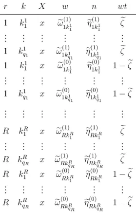
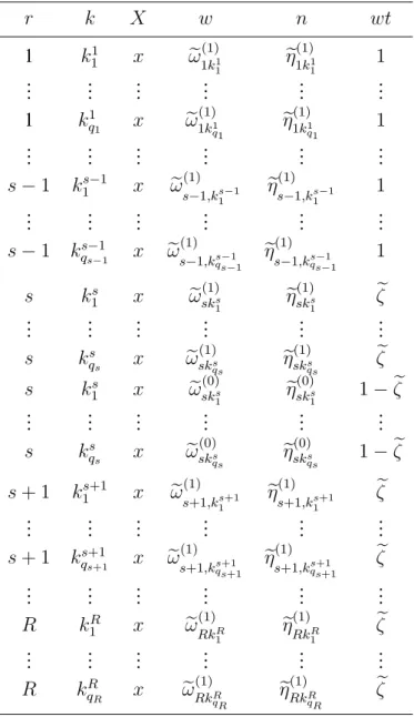
One can construct a pseudo-data frame for each individual as in Table A.1, which can be written more concisely as in Table A.2, with the call

glm(n∼X + factor(k) + offset(log w),weight = wt,family = poisson,link = log)

used to obtain updated estimates ofθ1. In addition, the functionQ2(θ;eθ)is

Q2(θ;θe) = m X i=1 hni_X−1 j=0

logP(Zij = 1|H(t−ini),Z¯i,j−1 = 1j−1, dN(tini) = 1)

+ζe_ilogP(Z_ini = 1|H(t−_ini),Z¯_i,ni−1 = 1_ni−1, dN(t_ini) = 1) + (1−ζe_i) logP(Z_ini = 0|H(t−_ini),Z¯_i,ni−1 = 1_ni−1, dN(t_ini) = 1)

i . Again we construct a pseudo-data frame as in Table A.3 and call the glm function

glm(Z∼j + x,weight = wt,family = quasi−binomial,link = logit)

to obtain updated estimates ofθ2. Variance estimation (Louis, 1982) is described in the Supplementary Material.

Table A.1: Pseudo-data frame for recurrent event process for one subject using the proposed method, whereris the index of the inspection interval,kis the index of the piece of the baseline rate,Xis the covariate,wis the expected time at risk,nis the expected number of events, andwtis the weight

r k X w n wt 1 k1 1 x ωe (1) 1k1 1 e η₁(1)_k1 1 e ζ .. . ... ... ... ... ... 1 k_q11 x ω_e1(1)_k1 q₁ eη (1) 1k1 q₁ ζe 1 k1 1 x ωe (0) 1k1 1 e η₁(0)_k1 1 1−ζe .. . ... ... ... ... ... 1 k1 q1 x ωe (0) 1k1 q₁ eη (0) 1k1 q₁ 1−ζe .. . ... ... ... ... ... R kR 1 x eω (1) RkR 1 e η_Rk(1)R 1 e ζ .. . ... ... ... ... ... R kR qR x ωe (1) RkR qR eη (1) RkR qR e ζ R kR₁ x _eω(0)_RkR 1 e η_Rk(0)R 1 1−ζe .. . ... ... ... ... ... R kR_qR x ω_e(0)_RkR qR eη (0) RkR qR 1−ζe

Table A.2: Pseudo-data frame for recurrent event process for one subject using the proposed method (simplified version), whereris the index of the inspection interval,k is the index of the piece of the baseline rate, X is the covariate,wis the expected time at risk,n is the expected number of events, andwtis the weight

r k X w n wt 1 k₁1 x ω_e1(1)_k1 1 ηe (1) 1k1 1 1 .. . ... ... ... ... ... 1 k1 q1 x eω (1) 1k1 q₁ eη (1) 1k1 q₁ 1 .. . ... ... ... ... ... s−1 k₁s−1 x ω_e(1) s−1,ks₁−1 eη (1) s−1,ks₁−1 1 .. . ... ... ... ... ... s−1 ks−1 qs−1 x ωe (1) s−1,k_qss−₋1₁ ηe (1) s−1,ks_qs−₋1₁ 1 s ks 1 x ωe (1) sks 1 eη (1) sks 1 ζe .. . ... ... ... ... ... s ks qs x ωe (1) sks qs ηe (1) sks qs ζe s ks 1 x ωe (0) sks 1 eη (0) sks 1 1−ζe .. . ... ... ... ... ... s ks qs x ωe (0) sks qs ηe (0) sks qs 1−ζe s+ 1 k₁s+1 x ω_e(1) s+1,k₁s+1 eη (1) s+1,ks+1₁ ζe .. . ... ... ... ... ... s+ 1 ks+1 qs+1 x ωe (1) s+1,k_qs+1s+1 ηe (1) s+1,ks+1_qs+1 ζe .. . ... ... ... ... ... R kR 1 x ωe (1) RkR 1 e η_Rk(1)R 1 e ζ .. . ... ... ... ... ... R kR qR x eω (1) RkR qR ηe (1) RkR qR e ζ

Table A.3: Pseudo-data frame for mover-stayer model for one subject using the proposed method, whereZ is the mover-stayer indicator,j is the number of events,Xis the covariate,wtis the weight

Z j X wt 1 0 x 1 .. . ... ... ... 1 n−1 x 1 1 n x ζe 0 n x 1−ζe

R

Andersen, P., Borgan, O., Gill, R., and Keiding, N. (1993). Statistical Models Based on Counting Processes. Springer-Verlag, New York, NY.

Balakrishnan, N. and Zhao, X. (2009). New multi-sample nonparametric tests for panel count data.

The Annals of Statistics, 37:1112–1149.

Barber, C., Geldenhuys, L., and Hanly, J. (2006). Sustained remission of lupus nephritis. Lupus, 15:94–101.

Byar, D., Kaihara, S., Sylvester, R., Freedman, L., Hannigan, J., Koiso, K., Oohashi, Y., and Tsug-awa, R. (1986). Statistical analysis techniques and sample size determination for clinical trials of treatments for bladder cancer. Progress in Clinical and Biological Research, 221:49–64.

Chen, B., Cook, R., Lawless, J., and Zhan, M. (2005). Statistical methods for multivariate interval-censored recurrent events. Statistics in Medicine, 24:671–691.

Cheng, S. and Wei, L. (2000). Inferences for a semiparametric model with panel data. Biometrika, 87:89–97.

Cole, E., Cattran, D., Farewell, V., Aprile, M., Bear, R., Pei, Y., Fenton, S., Tober, J., and Cardella, C. (1994). A comparison of rabbit antithymocyte serum and OKT3 as prophylaxis against renal allograft rejection. Transplantation, 57:60–67.

Conlon, A., Taylor, J., and Sargent, D. (2014). Multi-state models for colon cancer recurrence and death with a cured fraction. Statistics in Medicine, 33:1750–1766.

Cook, R., Kalbfleisch, J., and Yi, G. (2002). A generalized mover-stayer model for panel data.

Biostatistics, 3:407–420.

Cook, R. and Lawless, J. (2007). The Statistical Analysis of Recurrent Events. Springer, New York, NY.

Cook, R. and Lawless, J. (2014). Statistical issues in modeling chronic disease in cohort studies.

Statistics in Biosciences, 6:127–161.

Dempster, A., Laird, N., and Rubin, D. (1977). Maximum likelihood from incomplete data via the EM algorithm. Journal of the Royal Statistical Society, Series B (Methodological), 39:1–38. Gladman, D., Farewell, V., and Nadeau, C. (1995). Clinical indicators of progression in psoriatic

arthritis: multivariate relative risk model. The Journal of Rheumatology, 22:675–679.

Gladman, D., Hing, E., Schentag, C., and Cook, R. (2001). Remission in psoriatic arthritis. The Journal of Rheumatology, 28:1045–1048.

Grossman, R., Mukherjee, J., Vaughan, D., Cook, R., LaForge, J., Lampron, N., and Eastwood, C. (1998). A 1-year community-based health economic study of ciprofloxacin vs usual antibiotic treat-ment in acute exacerbations of chronic bronchitis: the Canadian Ciprofloxacin Health Economic Study Group. CHEST Journal, 113:131–141.

Healey, L. (1984). Long-term follow-up of polymyalgia rheumatica: evidence for synovitis.Seminars in Arthritis and Rheumatism, 13:322–328.

Hogan, J., Roy, J., and Korkontzelou, C. (2004). Handling drop-out in longitudinal studies. Statistics in Medicine, 23:1455–1497.

Hortobagyi, G., Theriault, R., Porter, L., Blayney, D., Lipton, A., Sinoff, C., Wheeler, H., Simeone, J., Seaman, J., Knight, R., Heffernan, M., Reitsma, D., Kennedy, I., Allan, S., and Mellars, K. (1996). Efficacy of pamidronate in reducing skeletal complications in patients with breast cancer and lytic bone metastases. New England Journal of Medicine, 335:1785–1792.

Huang, C., Wang, M., and Zhang, Y. (2006). Analysing panel count data with informative observation times. Biometrika, 93:763–775.

Kalbfleisch, J. and Lawless, J. (1985). The analysis of panel data under a markov assumption.Journal of the American Statistical Association, 80:863–871.

Kessing, L., Hansen, M., and Andersen, P. (2004). Course of illness in depressive and bipolar disor-ders naturalistic study, 1994-1999. The British Journal of Psychiatry, 185:372–377.

Lawless, J. (1987). Negative binomial and mixed Poisson regression. Canadian Journal of Statistics, 15:209–225.

Lawless, J. (2013). The design and analysis of life history studies. Statistics in Medicine, 32:2155– 2172.

Lawless, J. and Nadeau, C. (1995). Some simple robust methods for the analysis of recurrent events.

Technometrics, 37:158–168.

Lawless, J. and Zhan, M. (1998). Analysis of interval-grouped recurrent-event data using piecewise constant rate functions. Canadian Journal of Statistics, 26:549–565.

Lin, D., Wei, L., Yang, I., and Ying, Z. (2000). Semiparametric regression for the mean and rate functions of recurrent events.Journal of the Royal Statistical Society: Series B (Statistical Method-ology), 62:711–730.

Louis, T. (1982). Finding the observed information matrix when using the EM algorithm. Journal of the Royal Statistical Society, Series B (Methodological), 44:226–233.

Park, D.-H., Sun, J., and Zhao, X. (2007). A class of two-sample nonparametric tests for panel count data. Communications in Statistics - Theory and Methods, 36:1611–1625.

Pascual, J., Falk, R., Piessens, F., Prusinski, A., Docekal, P., Robert, M., Ferrer, P., Luria, X., Segarra, R., and Zayas, J. (2000). Consistent efficacy and tolerability of almotriptan in the acute treatment of multiple migraine attacks: results of a large, randomized, double-blind, placebo-controlled study.

Cephalalgia, 20:588–596.

Peters, R., Mehta, S., Fox, K., Zhao, F., Lewis, B., Kopecky, S., Diaz, R., Commerford, P., Valentin, V., Yusuf, S., and Clopidogrel in Unstable angina to prevent Recurrent Events (CURE) Trial In-vestigators. (2003). Effects of aspirin dose when used alone or in combination with clopidogrel in patients with acute coronary syndromes observations from the clopidogrel in unstable angina to prevent recurrent events (cure) study. Circulation, 108:1682–1687.

Pledger, G., Sackellares, J., Treiman, D., Pellock, J., Wright, F., Mikati, M., Sahlroot, J., Tsay, J., Drake, M., Olson, L., Handforth, C., Garnett, W., Schachter, S., Kupferberg, H., Ashworth, M., McCormick, C., Leiderman, D., Kapetanovic, I., Driscoll, S., O’Hara, K., Torchin, C., Gentile, J., Kay, A., and Cereghino, J. (1994). Flunarizine for treatment of partial seizures results of a concentration-controlled trial. Neurology, 44:1830–1836.

Riggs, B., Wahner, H., Dunn, W., Mazess, R., Offord, K., and Melton, L. (1981). Differential changes in bone mineral density of the appendicular and axial skeleton with aging: relationship to spinal osteoporosis. Journal of Clinical Investigation, 67:328–335.

Salvarani, C., Cantini, F., Boiardi, L., and Hunder, G. (2002). Polymyalgia rheumatica and giant-cell arteritis. New England Journal of Medicine, 347:261–271.

Shen, H. and Cook, R. (2014). A dynamic mover-stayer model for recurrent event process subject to resolution. Lifetime Data Analysis, 20:404–423.

Sun, J. and Fang, H.-B. (2003). A nonparametric test for panel count data. Biometrika, 90:199–208. Sun, J. and Kalbfleisch, J. (1995). Estimation of the mean function of point processes based on panel

count data. Statistica Sinica, 5:279–290.

Sun, J., Tong, X., and He, X. (2007). Regression analysis of panel count data with dependent obser-vation times. Biometrics, 63:1053–1059.

Sun, J. and Wei, L. (2000). Regression analysis of panel count data with covariate-dependent obser-vation and censoring times. Journal of the Royal Statistical Society: Series B (Statistical Method-ology), 62:293–302.

Sun, J. and Zhao, X. (2013). Statistical Analysis of Panel Count Data. Springer, New York, NY. Thall, P. and Lachin, J. (1988). Analysis of recurrent events: Nonparametric methods for

random-interval count data. Journal of the American Statistical Association, 83:339–347.

Wellner, J. and Zhang, Y. (2000). Two estimators of the mean of a counting process with panel count data. Annals of Statistics, 28:779–814.

Wellner, J. and Zhang, Y. (2007). Two likelihood-based semiparametric estimation methods for panel count data with covariates. The Annals of Statistics, 35:2106–2142.

Zhang, Y. (2002). A semiparametric pseudolikelihood estimation method for panel count data.

Biometrika, 89:39–48.

Zhang, Y. (2006). Nonparametric k-sample tests with panel count data. Biometrika, 93:777–790. Zhao, X. and Tong, X. (2011). Semiparametric regression analysis of panel count data with

informa-tive observation times. Computational Statistics & Data Analysis, 55:291–300.

Zochling, J. and Braun, J. (2006). Remission in ankylosing spondylitis. Clinical and Experimental Rheumatology, 24:88–92.