Uncertainty propagation through large nonlinear models.

Uncertainty Propagation Through Large

Nonlinear Models

William Becker

A thesis submitted to the University of Sheffield for

the degree of Doctor of Philosophy in the faculty of

Engineering.

Department of Mechanical Engineering

January

2011

Abstract

Uncertainty analysis in computer models has seen a rise in interest in recent years as a result of the increased complexity of (and dependence on) computer models in the design process. A major problem however, is that the computational cost of propagating uncertainty through large nonlinear models can be prohibitive using conventional methods (such as Monte Carlo methods). A powerful solution to this problem is to use an emulator, which is a mathematical representation of the model built from a small set of model runs at specified points in input space. Such emulators are massively cheaper to run and can be used to mimic the "true" model, with the result that uncertainty analysis and sensitivity analysis can be performed for a greatly reduced computational cost. The work here investigates the use of an emulator known as a Gaussian process (GP), which is an advanced probabilistic form of regression, hitherto relatively unknown in engineering. The GP is used to perform uncertainty and sensitivity analysis on nonlinear finite element models of a human heart valve and a novel airship design. Aside from results specific to these models, it is evident that a limitation of the GP is that non-smooth model responses cannot be accurately represented. Consequently, an extension to the GP is investigated, which uses a classification and regression tree to partition the input space, such that non-smooth responses, including bifurcations, can be modelled at boundaries. This new emulator is applied to a simple nonlinear problem, then a bifurcating finite element model. The method is found to be successful, as well as actually reducing computational cost, although it is noted that bifurcations that are not axis-aligned cannot realistically be dealt with.

Contents

Abstract

Acknowledgements

1 Introduction

1.0.1 A mack Box View

1.1 Uncertainty in Computer Models 1.2 Sources of Uncertainty

1.3 Uncertainty Analysis.

1.3.1 Computational Expense 1.3.2 Solutions

· ...

1.3.3 Sensitivity Analysis 1.4 Objectives of this Thesis . 1.5 Summary of Chapters

..

2 Uncertainty Analysis: An Overview 2.1 Issues in Uncertainty Analysis.

2.1.1 Quantification 2.1.2 Fusion . .

_·

_.

2.1.3 Propagation . 2.1.4 Summary

·

_.

2.2 Sensitivity Analysis: an Extension of Uncertainty Analysis. 2.2.1 1Iotivations . . . .

2.2.2 Levels of Sensitivity Analysis 2.2.3 Summary... 2.3 Propagating Probabilistic Uncertainty

2.3.1 General Approaches . . . . v iii ix 1 2 3 4 5 5 5 6 6 7 11 11 12 21 22 23 24 24 25 30 30 30

CONTENTS vi

2.3.2

The Stochastic Finite Element Method.

33

2.3.3

Random l\fatrices. . .

36

2.3.4

Summary of Propagation Methods

36

2.4

Emulators for Uncertainty Analysis.

37

2.4.1

About Emulators .

37

2.4.2

Types of Emulator

38

2.5

Conclusions . . .

41

3 Gaussian Processes and Bayesian Sensitivity Analysis 43

3.1

Gaussian Processes . . . .

44

3.1.1

Prior Specification

46

3.1.2

Conditioning on the Training Data

48

3.1.3

Marginalising Hyperparameters . .

50

3.1.4

Estimating Roughness Parameters

55

3.2

Inference for Sensitivity Analysis

...

56

3.2.1

Mean, Variance and Main Effects.

56

3.2.2

Sensitivity Indices

· ...

59

3.2.3

Derivation of Integrals for Sensitivity Indices

61

3.3

Conclusions . . . .

· ...

66

4 Modelling the Aortic Valve 69

4.1

The Aortic Valve . . . . .

· ...

70

4.1.1

Valve Failure and Prostheses

70

4.1.2

Material Properties. 72

4.2

Simulating the Aortic Valve 73

4.2.1

Existing Work

73

4.2.2

Uncertainties

74

4.3

The Finite Element Models

75

4.3.1

The Dry Model .

76

4.3.2

The Wet Model .

78

4.4

Conclusions . . .

84

5 Uncertainty Analysis of the Aortic Valve Models 87

5.1

Approach

...

87

CONTENTS

5.1.2 Wet model 5.2 Results...

5.2.1 Model Outputs 5.2.2 Dry Model Results 5.2.3 \Vet l\Iodel Results . 5.3 Discussion.

5.4 Conclusions

6 Modelling an Airship 6.1 Airships and Applications 6.2 The Elettra Twin Flyers

6.2.1 Design. . . . .

6.2.2 l\laterials and Uncertainties 6.3 The Airship Models . . . .

6.3.1 Nonlinear Dry Simulation 6.3.2 Nonlinear Wet Simulation 6.4 Conclusions . . . . vii 89 91 91 92 98 .108 · 110 113 · 113 · 114 · 114 · 116 · 119 · 121 · 123 · 127

7 Uncertainty Analysis of the Airship Model 129

7.1 Dry Model. . . 129

7.1.1 VA Approach. . 129

7.1.2 Results . 131

7.2 Wet Model . 135

7.3 Conclusions . 138

8 Tree-Structured Gaussian Processes for Uncertainty Analysis 141 8.1 Classification and Regression Trees . . . 142

8.1.1 Growing Trees - Greedy Algorithms . 143

8.2 Bayesian CART. . 144

8.2.1 Overview . 144

8.2.2 Prior Specification . 145

8.2.3 Searching the Posterior Distribution . 148

8.2.4 Comments on the Posterior Search . 151

8.2.5 Extension to Tree-Structured GPs · 151

CONTENTS

9

8.2.7 Summary of Tree-Structured CPs 8.3 Example: Duffing Oscillators . .

8.3.1 About Duffing Oscillators 8.3.2 Results ..

8.3.3 Discussion. 8.4 Conclusions....

Emulating a Bifurcating System 9.1 Dry Leaflet Model

9.2 Results . . . 9.2.1 Raw Data. 9.2.2 Fitting Emulators 9.2.3 Reduced Training Data 9.3 Conclusions . . . .

10 Conclusions and Further Work

10.1 Emulator-based Uncertainty Analysis. 10.2 Practical Observations . .

10.3 Heart Valves and Airships 10.4 Further Work

References

A Publications

D Practical Aspects of Bayesian Uncertainty Analysis

C The Aortic Valve Model

viii · 155 · 156 · 156 · 156 · 163 · 164 167 · 167 · 168 · 168 · 170 .175 · 178 179 · 179 · 181 · 182 · 182 184 195 197 205

Acknow ledgements

This thesis is the product of some great ideas from some very clever people, and some hard work on my part, particularly inspired by very tight deadlines towards the end. First of all, I would like to thank Keith Worden, who provided the ideas for the vast majority of the work presented here, took the patience to explain them to me when necessary (quite often, in fact!) and was always kind enough to take me and other students for curries, meals and pub visits in Sheffield and beyond. It truly has been a privilege to work with such a hugely intelligent but extremely friendly and approachable man such as Keith, who will always do his utmost to help out ailing PhD students. I will very much miss working with him when I move away from the group. I also express my thanks to Graeme Manson, who as my other supervisor was always available for help when needed.

On the academic front, thanks must go to Jeremy Oakley, who was one of the main creators of much of the theory in Chapter 3, also for his patience in attempting to explain Bayesian statistics to a newly-graduated student with an A-level statistics education. I also gratefully received much help from James Hensman concerning Gaussian processes, although many times it went over my head! For the latter stages of my PhD I would like to thank the members of "Bayes Club", which also included Rob Barthorpe and Lizzy Cross. These discussions helped me enormously with the latter chapters of this thesis and were also very enjoyable.

For help on the FE side of things, thanks go to Alaster Yoxall for his advice on heart valves and modelling, and Jen Rowson for help with LS-Dyna. I must also thank James Kennedy from KBS2 Inc. for his extremely generous assistance via the LS-Dyna forum on numerous aspects of the use of LS-Dyna, which, incidentally, is woefully under-documented.

A special thanks goes to Jem Rongong, who firstly helped with funding in the latter stages of the PhD, and secondly was very understanding about my time restrictions in the final two months.

Thanks must inevitably go to all my friends in the department who have helped me over the years with endless tips and assistance with various software packages and matters relating to general PhD life. But much more valuably, they have made working in this research group a wonderful experience. I can only hope that my next working environment will be comparable. Specific thanks must go to the members of Lunch Club: the leaders

x Vaggelis (Blue) and Giovanni (Pink) for being my best friends over the past three years, plus the more peripheral members Pete, Rob and Dorit for plenty of good trips to the pub. Lunch Club alumni must also be mentioned - Frank Stolze provided endless help and jokes in the office and is very much missed, as well as gli Italiani. All these people have made working in the DRG a great experience. Thanks to all the people in my office for putting up with my grumpiness in the last months of thesis-writing!

I must also thank the people who I met in Torino. Cecilia Surace and David Storer for their warm welcome and endless help, including several excellent ski outings. All the Italians for inviting me for excellent dinners of vast proportions, particularly Marco Gherlone and Maria De Stefano. I must also thank Melegcim for being such an excellent friend throughout the last few months of the visit and beyond.

Thanks also go to all the people who were not directly involved in the thesis, but have been great friends and family throughout, which inevitably helps. My Mum and Dad have always been there for me and I love them dearly. My brother Alex and Dave (members of Magiklegz) are my oldest and best friends and I can count on them for anything. I should particularly thank Valeria Amenta, who was probably the only thing stopping me going crazy at a few points in the last months. Grazie mille Tortigliona!

I would like to thank Ove Arup for the use of LS-Dyna. The activity presented in Chapters 6 and 7 was part of the project entitled "Innovative Solutions for Control Systems, Electric Plant, Materials and Technologies for a Non-Conventional Remotely-Piloted Aircraft" funded by the Piedmont Region of Italy. A large part of the work here was funded by a Platform Grant for uncertainty management in nonlinear systems. Funding also came from the "Bridging the Gaps" initiative.

-p.s. Although I can't exactly thank my dog for any academic input, I would like to dedicate this thesis to Bess, who is sorely missed.

Acronyms

ALE Arbitrary-Lagrangian-Eulerian

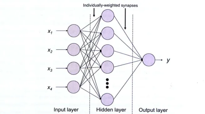
ANN Artificial Neural Network

APDL Ansys Parametric Design Language

BBA Basic Belief Assignment

CART Classification And Regression Tree cdf Cumulative distribution function

COY Coefficient Of Variation

CV Cross-Validation

DOE Design Of Experiments

DST Dempster-Shafer Theory of evidence

EOS Equation Of State

ETF The Elettra Twin Flyers {The airship design from Chapter 3

FE Finite Element

FSI Fluid-Structure Interaction

FRF Frequency Response Function GP Gaussian Process

iid Independent and Identically Distributed KL Karhunen-Loeve (expansion)

LHS Latin Hypercube Sampling

LLM Limiting Linear Model LTA Lighter Than Air

MAP Maximum A Posteriori MCMC Markov Chain :Monte Carlo MEl Main Effect Index

MH Metropolis-Hastings

MLE Maximum Likelihood Estimation OAT One-At-a-Time

PCE Polynomial Chaos Expansion pdf Probability density function

RJ-MCMC Reversible-Jump Markov Chain Monte Carlo RMS Root-Mean-Squared

SA

Sensitivity Analysis

SFEM Stochastic Finite Element Method

SSFEM Spectral Stochastic Finite Element Method ST Soft Tissue (material model)

TSI Total Sensitivity Index U A Uncertainty Analysis

Nomenclature

IL Vector of means of a multivariate probability distribution ¢(x) Vector of basis function(s) of x

¢r An integral occurring in the inference of sensitivity analysis quantities from the GP

e

The vector of the full set of model parameters

X Matrix of inputs of training data

€ True strain

'fJ A leaf of a classification and regression tree &2 Best estimate of (12

A Deviatoric stretch (equal to 1 + € )

A * Stretch at which collagen fibres are fully straightened in ST model

w

Mean of posterior distribution of w

e A constant in the posterior mean function of the GP

F The deformation gradient tensor

t(x) Vector of the covariance of x with all training data

tr An integral occurring in the inference of sensitivity analysis quantities from the GP w Vector of basis function coefficients or weights

y Vector of model output values of training data x Vector input of a model or function

x

An input point in the vicinity of x x* Input of unknown function value y Vector output of a model or function

V Training data

gp

Gaussian process (distribution notation)

xiv

Ig

The inverse-gamma distribution

N

The normal distribution

U The uniform distribution W The Wishart distribution

X The sample space, or support, of a (possibly multi-dimensional) random variable Xr The support of the joint distribution of the variables Xr where r ~ d

/-L Membership function of a fuzzy set or angle of incident gust on the airship model

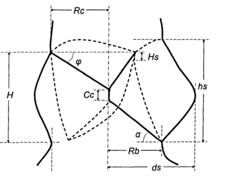
<I> Matrix of basis functions for each sample point <p Angle of leaflet coaptation

p Density

Ew Covariance matrix of posterior distribution of w

E Covariance matrix of a multivariate probability distribution

cr2 _{Scaling factor of the G P covariance function}

e

The universal set, or frame of discernment

It,12 First and second deviatoric invariants of the right Cauchy deformation tensor

A

A fuzzy set

o

The empty set

A An event, or the covariance matrix of a GP

B An event, or the matrix of roughness coefficients in the GP covariance function bi The (i, i) th element of B, corresponding to roughness with respect to the input i c(·, .) Covariance function of a GP

CIS Neo-Hookean coefficient of sinus/aorta material model C5L Post-transition modulus of leaflet material model

c· ( " .) Predictive covariance function of G P (before marginalisation)

c**(·,·) The posterior covariance function of the GP (after hyper parameter marginalisa-tion)

Gl , C2,'" Coefficients of the Mooney-Rivlin material model and ST model d Number of model inputs or function dimensions

E

The expected value

xv

EI Elastic modulus of valve leaflet Es Elastic modulus of sinus/aorta

Fltrad Leaflet separation in relaxed state (ratio)

9 Monotone measure

i An index referring to a particular input variable J Volume ratio (equal to det (F) )

j An index referring to the training data points K Effective bulk modulus

k Number of divisions in a factorial experiment

m*(x) Predictive mean function of GP (before marginalisation)

m**(-) The posterior mean function of the GP (after hyperparameter marginalisation) n Number of training data points

nv Number of training data in the region Tv P(x) Cumulative probability distribution of x

p(x) Probability of x or probability density function of x

P_r An integral occurring in the inference of sensitivity analysis quantities from the GP P D I F Pressure difference scaling factor

q Number of basis functions of x (equal to n + 1 in the examples used)

Qr An integral occurring in the inference of sensitivity analysis quantities from the GP R Number of regions of input space for treed GPs and importance sampling

T A subset of d, i.e. a subset of model inputs or input dimensions r v The v th leaf (terminal node) of a classification and regression tree

Rb Radius of valve base

s Split value at a node in a regression tree

Si Sensitivity index of scaled main effect index of an input Xi

Sr An integral occurring in the inference of sensitivity analysis quantities from the GP STi Scaled total effect index of Xi

T A classification and regression tree Tc Thickness of commissure region Tl Thickness of valve leaflet

xvi Ts Thickness of sinus/aorta

U_r An integral occurring in the inference of sensitivity analysis quantities from the GP v Index of regions in sample space

Vi

Unsealed main effect index of Xi VTi Unsealed total effect index of Xi W Strain energy

X Random variable

X Scalar input of a model or function

xU A column vector comprising of Xr and x~r Y Random variable of (scalar) model output y Scalar output of a model or function

Chapter

1

Introduction

True wisdom consists in knowing that you know nothing. (Bill S. Preston Esq., paraphrasing Socrates - see above)

Perhaps one of the most profound changes to engineering in the 20th century was caused by the advent of computers. Computers have enabled calculations to be performed of a complexity and scale that would have been inconceivable in previous centuries. Fur-thermore, as processing power has increased exponentially, so has the ability to perform increasingly complicated calculations. Finite element (FE) models are a case in point. A very complicated structure may be divided into much smaller and simpler elements, each of which is governed by well-known equations describing displacement and stress as a result of applied forces and boundary conditions. As the availability of computing power has dramatically increased, so the complexity and scale of FE models has followed, to the point where models with millions of elements are no longer seen as exceptional. This trend is reflected in every type of computer model used in engineering today.

Since computer models offer enormous insight into the workings of complicated systems, for a fraction of the cost of prototypes and tests, they are very attractive to engineering

"',,---... "

,

"

X

\

,

\

,

\ L ________________ \ I \ / Material \ / Properties \

:

\ I \

:

\ I \ I I I Model I

!

Dimensions

I

I I I I I I \ I \ I \ I \ Loads / \ I \ I \ I \ I \

,

,

,,'

' ...

_-_

... " Model input variables

(examples) ,.---...

/'

y

"

,

,

,

\

,

\ /---\ / Stresses \ I \ I \ I \ I \

,

\ I I Computer Model

f(x)

I--!-, _Displacements I I I

,

I I I

,

Mathematical equations and assumptions governing model I I I I

,

I I \

,

\ I \ Modes of / \ vibration / \ I \

,

\

,

,

_{, , ,-"} " ----" Model output variables

(examples)

Figure 1.1: A "black box" view of a computer model.

2

industries. Large engineering projects now rely heavily on computer models, which have become an integral part of the design process - examples of such "virtual prototyping" can be found in all major engineering companies.

1.0.1

A Black Box View

All computer mod Is can be considered as systems that take a number of input parameters x

=

{

xd1

=

1

(such as material properties, loads, boundary conditions etc. for an FE

model), and return a number of outputs y (displacements, stresses, velocities etc.), i.e.

y = f(x) (1.1)

Figure 1.1 illustrates this "black box" view. The mapping of the inputs to the outputs

is controlled by a number of mathematical relationships, which can be considered as a

function f(x). There is little doubt that with the increase of processing power it has been possible to greatly increase the sophistication of the equations that dictate the model outputs given some set of inputs - multiphysics simulations can now closely simulate in-teractions between solids and fluids, with magnetic and thermal considerations if required. However, the quality of the model output is also highly dependent on the quality of the

input values themselves, all the more so since more sophisticated models typically require more information to be defined than simpler ones. Consider for example the material definition in an FE model: only a few years ago many materials were approximated as

l.1 Uncertainty in Computer Models

"*1

_E :l ,Q, OJ C 'C Q) Q) C '0, C Q) ,~ I/) C o

~

:0 :l 0. .... Q) .0 E :l Z 1985 1990 1995 Year 2000 2005 3 2010

Figure 1.2: Number of publications per year with "uncertainty" in the title (sourc Scopus [1]) .

being linear due to restrictions in processing power, which requires the definition of only one or two parameters. Modern material models describing hyperelastic and viscoelastic

materials now require a great number of parameters to fully specify the material alone.

1.1

Uncertainty in Computer Models

Given the increased sophistication and reliance on computer models, it is becoming increas

-ingly apparent that uncer'tainties in the model inputs create uncertainty in the outputs and results of the model that cannot be reasonably di counted. This has given rise to the discipline known as Uncertainty Analysis (UA), which has een a considerable surge

of interest in recent years. VA seeks ultimately to quantify the uncertainty in the output

of a model, given the uncertainty in the model inputs, which allows much more informed decisions to be taken based on model re ults. Figure l.2 shows a histogram of publications

with the word "uncertainty" in the title in engineering journals from 1980 to the present day. This illustrates (somewhat crudely, given the concurrent increase in publications in

general) the rise in interest over recent years, reflecting the increasing awareness of the

problem as industry relies more heavily on computer models.

As Bill S. Preston Esq. asserts at the beginning of this chapter, "true wisdom consists in knowing that you know nothing". As engineers, we do not have the luxury of such extreme assertions, but we are responsible for fully accounting for what we do and don't know.

1.2 Sources of Uncertainty 4 This can be a much more difficult task than might first be thought - see Chapter 2. The difficulty of describing "knowns" and "unknowns" was famously described by Donald Rumsfeld:

Reports that say that something hasn't happened are always interesting to me, because as we know, there are known knowns; there are things we know we know. We also know there are known unknowns; that is to say we know there are some things we do not know. But there are also unknown unknowns - the ones we don't know we don't know.

(Donald Rumsfeld, 2003)

Despite earning almost universal ridicule, this statement is actually quite logical and begins to make distinctions between different types of uncertainty. A brief discussion on types of uncertainty follows here, which is continued in Chapter 2.

1.2

Sources of Uncertainty

Uncertainties can occur for a number of reasons. Broadly speaking, they can be di-vided into two categories: epistemic uncertainties, and aleatoric uncertainties. Aleatoric uncertainties are those which arise from natural variability - for example, dimensional uncertainties due to machining tolerances, or inherent geometric variability between simi-lar components. Diomechanical models are an excellent example of aleatoric uncertainty: consider a model of loading on a human bone - the dimensions and material properties vary from person to person, so it is essential to consider this variability if the model is to be generally applicable, rather than applicable to a specific individual.

Epistemic uncertainties, on the other hand, are due to the difference between a model's theoretical approximation and reality; an example of this might be approximating a vis-coelastic material by a simple time-independent model. These can be intentional, to reduce computational expense, or due to lack of knowledge. Some uncertainty can be considered as a mixture from both epistemic and aleatoric sources: it might be known that the ma-terial properties of a component vary from one component to the next (aleatory), but a small sample size may not permit the distribution of this parameter to be known with great accuracy (epistemic uncertainty). Generally aleatoric uncertainties cannot be re-duced, whereas epistemic uncertainties can, by further research to improve the correlation of the simulation to reality.

1.3 Uncertainty Analysis 5

1.3 Uncertainty Analysis

Uncertainty analysis is the discipline of accounting for uncertainty in systems, which often occurs in two steps. First of all, the uncertainty in model inputs must be quantified. Sec-ond, the uncertainty is propagated through the model, resulting in a quantification of out-put uncertainty. Sometimes it is necessary to combine information about uncertainty from different sources and frameworks; this is known as the fusion problem. Regarding quan-tification, the most popular framework is probability theory, since it is well-understood and easily interpreted by anyone with a basic mathematical background. Fusion is also an area of research that is still largely confined to mathematical research groups. As such, the majority of interest from an engineering perspective has been generated by the problem of propagating uncertainty. A much more extensive discussion of these aspects of UA is given in Chapter 2.

1.3.1

Computational

Expense

Perhaps the main sticking-point of uncertainty propagation is however that it can be enor-mously time-consuming from a computational perspective. A large FE simulation may take hours or even days to run for a single set of input parameters. With the consideration of uncertainty, the input x can now be considered as a point in a d-dimensional input hyperspace which is bounded by the upper and lower limits of each uncertain parameter. The propagation of uncertainty involves exploring this input space in order to find how the value of y varies with variations of x. Clearly, the computational cost of doing this rises dramatically with the number of uncertain inputs, to the point where it may be unfeasible without enormous amounts of processing power, or even completely impossible. A good example of this is a fairly recent calculation performed at Los Alamos National Labora-tories to propagate uncertainty through a nonlinear FE model of a weapon component under blast loading. The analysis took over 72 hours on a 3968-processor cluster, using nearly 4000 Abaqus/Explicit licences [2]. Obviously this amount of processing power is not available to many, and even when it is available it may not suffice.

1.3.2 Solutions

In order to alleviate this problem, many approaches to propagating uncertainty for reduced computational cost have been proposed. A large class of these are based on the idea of using a small number of model runs at points in the input space to build an emulator of the model that imitates the function f(x), but at a greatly reduced computational cost. The emulator is then used to explore the input space and propagate uncertainty. This approach has been shown to work well, but is only effective if the emulator accurately

1.4 Objectives of this Thesis 6

reproduces the input/output relationship of the model over the full range of input space. The problem of uncertainty propagation is therefore very closely associated with the dis-ciplines of data modelling and machine learning. In particular, nonlinear models generate response surfaces (the hypersurface of the model output as a result of varying the inputs) that are difficult or impossible to characterise with "conventional" regression models. In the extreme case, the response surface may even bifurcate. There is therefore a necessity to develop ways of performing U A with emulators that can emulate as wide a class of computer models as possible. This is the main motivation of this thesis.

1.3.3 Sensitivity Analysis

A furtherance of VA, known as Sensitivity Analysis (SA), is the concept of finding how sensitive the model output is to each input or set of inputs. SA is very closely tied to VA because it forms part of the prognosis resulting from an VA: often the majority of output uncertainty is caused by only a small set of input parameters, so it is of great interest to focus efforts to reduce input uncertainty on these parameters. SA will therefore feature extensively in the following chapters.

1.4 Objectives of this Thesis

The work in this thesis can be considered from two viewpoints. From the point of view of uncertainty analysis, it aims to outline in detail and investigate the use of new emulator-based approaches that are novel to the field of engineering research. The focus here is on the ability to propagate uncertainty through large nonlinear computer models and perform sensitivity analysis for a reasonable computational cost. The work aims to apply these methods to real FE models in order to test and demonstrate their use on real engineering problems, since these nascent approaches are generally developed in the machine learning and statistics communities, and have been applied very little outside of trivial problems. This first objective may therefore be summarised as,

1. To investigate and apply new techniques for propagating uncertainty through large nonlinear engineering models at a reduced computational expense.

From another point of view, the models developed in the work here are themselves novel, particularly given their consideration of uncertainty. Therefore the application of the emulator techniques is not merely a case study or trivial problem, but offers new insight into the respective problems of each model. This second aim can be stated as,

2. To use the emulator propagation techniques from (1) to offer new insight into the problems of each case study.

1.5 Summary of Chapters 7 FUrthermore, it is intended that by examining and using these techniques in detail, the efficacy of each can be assessed and extensions to the methods suggested where appropri-ate.

1.5

Summary of Chapters

This thesis is structured as follows:

Chapter 2

Uncertainty analysis is explained in depth, with a thorough review of contemporary ap-proaches to the quantification, fusion and propagation of uncertainty. Sem;itivity analysis is then introduced and some common measures of sensitivity discussed. Next, the issue of computational expense is addressed, and some solutions in the engineering literature are outlined. The ideal qualities of an emulator are presented, and the Gaussian process (GP) is introduced as an emulator that fulfils many of these criteria.

Chapter 3

Gaussian processes are introduced in depth, with a step-by-step walkthrough of the Bayesian process of conditioning the prior distribution on training data to produce a posterior distribution-over-functions (Le. training the GP). Next, the marginalisation and estimation of hyperparameters is presented in detail. Finally, the process of obtaining analytical sensitivity and uncertainty mea"lures is given. Overall, this chapter aims to present one of the most complete descriptions of GP-based UA and SA available.

Chapter 4

The first case study for Bayesian UA/SA is presented here, which is the modelling of the aortic valve in the human heart. Two FE models are presented that are both novel in different ways. The first model is a "dry" pressure-loaded model that is specified almost entirely by geometric parameters. A second, "wet" model is a sophisticated fluid-structure interaction model that is at least comparable to contemporary models in the biomechanics literature, using anisotropic hyperelastic material models and considering geometric nonlinearities.

1.5 Summary of Chapters 8

Chapter 5

Uncertainty and sensitivity analyses are performed on both aortic valve models using the GP emulator approach. Geometric, material and loading parameters are investigated and conclusions are drawn from a biomechanical perspective, given that the work here repre-sents the only consideration of uncertainty in heart valve models to date. Observations are also made on the success of the GP emulator: while in general it performs extremely well, the possibility of model bifurcations motivates further work in Chapters 8 and 9.

Chapter 6

A second case study is outlined here, which is a model of an new airship design in produc-tion in Italy. The concept of the design and its applicaproduc-tions are explained. A series of FE models of the airship are presented, which are to be used to assess stress and displacement in the design under normal loading from propellers and buoyancy, with the final model ultimately including fluid loading from a gust impact.

Chapter 7

The airship models from Chapter 6 are subjected to uncertainty analyses, again using the Bayesian approach from Chapter 3. The work here is used to assess the effect of uncertainties in the models in order to make better decisions regarding the design of the ship. Further conclusions are also drawn regarding the use of the GP emulator.

Chapter 8

Given the issue of possible model bifurcations raised in Chapter 5, this chapter introduces an extension to the GP emulator which uses classification and regression trees (CARTs) to divide the input space into more homogeneous regions. The Bayesian approach to CART is demonstrated on a simpler regression tree, then the method is shown to be extendable to the "tree-structured GP" with several alterations. Finally it is demonstrated on a simple case study of a Duffing oscillator that the this new emulator is capable of modelling bifurcating data by creating divisions of input space over bifurcations, whereas a single GP introduces unwanted fluctuations in the posterior mean.

Chapter 9

A case study of a bifurcating FE model is presented to investigate the ability of the tree-structured GP to model data from a real bifurcating engineering model. The model investigates the movement and stress in a rigid-stent prosthetic heart valve, which is known

1.5 Summary of Chapters 9

to bifurcate. The data is used to construct both tree-structured and "standard" GP em-ulators, and the results compared. Finally, a brief study is performed on the effect of reducing training data for the tree-structured emulator. Conclusions about the compara-tive abilities of both emulators are drawn, where it is noted that the tree-structured GP has additional advantages as well as its ability to model bifurcations.

Chapter 10

Conclusions from all chapters are summarised and further work is suggf'sted. The bibli-ography and appendices follow.

Chapter

2

Uncertainty Analysis: An

Overview

This chapter aims to outline in more detail the steps and difficulties involved in VA, and presents an overview of the various approaches that have been developed, with a view to putting the work in the rest of this thesis into context. The main aspects and issues of VA are outlined in Section 2.1, including a review of many of the various frameworks that exist for quantifying uncertainty, the relations between them and the practical details surrounding their implementation. In Section 2.3 the specific problem of propagating probabilistic uncertainty is examined, with recent developments described. The concept of sensitivity analysis is then introduced in Section 2.2 as a natural extension of VA, being a tool to explore in more depth the effects of uncertainties. It will be seen that one of the main stumbling blocks of uncertainty and sensitivity analysis is the problem of computational expense, therefore a class of methods known as "emulator-ba.,.,ed" methods is introduced in Section 2.4. This provides the motivation for the work in Chapters 3 and 8.

2.1

Issues in Uncertainty Analysis

It usually agreed that the process of uncertainty analysis raises three key issues. At the most fundamental level, the magnitude and nature of the uncertainty about a given quantity must be expressed in some mathematical way. This is known as the problem of quantification. Probability theory is undoubtedly the most well-known framework, but there are in fact many alternatives, each with its own advantages and disadvantages. In-deed, some offer considerably more general and flexible methods of expressing uncertainty, in particular the ability to express subtle shades of partial ignorance. However many of these frameworks are relatively recent and some have made only a limited impact outside of largely theoretical examples. An intrinsic problem is that uncertainty should ideally be

2.1 Issues in Uncertainty Analysis 12

prC'cis<'iy expressed, which means that a framework should be able to express the vagueness that exists about a quantity, without adding any unnecessary assumptions, and equally, without bdng over-conservative. A discussion of the main methods of quantification is provided in Section 2.1.1.

Given that for a particular problem a number of different types of uncertainty may be present, each could conceivably be expressed in the uncertainty framework that is the most suitable for that particular quantity. Alternatively, for a single quantity, two measures of uncertainty may exist from different frameworks. This then creates the second problem surrounding UA: that of fusion. This is the problem of translating from uncertainty expressed in one framework to another in order to fuse the data from the two frameworks into a single, more informative expression about uncertainty in that variable. It is evident that the various frameworks discussed here are related to each other in many ways; in fact, s01l1e may be seen as special ca"les of other more general theories. Although the fusion problem is almost certainly the least-investigated problem of the three mentioned here, a short overview of recent developments is given in Section 2.1.2.

Finally, the problC'm known as propagation is usually the subject of the most interest in the field of engineering. In short, if the uncertainty in some model inputs has been quantified in some way, what will be the uncertainty in the outputs and results of the model? This problC'm is undoubtedly the most studied because it gives the end product of uncertainty analysis: the output uncertainty. For a system that can be expressed in terms of a set of tractable equations, uncertainty can be propagated analytically. In most cases however, models are not analytically tractable and can be viewed even as unknown functions of their inputs - unknown in the sense that for a particular set of input values the output is not known until the model has been run. The problem is further compounded by nonlinearities in the model response: small variations in inputs can cause disproportionately large variations in any of the model outputs and even bifurcations. This leads to the general class of propagation techniques known as sampling-based approaches. As will be seen, the main hurdle to be overcome is that the accuracy of propagation is strongly related to computational expense, so much so that standard methods can quickly become unviable for large problems. This is discussed at length in Section 2.4. A discussion of methods of propagation is given in Section 2.1.3.

2.1.1

Quantification

A brief outline is given here of some of the main frameworks for dealing with uncertainty. Although probability theory will be used throughout this thesis for reasons stated later, to put this work in context in the wider field of uncertainty analysis it is useful to briefly examine the alternative theories that are available for dealing with quantification of uncer-tainty. Klir and Smith compare various theories and categorise them in two "dimensions"

2.1 Issues in Uncertainty Analysis 13

FORMAUSEDLANGUAGES

UNCERTAINTY THEORIES _{Classical Rough Fuzzy rough Rough fuzzy}

sets Fuzzy sets sets sets sets

»

_Probability C _Classical C Classical numerical probability theory based :::j _{probability on fuzzy} <: theory m events

Classical Fuzzy-set

Possibility/necessity possibility interpretation

of possibility

~ theory theory

0

Z Dempster- Fuzzified

0 _{Belief/plausibility} Shafer theory of Dempster --I

0 evidence Shafer theory

Z

m Z Formalisation of

~ 0 Capacities of various _imprecise

m z orders

» :>

probabilities

en C 0

~ c _{Coherent upper and} Formalisation of

m :::j _imprecise

en _<: lower probabilities _{probabilities}

m

Closed convex sets of Formalisation of

probability imprecise

distributions probabilities

etc ..

Figure 2.1: Classification of uncertainty th ories a cording to Klir an I Smith [3] [3] as shown in Figure 2.1. The fir t dim nsion deal with the lassifi ation of set . In cl

as-sical crisp probability th ory, for xample, a probability i' as 'ign d to a 'ubs t of vents

in some universal et. This concept can b ext nd d to as ign probabilitie to fuzzy s l ,

known as probability theory based on fuzzy v nt [4]. Aside from fuzzy . ts, 7'ough s ts (sets where the upp r and lower bounds are themselve d fin d by sets) [5] and fu 'ions

of the two approach s (rough fuzzy sets andfuzzy TOugh sets [6]) ar alternativ ways of

defining uncertainty on a et. Fuzzy et are di u d later in this tion, but rough ets will not b further discussed, sin e th y ar a r latively recent d v lopm nt. Th

interested reader can however refer to [7].

The other dimension deal with the me ur m nt of uncertainty as 'igned to a given t of

ev nts (be ita cri p, fuzzy or rough et etc.). Thes are defin d as rnonoton rneaSUT' , because they satisfy the condition of monotonicity with r p ct to ub thood ord ring, i.e. for all subsets A and B in some universal et

e

,

if A ~ B, th n a monotone measure

9 is such that g(A) ~ g(B).

Monotone measures may be divided into additive and non-additive m asure . For example,

classical probability theory uses an additive measur , i.e. for two vent A and B,

2.1 Issues in Uncertainty Analysis 14

whereas the more general non-additive branch of monotone measure theory allows for cases where g(A U B) =1= g(A) + g(B), therefore capturing types of uncertainty that cannot be dealt with by probability theory alone. Not all of the theories in Figure 2.1 will be discussed here, since a number of them have made little progress beyond the mathematics literature. Instead, only a selection of the main frameworks that have been applied to engineering will be discussed. The subject of quantification is however discussed in much more detail in a recent book by Klir [8].

Interval Theory

One of the most basic expressions that can be made about uncertainty in a variable is that it is within an certain interval. For example, given an uncertain quantity x, it might be known that it lies between an upper bound

x

and a lower bound ~, but no other information is available. Such expression of uncertainty underlies the concept of interval analysis, which was outlined to a large extent by Moore [9] in 1966. More formally, an interval xl is expressed as,

(2.2)

The concept of intervals on scalar quantities can be extended to interval vectors and interval matrices, for example the d-dimensional interval vector

xl

is expressed as,

31=

(2.3)

Thus, whereas a crisp (deterministic) vector will describe a point in d-dimensional space, an interval vector describes a d-dimensional hypercube which is bounded by the upper and lower limits of each component of the vector. Perhaps the most significant limitation of interval analysis is that it is an extremely crude method of specifying uncertainty, merely between one value and another. However, this could also be viewed as an advantage in the case where upper and lower limits are the only information available (which is not an uncommon situation). Interval theory will be seen to be closely related to fuzzy set theory - in fact, perhaps the main application of interval analysis in recent literature is as a basis for implementing fuzzy set theory (see later).

Probability Theory

Probability theory is certainly the most widely-used and well understood method of quan-tifying uncertainty. An uncertain random variable X in some sample space X (the set of all possible outcomes of X) is assigned probabilities p(X) for each value of X EX, such

2.1 Issues in Uncertainty Analysis that, p(x) -+

[0,1] V

x E X LP(x) = 1 xEX 15 (2.4)

In the case when X is continuous, probabilities cannot be assigned to point values of x. Therefore it is convenient to define the probability distribution of x in a number of ways, for example, the cumulative distribution Junction (cdf) P(x) describes the probability of X being equal to or below x. More commonly however, a probability density Junction (pdf) p( x) is used. It is a function that defines the probability of X falling inside a given interval [x, x + <5x], such that,

l

x

+.s

x

p{X E [x, x + &x]} = x p(x)dx (2.5) The univariate case can be generalised to a multivariate pdf for a d-dimensional random variable (hereafter pdf will refer also to the multivariate pdf) denoted p(x), which gives the individual pdfs of each variable Xi and the dependencies between them. An example of this is the multivariate Gaussian distribution, which is given here (since it will feature significantly in this thesis),

(2.6) where J-L is a d-dimensional vector of means and ~ is a dxd covariance matrix that gives the covariance between inputs. An important aspect of multivariate pdfs that will be stated here is the idea of marginalisation, which is stated as,

p( x,.)

=

1

p( x)dx_r X-r

(2.7) which states that the distribution of x,.

c

x can be obtained by integrating with respect to the variables in the complementary set X-r over their sample space

x-

_{r •}

An important distinction in probability theory that should be mentioned here (and the source of ongoing dispute) is the difference between the Jrequentist and Bayesian inter-pretations of probability. From the frequentist perspective, probability is defined as the limit of frequency of occurrence of an event over a large number of trials. This of course introduces the limitation that probabilities of events that have not been witnessed yet cannot be formally specified. In the alternative Bayesian viewpoint, probability is consid-ered to be a degree of belief. Probabilities and distributions can therefore be assigned to events about which there is some subjective opinion or prior knowledge. Bayesian infer-ence, which is the process of inferring unknown quantities through prior assumptions and further evidence, is used extensively in this thesis. Briefly, inference is performed using

2.1 Issues in Uncertainty Analysis 16

an updating procedure known as Bayes' Theorem, such that the probability of an event

B

given some evidence

A

is given as,

(BIA) = p(AIB)p(B)

p p(A) (2.8)

where p(BIA) is called the posterior probability (of B), p(AIB) the likelihood, p(B) the prior probability and p(A) is a normalising factor. Bayes' theorem is often used to estimate model parameters

e

through Bayesian inference, sometimes by finding the posterior mode of

E>,

a process known as maximum a-posteriori (MAP) estimation (see [10]).

A probability distribution is considerably more informative than the intervals described previously. The pdf p(x) can take any number of forms so long as the pdf integrates to lover

X.

This means that potentially any distribution of probability can be expressed, as long as a suitable pdf can be defined. Much like interval analysis, the main strength of probability theory is also its weakness, although in this case the issue is that uncertainty must be expressed in some detail. Even the simplest pdf, the uniform distribution, implies that probability is uniformly distributed within a given range. Interval theory, in contrast, makes no assumption whatsoever about the distribution of uncertainty inside the interval. In the case where detailed information is available about the uncertainty of a parameter, probability theory is an excellent choice. However, quite often the distribution of a variable is unknown and must be elicited. This is itself an active field of research - a full treatment is given in [11]. Even then, a lack of information can force assumptions to be made about the nature of uncertainty in a variable that cannot be justified by the available data.

Possibility Theory

First outlined in detail by Lotfi Zadeh [12], possibility theory is viewed as an alternative to probability theory that allows for more subtle expressions of uncertainty and partial ignorance. Whereas probability theory allows only a single measure of uncertainty (the probability of an event), possibility theory uses two measures, known as the possibility and the necessity. The possibility measure of an event A from the universal set

e

is defined such that pos(A) -+ [0,1], in much the same way as probability. However, a probability measure of 1 suggests that an event is certain to happen, whereas a possibility measure of 1 only suggests that it is completely possible that this event occurs, or in other words, one would not be at all surprised if the event occurs. This can be stated as:

• pos(A)

= 0 implies that

A

is completely impossible

• pos(A) = 1 implies that A is completely possible, plausible or unsurprising

Possibility can of course take any measure in the interval [0, 1], expressing varying degrees of belief about the possibility of A occurring. To complement the possibility, the necessity

2.1 Issues in Uncertainty Analysis

z-'e;; en Q) u Q) Z If possible, is likely to occur

Values on these axes are not allowed

I

Implausible

.

/.

Certain to occur Impossible

I

Ignorance

I

./

o

_o

---~----~---~----~---~----~---~--. 1 Possibility

Figure 2.2: Interpretation of variou regions in po sibility/necessity.

must also be expressed. This is defined as,

nec(A)

= 1

- po (A)

17

(2.9)

where

A

here denotes the complement of A in the universal set. Between the two measure ,

it is possible to express more subtle levels of unc rtainty than with probability theory.

Consider three situations:

• pos(A)

=

0 implies that A is impossible. nee (A) must also be zero.

• pos(A)

=

1 implies that A is completely possible. nec(A) can take any value. If

nec(A)

= 0

, this implies complete ignorance about A, i.e. A is definitely possible,

but it would be completely unsurprising if it did not occur.

• nee (A) = 1 implies that A is completely n cessary and therefore will definitely

occur. This requires that pos(A) = 1.

An illustration of this is given in Figure 2.2. Possibility mea ures follow a serie . of rules,

much like in the probabili tic framework, that allow unions of possibilities, intersections and conditional pos ibilities. For further information, see

[13].

Fuzzy Sets

Fuzzy set theory was first introduced by Lotfi Zadeh [14] (also one of the principle de

2.1 Issue's in Uncertainty Analysis 18 o~

__

~

________________________

~

____ -.

x o~

__

~~

__________________

~

______

+

x

o~

____

~

__________________

~

______

~

x

Figure 2.3: Illustration of nlf'mbership functions of fuzzy quantities: general fuzzy quantity (top); fuzzy number (middle); fuzzy interval (bottom).

cith('r d('finitely belongs or definitely does not belong to a given set, a fuzzy set has an associated membership function that states the degree of membership or belonging to the set IlS a vallie in the interval [0, 1

J.

Thus a "crisp" (conventional) set can be seen as a sIwcial (~ase of a fuzzy set, wh('re an element's membership is only allowed to take a value of eitiH'r 0 (it is not in the s('t) or 1 (it is in the set). A fuzzy set

A

is written as,

(2.10)

where II A is the membership function that a"lsigns a membership value to any x. As with other frameworks for uncertainty, fuzzy sets have a system of rules governing operations such as unions and intersections of sets. The reader is referred to Klir's book [15] for furth('r information. It is important to point out here that the membership function of a fuzzy set is not equivalent to the probability distribution of a random variable (which is a common misunderstanding). The difference is subtle but important: whereas a fuzzy set assigns levels of membership to known and fixed elements of the universal set

e,

probability theory a"lsumes a crisp set, but it is the values of the elements of e that are uncertain. Therefore, fuzzy sets should not be viewed as an alternative to probability theory; rather, the two can complement each other to a large extent. This is discussed in d('tail in [16].

2.1 Issues in Uncertainty Analysis 19 of fuzzy quantities. Fuzzy quantities are a special case of fuzzy sets, since a fuzzy quantity can be thought of as a fuzzy subset of lR. A membership function can be defined ov('r sOllie range of values to express the uncertainty surrounding some particular input paranH'ter (see Figure 2.3). In particular, if the membership function is triangular, it is terIlH'd a Juzzy number, whereas if it is trapezoidal it is referred to as a fuzzy interval (although fuzzy intervals are also sometimes referred to as fuzzy numbers). Fuzzy quantities have been used extensively in UA in engineering - some instances include fuzzy finite d(,llH'nt analysis applied to vibration analysis [17] and fault diagnosis using fuzzy logic [18J. Fuzzy quantities do have the disadvantage however that they force quite strong assumptions about the nature of the membership function and therefore ideally require cousiderable knowledge of the distribution of the quantity of iuterest.

Non-Standard Fuzzy Sets

It is worth briefly mentioning some of the extensions of fuzzy S(·ts that have b('(,11 pro-posed. In the first instance, interval-valued fuzzy sets are fuzzy sets wh('re the llIC'miwrship function is itself uncertain, and assigns an inter-val of meml)('rship rathC'r than a crisp llIem-bership value. Another way of looking at this is to (!<·fine the lI}(,lIllwrship fUllction as an interval,

(2.11)

If this is not uncertain enough, there exist type-2 Juzzy sets, in which the llI(,llll)(,fship function is itself defined on fuzzy intervals. Then·fore, for a giv('n x, the llwnil)('rship function will return a fuzzy quantity dC'scribing the ll1ell1b('rship lew'l of x. In fact, this concept can be extended to further nested levels of membership fUIIctions, although the practical value of this is questionable.

Another extension, known as a level-2 fuzzy set, is to define a numl)('r of diff('rent levd-1 (standard) fuzzy sets, which are themsC'lves groupC'd together into a fuzzy s('t. This nesting of fuzzy sets allows higher-order concepts to be r<'presented by lower-lev£'! OI1('S. As with type-2 fuzzy sets, level-2 fuzzy sets can naturally be extend('d to further levels as required, but again these higher orders have seCl1 little investigation a.'i yet. Some further manifestations of fuzzy sets are discussed in [8].

Dempster-Shafer Theory of Evidence

Dempster-Shafer Theory (DST) is a theory of evidence based on work by Dempster [19] and Shafer [20] in the 19GOs and 1970s. Like possibility throry, DST allows a slightly more general framework than probability theory since it is non-additive and then·fore allows more subtle expressions of partial ignorance. A particular distinction is that instead of only assigning probability mass to single elements, probability mass can be assigned to

2.1 Issu('s in UucC'rtainty Analysis 20

sub.'lds of elcllwnts.

L(,t t he frame of discernment H (othC'rwise known as the universal set in other frame-works) be dditwd as the ('xhaustive s('t of pm;sible events. The elements of {28}, which

arc all the possible subsets A of H, are given a probability mass m known as the basic bdifJ assignment (I3I3A), such that

m(A) ~ [0,1] 'V A ~ 8 m(0) = 0

Lm(A) = 1 A~B

(2.12)

wlH're 0 i:; the empty set. Any subset A of 8 where m(A)

>

0 is called a focal element. If all focal E'il'llwnts arc singletons (Le. contain only one element), this is the special case of I3ay<'sian probability theory - i.e. fl.'!signing belief to single events or non-overlapping suhs(,ts of ('wnts. DST th('refore extends probability theory by allowing a degree of un-c('rtainty or ignorance, because helief in events can "overlap" between different subsets. Partial ignorance is often r<'presmtcd by assigning a proportion of the unit belief mass to the ('utire fmme f), since this implies no special knowledge about any subset of 8. Tlw bdifJ of an eV('Jlt D is related to the DI3A of subsets of A by,

Dd(D) =

L

m(A) (2.13)

A<;H

which SUIll:; all the probability mfl.'!s that is in support of n occurring. A further measure, kuown fl.'! the plausibility, is defined as,

PI(D) =

L

m(A) (2.14)

AnHI0

whi('h expr('ss<'s the total belief mass that could be assigned to

n

if all unknown facts we're found to support D. Finally, a third measure is sometimes used, known as the doubt, whieh is related to the belicf such that,

Dou(D) = Bcl(D) (2.15)

i.e. the total probability mass in support of D not occurring. It should be emphasised that since belief and doubt do not necessarily sum to unity, DST can represent an interval of uncertainty that is beyond the scope of probability theory (see Figure 2.4). In fact, belief and plausibility actually r<'present the upper and lower bounds of the "true" belief in an event. The probability mass assigned to the belief and doubt is fixed, but if the ignorance wcre somdlOw removed (by gaining further information) the remaining mass

2.1 Issues in Uncertainty Analysis 21

o

1

I

Belief Ignorance/uncertainty

I

Doubt

'---

-.."..---~

Plausibility (potential belief)

Figure 2.4: Dempster-Shafer a signment of belief and un rtainty across th unit interval

(adapted from [21]).

could be assigned to either further doubt in an event, or furth r support, so that the trn belief of B can be anywhere in the int rval

[B

I(B), PI(B)J.

DST has been successfully applied in th cont xt of damag 10 atiol in air raft [21], fault

diagnosis in engines [22J and fault diagnosi in induction motor' [23J. H w v r it still

remains largely within the confines of simple th or tical appJi ati n .

2.1.2 Fusion

As stated previously, fusion between th variou th ori fun rtainty is h I a·t illV

/;-tigated of the three problems of UA. The Klir diagram in Figur- 2.1 do ' how vcr 8h w that, in particular, there has been some work done to apply th th ory f fuzzy . ts to

non-additive measures of uncertainty. For xample, Zad h g n rali d prob bility tll-ory

in 1968 to apply to event bounded by fuzzy s ts [4J. Th r lati n and mi und rstand

-ings between fuzzy ts and probability theory ar di ' U" d in som d tail by uboi

[16J. Zadeh similarly interpreted classical possibility th ory in a fuzzy nt xt [12J a !ittl later, and more recently has suggested a Gen mlised th ory of unc rtainty [24J. D T has

also recently been generali ed to d al with fuzzy ts, pr rving th con pt of upp rand

lower probabilities (which had previou Iy not b n a h iv d). Mol' on thi an b found

in [25J.

There are also some cross-over between various th orie of monoton measur s. Ro .' has

done work to create a bridge between probability and po ibility th ory in th ont xt of

"Total Uncertainty" [26], which allows an expr s ion of both epi temi un rtainty and aleatory. Dubois also discusse at length the variou way in whi h po ibili ti mea ur can be interpreted in a probabilistic sen e [27]. In fact, possibility theory ha be n propos d as a kind of bridge between probability theory and fuzzy set theory by Dubois and Prade [16J. Finally, it has already been stated that DST i' a generali ation of pI' bability th ory to allow non-additive measures of uncertainty. A much full r discus ion of un rtainty

2.1 Issues in Uncertainty Analysis 22

measures and the various associations between them is given in [8J.

2.1.3 Propagation

Intervals

The method of propagation is strongly dependent on the framework of quantification of uncertainty. In the case of interval analysis a system of interval arithmetic parallels many of the arithmetic operations available to crisp numbers. For example, the addition of two intervals is achieved by,

[a, bJ

+

[c, dJ = [(a + c), (b + d)J (2.16) and multiplication is defined by,

[a, bJ

*

[c, dJ = [min(ac, ad, bc, bd), max(ac, ad, bc, bd)J (2.17) Intervals can therefore replace crisp numbers in the specification of model inputs, and theoretically all the calculations that are involved in the solution of the model with the crisp input could be replaced by interval calculations, thus yielding an interval vector that specifics all the outputs of a given model in terms of intervals.

One problem with propagating intervals through a model is that in order to precisely propagate them it is required that the equations governing the model can be expressed in a closed form, but in practise this is rarely possible. Instead, research focuses on approxi-mations of the exact solution set. Additionally, interval analysis introduces conservatism, which means that it tends to over-estimate the uncertainty in the model output as a result of neglecting dependencies between the inputs. Some work has been done to address this last issue by Manson in the context of affine arithmetic [28J. An extensive discussion of the m;e and application of interval analysis is found in [29J.

Fuzzy Quantities

Fuzzy quantities that are assigned to uncertain model parameters can be propagated through a standard FE model by dividing the membership functions into a series of "a-cuts", such that the membership function for each fuzzy input {Xl, X2, ... , xn} is intersected at a level !1Xj = a (see Figure 2.5). This results in number of nested crisp sets at each a-cut that are typically propagated through the model by an interval analysis, producing a realisation of the fuzzy quantities that describe the model outputs. The problem with this is that since it involves interval analysis, it introduces conservatism into the estimates of the output uncertainties (as discussed earlier). A way round this is to use global optimisation to search for the global maximum and minimum of the output at a given a-cut, which means that the practice of propagating fuzzy numbers is closely tied to the discipline