NBER WORKING PAPER SERIES
MIGRATION AND TRADE IN A WORLD OF TECHNOLOGICAL DIFFERENCES:
THEORY WITH AN APPLICATION TO EASTERN-WESTERN EUROPEAN INTEGRATION
Susana Iranzo
Giovanni Peri
Working Paper 13631
http://www.nber.org/papers/w13631
NATIONAL BUREAU OF ECONOMIC RESEARCH
1050 Massachusetts Avenue
Cambridge, MA 02138
November 2007
We thank Gustavo Ventura for sharing with us some unpublished results from his work and Gregory
Wright for his suggestions. Peri acknowledges the John D. and Catherine T. MacArthur Foundation
for financial support. The views expressed herein are those of the author(s) and do not necessarily
reflect the views of the National Bureau of Economic Research.
© 2007 by Susana Iranzo and Giovanni Peri. All rights reserved. Short sections of text, not to exceed
two paragraphs, may be quoted without explicit permission provided that full credit, including © notice,
is given to the source.
Migration and Trade in a World of Technological Differences: Theory with an Application
to Eastern-Western European Integration
Susana Iranzo and Giovanni Peri
NBER Working Paper No. 13631
November 2007
JEL No. F16,F22,J31,J61,O52
ABSTRACT
Two prominent features of globalization in recent decades are the remarkable increase in trade and
in migratory flows between industrializing and industrialized countries. Due to restrictive laws in the
receiving countries and high migration costs, the increase in international migration has involved mainly
highly educated workers. During the same period, technology in developed countries has become progressively
more skill-biased, increasing the productivity of highly educated workers more than less educated
workers. This paper extends a model of trade in differentiated goods to analyse the joint phenomena
of migration and trade in a world where countries use different skill-specific technologies and workers
have different skill levels (education). We calibrate the model to match the features of the Western
European countries (EU-15) and the new Eastern European members of the EU. We then simulate
the effects of freer trade and higher labor mobility between the two regions. Even in a free trade regime
the removal of the restrictions on labor movements would benefit Europe as a whole by increasing
the GNP of Eastern and Western Europe. Interestingly, we also find that the resulting skilled migration
(the so-called "brain drain") from Eastern European countries would not only benefit the migrants
but, through trade, could benefit the workers remaining in Eastern Europe as well.
Susana Iranzo
Universitat Rovira Virgili,
Avda. Universitat 1,
Reus 43204, Spain
[email protected]
Giovanni Peri
Department of Economics
University of California, Davis
One Shields Avenue
Davis, CA 95616
and NBER
1
Introduction
International migrations between less developed and industrialized countries have increased substantially in the last decades. As of 2005, 190 million people lived outside their country of origin, whereas in 1970 this number was only 82 million.1 However, migratory flows increased very little when compared to trade, foreign direct
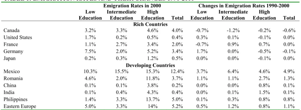
investment and financial capital flows, which represent the other major aspects of globalization. As of 2000, countries overall were selling and buying abroad a value equal to 27% of their gross domestic product and were investing about 20% of their total savings abroad. Yet, as measured by Docquier and Marfouk (2005), in 2000 only 1.8% of the world population was living in an OECD country that was not their country of birth. These differences are to a large extent the result of migratory policies. While developed and, increasingly, developing nations have moved towards greater freedom of trade and capital movements, countries still consider it part of the normal exercise of their sovereignty to restrict drastically the access of immigrants to the domestic labor market. In general, the few successful attempts to relax immigration restrictions have been in the direction of allowing entry to a larger number of highly educated immigrants (e.g., H1B visas in the U.S., the point system in Canada and Australia, and the ”Highly Skilled Workers Program” in the UK). Highly educated migrants are also the fraction of the labor force with the highest degree of international mobility and, we argue in this study, are the most poised to gain from migration. Some representative statistics in Table 1 show that the segment of highly educated individuals coming from less developed countries have been more internationally mobile, and increasingly so in recent decades. The table reports the emigration rates by educational group for several countries2. Emigration rates are calculated as the stock of people residing abroad divided by the working-age
population of the country of origin. The table distinguishes between less educated (0 to 8 years of schooling), those with intermediate education (9 to 12 years of schooling) and the highly educated (13 years of schooling or more). The upper part of Table 1 reports emigration rates and their changes for five representative rich countries. The rates are mostly small and exhibit small changes during the last decade with no clear pattern across educational groups. Overall, advanced countries do not have much emigration in any educational group, and that did not change much during the 1990s. By contrast, the set of less developed countries shows larger emigration rates, especially for the highly educated, and faster growth of those rates during the 1990s. This tendency is particularly strong for China and India where the emigration rate among the highly educated is ten times larger than among the other groups. For Romania, a typical Eastern European economy, and for Eastern Europe as a whole, the emigration rates of the highly educated are two to three times the emigration rates of the less educated. Most of the highly educated Eastern European migrants are now in Western Europe and, as barriers to labor mobility are dismantled as the transitional arrangements of the accession treaty come to an
1The numbers relative to overall world migration reported in this section are from Freeman (2006).
2The data are from Docquier and Marfouk (2005) who collected information from censuses of resident populations in OECD
end,3theflow of highly educated workers to the West is expected to increase.
The migration of highly skilled workers, often called ”brain drain”, has attracted the attention of policy-makers and economists (see Beine et al., 2001). The cost of losing the best educated workers is considered to be high for the sending countries. At the same time, though, several economists recognize that from a world perspective international restrictions on labor mobility are one of the most costly economic distortions (e.g., Klein and Ventura 2007, Kremer and Watts 2006, Benhabib and Jovanovic 2007). Yet, we still lack a clear economic theory that explains migration incentives for the highly educated and their effect in a world with trade and technological differences across countries. This paper develops such a model, calibrates it to match existing economies, and simulates it to obtain some comparative statics results that illustrate the effects of removing barriers to labor mobility.
We propose a two-country (”Rich” and ”Poor”), two-sector (”Traditional” and ”High-tech”) model with heterogeneous workers and skill-specific technological differences across countries. In particular, the Rich country has higher overall TFP as well as a more advanced technology, complementary to highly educated workers, in the high-tech sector that produces a differentiated good. In autarky (i.e., with no trade and no migration) the technology of each country determines its productivity and income. By contrast, opening up to trade allows each country to specialize, as well as to increase the production of (and obtain access to) more varieties of the differentiated good. However, due to technological differences across countries trade does not equalize real wages. Thus, even under free trade, lifting the restrictions on the free movement of workers would induce migratory flows. An important feature of the model is that it accounts for different skill levels (schooling) of workers and consequently allows us to analyze the wage effects of migration and trade for workers of different educational levels. In order to understand how large migration flows would be, and who would migrate were the migration costs to be reduced, we need to account for the interaction of three crucial factors. First, the TFP differential between countries introduces incentives to migrate for all workers in the Poor country. Second, there are reasons to believe that even in the absence of legal migratory barriers there are significant migration costs associated with the loss of specific human capital (Borjas 1996) as well as psychological costs that reduce the mobility of all workers. Third, the complementarity between technology and highly educated workers in the high-tech or modern sector implies that highly educated workers have the greatest incentive to migrate from the Poor to the Rich country. Yet, contrary to the pessimistic predictions, such emigration is beneficial to the Rich country as well as to the less educated workers of the Poor country who are left behind. This is because the higher productivity of the expatriates in producing differentiated consumption goods allows the whole world, and the citizens of the Poor country in particular, to benefit from increased varieties and lower prices.
3The accession treaty that admitted to the EU ten new countries in 2004 and Romania and Bulgaria in 2007 contains transitional
arrangements that allow the old EU members to postpone the opening of their labour markets for at least two years and at most seven years. A detailed description of the labor market restrictions in place and of the provision of transitional agreements can be
We use the model to study the labor market integration between Western and Eastern European countries. The accession to the EU of twelve economies (mostly from Eastern Europe) between 2004 and 2007 culminated the process of trade liberalization between EU countries which Western Europe initiated in the 1990s with the signature of free trade agreements (the so-called Europe Agreements). However, fear of high migration flows from the East led the old EU members to keep the restrictions on labor mobility during a transitional period of up to 7 years. As the transitory measures are phased out, full access of Eastern European workers to the Western labor markets will follow and a substantial ”brain drain” from Eastern Europe towards Western Europe is to be expected. Our model, calibrated to match the schooling distribution, productivity levels, and relative size of Eastern and Western Europe shows the following. First, wefind that labor allocation is currently highly distorted by the presence of large barriers to labor mobility. In the absence of such barriers, as much as 27% of the Eastern European population (mostly highly educated) would work in the west. Second, one might think that keeping those highly skilled workers in Eastern Europe would at least be beneficial for those countries, if not for Europe as a whole, but this is not the case. Given the current technological disparities between East and West, keeping the highly educated in the East pushes many of them to work in less advanced sectors with much lower productivity (TFP) levels and no production externalities. By contrast, if they were allowed to work in Western Europe, they could be employed in the more advanced high-tech sector where they would be more productive. Third, and perhaps most surprisingly, with trade and migration Eastern Europeans that are left behind would also benefit from highly skilled migration. This is so because, thanks to trade, they would have access to a larger set of differentiated goods and services, and at a lower cost. Less educated Western Europeans would also benefit for the same reason. The group that would be somewhat hurt by free migration would be the highly educated in the West, who would suffer from competition with the highly educated workers arriving from the East.
The rest of the paper is organized as follows. Section 2 reviews the existing literature. Section 3 describes the model and the equilibrium in autarky. Section 4 compares the autarky equilibrium with the equilibria with trade and then trade and migration. The calibration of the model to the data for Eastern and Eastern Europe is detailed in Section 5 where the model is also simulated to evaluate the (comparative static) welfare gains from trade and free migration. Section 6 summarizes the main results and concludes.
2
Literature Review
Most of the models that analyze the determinants and effects of international migration use a very simplified framework based on the Heckscher-Ohlin model or the specific factor model.4 In a world where land is an
4See for instance chapter 7 of Krugman and Obtsfeld (2006), still the most popular textbook on International Economics, and
important factor of production these models still provide some useful insights (e.g., Hatton and Williams 2005 and 2006 use factor-endowments models with land and labor to analyze the migration from Europe to the US in the early 20th century). The model could also be helpful if we simply want to explain overall migration tendencies to capital-abundant (rich) countries from capital-scarce (poor) countries. Neither model, however, is particularly well suited to analyze migration and trade together, mainly because in these models trade and migration are substitutes for each other.5 Moreover, once we consider highly educated and less educated
workers as different factors of production, the factor endowment model wrongly predicts the direction of highly skilled migration: educated migrants should move from rich (skill abundant) to poor (skill scarce) countries. The interaction of technology, skills and trade is crucial in order to identify the incentives and patterns of migration as well as the gains (and losses) from it. Yet, to our knowledge, there is no model that considers international migration together with intra-industry trade of the type generated by differentiated products (new trade theories), country-specific technology and heterogeneous workers. The present paper attempts tofill this gap.
There is, however, a vast literature on the ”brain drain”. This has traditionally emphasized the costs for the sending country of losing the most educated portion of their labor force. Among others, the following costs have been identified: the ”fiscal loss” from theflight of high income earners (Bhagwati and Hamada 1974), the negative growth effect of the loss in human capital (Wong and Yip 1999) and the loss of potential positive human capital externalities in productivity (Benhabib and Jovanovic 2007). On the other hand, a number of sources of gains to the sending country have also been pointed out: better productivity opportunities for the skilled migrants (Bhagwati and Rodriguez 1975; Bhagwati and Hamada 1974), the creation of international networks (diaspora) to channel transfers of knowledge and to stimulate trade (Rauch and Trinidade 2002), the possibility of return of skilled workers (Kapur and McHale 2006) and the incentives for human capital formation that migration generates (Stark 2004). From an empirical point of view, the collection of detailed data on migration is crucial to analyze the nature and the effects of such phenomena. Docquier and Marfouk (2005) combined national Censuses and Labor Force Surveys, allowing for a more careful measure of the stock of emigrants and their educational level. This data shows significant migration outflows among the highly educated, a feature especially prominent for some Latin American and African countries.
This paper provides a framework that explains why the highly educated are more likely to migrate. Fur-thermore, our model is able to analyze the aggregate output gains as well as the welfare gains from migration for specific groups of individuals, which suggests a very important channel through which the brain drain can benefit the world as a whole and the workers left behind in the sending country in particular. Migration of highly educated workers results in productivity gains that all consumers enjoy, namely an increase in the
ber of varieties of goods being produced and reduced prices. These benefits of migration are likely to spread between countries with relatively free trade (as in the European Union).6 However, even our model is subject
to the existence offiscal losses iffiscal redistribution is in place. While the less educated workers in the sending country are better off (pre-tax), thefleeing of highly educated workers certainly reduces government revenues and, in the presence of redistribution, it may reduce post-tax income for less educated workers.
Another important contribution of this paper is that it analyzes migration in a framework that can easily be compared to the steady state version of Acemoglu (1998, 2002), Acemoglu and Zilibotti (2001) or Caselli and Coleman (2006). Those models emphasize the skill-specificity of technology and, in particular, the tendency for rich countries to have large shares of educated workers as well as high skill premia. While Acemoglu (2002) allowed for the possibility of trade, he did not examine potential migration. Unlike his model, ours does not endogenize technology but allows it to be skill-specific and draws comparative static implications when trade and migration are allowed.
Finally, we analyze the East-West European economic integration. Klein and Ventura (2006) also use a dynamic model with TFP differences and migration to analyze the effects of removing migration restrictions in Europe. Although in a comparative static context, our model considers trade, skill-specific technology and imperfect substitution between workers, features that are absent in Klein and Ventura (2006). Moreover, we consider trade liberalization between Eastern and Western Europe and its effects as well as higher labor mobility.
3
The Model
The model developed here resembles Iranzo and Peri (2006) which in turn builds on Yeaple (2005) . We start by presenting the main setup in the absence of trade and migration. That is, we characterize the preferences and the technology of each country and determine the equilibrium prices, wages and workers’ productive specialization when the two countries are in autarky. Then in Section 4.1 we allow countries to open up to trade and in section 4.2 we also allow for international migration.
3.1
Preferences and Demand
We consider two countries labelled 1 (Rich) and2 (Poor) whose residents have identical preferences but may differ in their skill distribution and the production technologies they use. Two goods are being produced and consumed in each economy: a homogeneous good Y and a differentiated good X. The preferences of the representative consumer are described by a Constant Elasticity of Substitution (CES) utility function over goods
6Kuhn and McAusland (2006) develops a theoretical model of gains from brain drain based on externalities due to the knowledge
creation of the highly educated in the rich country that spills over to the sending country. While the effect is not too different from ours, that paper emphasizes market size differences (rather than productivity differences) between the sending and the receiving country and knowledge creation (rather than the production and trade of differentiated goods) as the channel of diffusion.
X andY: U =h(1−β)Yθ−θ1 +βX θ−1 θ i θ θ−1 θ >1 (1)
The composite goodX is in turn represented by a CES aggregator over a continuum of varieties, indexed byi:
X = ⎛ ⎝ Nj Z 0 x(i)σ−σ1di ⎞ ⎠ σ σ−1 σ > θ >1 j= 1,2 (2)
wherex(i) represents the amount of varietyiconsumed andNj are the varieties of goodX produced in country
j. Taking goodY as the numeraire in each country and definingEj as the aggregate expenditure in countryj,
one can derive the total good demands in countryj,XjD andYjD,and the demand for each variety of goodX,
xDj (i): XD j =β θ Ej Pj ³ PXj Pj ´−θ YD j = (1−β)θ E j P j ³ 1 Pj ´−θ j= 1,2 xD j (i) = ³s(PXj)Ej PXj ´ ³pj(i) PXj ´−σ (3) where Pj = h βθPXj1−θ+ (1−β)θi 1 1−θ
is the overall price index for country j, PXj =
⎡ ⎣ Nj Z 0 pj(i)1−σdi ⎤ ⎦ 1 1−σ is the price of the composite goodX, andpj(i) is the price of varietyiproduced and consumed in countryj.Finally
S(PXj) =
³
βθPXj1−θ´/hβθPXj1−θ+ (1−β)θiis the share of expenditure devoted to purchasing goodXin country
j.
3.2
Production
There is only one factor of production, labor, and workers differ in their skill level,Z∈[0,1].The distribution of workers skills in countryj is given by the cumulative density functionGj(Z) that represents the share of total
population with skill level less than or equal toZ. We assume a total mass of workers or population sizeMj for
each countryj= 1,2. We callWj(Z) the wage (in terms of the numeraire) that a worker of skillZ receives in
countryj. As labor is the only factor of production, the aggregate labor income of workers in countryjequals its GDP and, given the static closed-economy nature of the model, it is also equal to aggregate expenditureEj:
Ej=Mj 1
Z
0
Wj(Z)dGj(z) (4)
We assume that goodY is produced using a constant returns to scale technology. This technology is described by the function AY j(Z) which expresses the amount of good Y produced by a worker of skillZ in countryj.
AXj(Z) indicates the amount of good X produced by a worker of skill Z using this technology in country j.
In both countries, technologyX is relatively more productive for highly skilled workers than technologyY and this relative advantage is more pronounced in country 1. At the same time, there is an overall TFP differential between the two countries captured by a larger Hicks-neutral technological parameter in country 1 (the Rich country). These assumptions are summarized by the functional forms and parameter restrictions described in the matrix below:
Technology: Country 1 Country 2
Sector Y AY1(Z) =Λ1exp(gY1Z) AY2(Z) =Λ2exp(gY2Z)
Sector X AX1(Z) =Λ1exp(gX1Z) AX2(Z) =Λ2exp(gX2Z) withgX1> gX2> gY j and Λ1>Λ2
Another difference between the traditional and the modern sector is that each variety of good X requires a fixed cost in the form of output that cannot be sold (we should think of this as a product development fixed cost). This fixed cost is FX1 and FX2 in country 1 and 2 respectively, withFX1 > FX2. Intuitively, country
1 uses a technology in sector X that is more sophisticated and expensive (with higher fixed costs) than the one used in country 2 but is also more productive, particularly in combination with more skilled workers. By contrast, no fixed costs are required in sector Y. Finally, there is free entry in sectorX and each firm in this sector produces one and only one varietyx(i).
3.3
Wage Schedule
Labor markets are assumed to be perfectly competitive so that each worker is paid the value of her marginal product and the wage distribution over skills,Z,adjusts in order to equalize the unit cost of allfirms using the same technology. Given the technologies described above, the costs of producing one unit of good Y and one unit of (any variety of) goodX in country j are respectively:
CY j=WY j(Z)/[Λjexp(gY jZ)] j= 1,2
CXj=WXj(Z)/[Λjexp(gXjZ)] j= 1,2
(5)
Perfect competition in sectorY ensures that prices are equal to unit costs which, given the choice of good
Y as the numeraire, implies 1 =PY1 =PY2 =CY. Workers choose to work in the sector where they receive
the highest wages. As Yeaple (2005) proves there is a worker indifferent between working in one sector or the other and whose skill level, denoted as Zj, is found via the inter-industry wage equalization condition:
Workers below the cut-off skill level receive a higher wage in sector Y than in sector X and thus choose to work in the former, while workers endowed with skills above the cut-offlevel are better offworking in sectorX. Consequently, the equilibrium wage schedule in countryj = 1,2 is given by:
Wj(Z) = ⎧ ⎪ ⎨ ⎪ ⎩ Λjexp(gY jZ) 0< Z≤Zj ΛjCXjexp(gXjZ) Zj≤Z <1 ⎫ ⎪ ⎬ ⎪ ⎭ (7)
whereCXj = exp(gY jZj)/exp(gXjZj).The value of the thresholdZjis endogenously determined in equilibrium,
and with it the whole wage schedule can be characterized. Figure 1 illustrates the log wage schedules for countries 1 and 2. The kinked lines represent the natural logarithm of the wage expressed in units of the numeraire in country 1 (upper graph) and country 2 (lower graph) as functions of the skill levelZ∈[0,1]. By virtue of the assumptions on technology gXj > gY j,the wage schedule in each country is flatter in sectorY (to the left of
the thresholdZ) than in sectorX. The intercept of the wage schedule with the vertical axis equalsln(Λj). We
standardizeΛ2= 1 in Figure 1 so that for country 2 that intercept is zero and the positive intercept for country
1 reflects the assumption of higher TFP in the Rich country (Λ1>Λ2). The wage schedules also capture the
assumptiongX1> gX2with a steeper schedule to the right of Z in the upper graph relative to the bottom one.
Although not shown in the graphs, notice that the vertical intercept of the (log) wage schedule relative to sector
X would be negative. This means that CXj<1 which in turn implies that in any equilibrium where good Y
is produced the wage of workers with skill level equal to 0 has to be higher in sector Y than in sectorX. The relative price of goodX, PXj, will be determined in equilibrium (see below) to ensure that this condition holds.
The real wage schedule in each country (in logarithms) is obtained by subtracting the price index ln(Pj) from
ln(Wj(Z)).
Aggregating over workers with different skills and dividing by the mass of workers we obtain the average wage in countryj, which is equal to its per capita income in terms of the numeraire, and is given by:
Wj=Λj ⎛ ⎜ ⎝ Zj Z 0 exp(gY jZ)dGj(Z) +CXj 1 Z Zj exp(gXjZ)dGj(Z) ⎞ ⎟ ⎠ (8)
3.4
Equilibrium
In autarky we solve separately for the equilibrium in each countryj= 1,2.Profit maximization and free entry yield the following optimal price and quantity for each varietyiof goodX:
pj(i) =
σ
In the symmetric equilibrium the varieties of differentiated good X are sold at the same price pj(i) =pj and
produced in equal amounts xj(i) =xj. Hence the price indexPXj simplifies to the following expression:
PXj=N 1 1−σ j µ σ σ−1 ¶ CXj (10)
Given the free entry condition and the total resource constraint the number of varieties produced in equilibrium equals: Nj = MjΛj σFXj 1 Z Zj exp(gXjZ)dGj(Z) (11)
The model is closed with the market clearing conditions in sectorY:7
[1−S(PXj)]MjWj=MjΛj Zj
Z
0
exp(gY jZ)dGj(Z) (12)
Substituting (8), (10) and (11) as well as CXj = exp(gYZj)/ exp(gXjZj) into (12) and simplifying, we
obtain one implicit function=(.) that defines the equilibrium cut-offvalueZj for each country as a function of
the parameter values and the distribution of skillsGj(Z):
=[Zj, gY, gXj, β, σ, θ, Mj, FXj, Gj(Z)] = Zj Z 0 exp(gY jZ)dGj(Z)− ³ 1−β β ´θ³ σ σ−1 ´θ−1³ σFXj MjΛj ´θ−1 σ−1 exp[θ(gY j−gXj)Zj] ⎛ ⎜ ⎝ 1 Z Zj exp(gXjZ)dGj(Z) ⎞ ⎟ ⎠ σ−θ σ−1 = 0 (13)
It is interesting to use equation (13) to conduct some comparative statistics on the effect of parameter changes on the productive specialization of a country. Using the implicit function theorem and given that £
∂=/∂Zj¤>0, it is easy to show that ∂Zj/∂FXj > 0 (see the Appendix). The intuition for this result is as
follows. As thefixed cost of producing varieties of the high-tech good increases, in order to break evenfirms in sector X need to pay lower wages per unit of skill. Therefore the wage of the marginal worker in sectorX
decreases inducing her to move to sector Y.As a result, the new marginal worker has a higher skill level, and given that the skill distribution is the same, the size of the high-tech sector decreases. To the contrary, we have∂Zj/∂Mj<0. This is because a larger market size (recallMj is the mass of workers or country size) can
support more firms in sector X,and the larger number of varieties increases aggregate income by more than
the decrease in the demand per variety resulting from the higher competition among firms. This allowsfirms to pay higher wages per unit of skill, attracting a marginal worker with a lower skill level. Finally, a shift in the distribution of skills,Gj(Z) that implies a larger mass of workers among the highly-skilled (i.e., with skill level
higher than the originalZj) would increaseZj.This happens because average income increases and so does the
demand for Y . However, the productivity of workers in sector Y remains unchanged, and so prices need to adjust. In particular, the relative price ofX decreases relative to that ofY, which moves the marginal worker towards sectorY and thus increases the skill level of the new marginal workerZj.
Figure 1 shows two countries with different technologies but similar skill level cutoffs,Z1andZ2.Country 1
(the Rich country) has highergXjand higher TFP as well as more workers in the high skill range. In light of the
comparative static results discussed above, the property of equal skill level cutoffs across countries implies that the Rich country must also have higherfixed costs,FX1> FX2,which is consistent with our earlier assumption
in section 3.2. While the TFP differences imply that country 1 has higher wages (in terms of the numeraire) than country 2 for each skill level, the highly skilled workers in country 1, i.e., the workers with skills above the cut-offlevelZj, have a relatively larger wage premium.
4
Di
ff
erent Trade and Migration Regimes
Maintaining the structure of technologies and tastes described above, we now analyze how the equilibrium changes when we allow for (costly) trade and migration. While more complex, the model with trade and migration costs is also more interesting and, once those costs are calibrated, it allows us to simulate the effects of trade liberalization and freer labor mobility between Eastern and Western Europe. The equilibrium with costless trade is computed as a special case providing us with a useful benchmark. We present the model’s main equilibrium conditions and some intuition for the results in this section, while the next section describes the parametrization of the model to match the features of Eastern and Western Europe and provides the simulation results.
4.1
Trade without Migration
Consider the same two economies described in section 3 and allow them now to trade with each other. For simplicity we assume that good Y is costlessly traded across the border so that any price difference can be arbitraged away andpY1=pY2=pY.GoodX,however, is traded at a cost: we assume that for 1 unit of good
in either country. The demands for local (j) and imported (i) varieties are respectively: xjj = µ s(PXj) PXj ¶ µ pj PXj ¶−σ Ej j= 1,2 (14) xij = µ s(PXj) PXj ¶ µ pi.τ PXj ¶−σ Ej i, j= 1,2 i6=j
where pj is the price of the varieties produced in countryj,whilepi.τ is the price paid for imported varieties.
The expression s(PXj) is the expenditure share that consumers in countryj devote to the composite goodX
and Ej is aggregate expenditure in country j. Its value is pinned down by the assumption of balanced trade
between the two countries. In a model with no capital accumulation this implies that total expenditure on goods equals total income,Ej =Wj, j = 1,2. Finally,PXj is the price of the composite goodX in countryj
and is given by:
PXj= £ Njpj1−σ+Ni(pi.τ)1−σ ¤ 1 1−σ i, j= 1,2 i 6 =j (15)
On the production side, profit maximization yields the equilibrium pricespj for each variety of goodX sold
domestically, which is equal to a mark-up on marginal costsCXj
pj=
σ
σ−1CXj (16)
The cut-offskill levels in each country, denoted byZTj (with the superscript indicating the trade equilibrium), are determined separately for each country and can be found from the inter-industry wage equalization condition:
WY j ³ ZTj ´ =WXj ³ ZTj ´ j = 1,2 (17) which implies: CXj= exp h (gY j−gXj)Z T j i j= 1,2 (18)
As before, the free entry (zero-profit) condition yields the scale of production of each firm, which now amounts to:
xj =xjj+xji= (σ−1)FXj i, j= 1,2 i6=j (19)
From (19) we can compute the equilibrium number of firms and varieties produced in countryj:
Nj= MjΛj σFXj 1 Z ZTj exp(gXjZ)dGj(Z) j= 1,2 (20)
Consequently, the price for the composite goodX in each country is given by: PXj= σ σ−1 ⎡ ⎢ ⎢ ⎣ MjΛj σFXj CXj1−σ 1 Z ZTj exp(gXjZ)dGj(Z) + MiΛi σFXi (τ CXi)1−σ 1 Z ZTi exp(gXiZ)dGi(Z) ⎤ ⎥ ⎥ ⎦ 1 1−σ i, j= 1,2 i6=j (21) There are three sets of market-clearing conditions: the market clearing condition for the homogeneous goodY, for each variety of goodX produced in country 1 and for each variety of goodX produced in country 2. Once we incorporate the trade-balance conditions (E1=M1W1, E2=M2W2) and the free-entry condition (19) the
market-clearing conditions can be written as follows:
[1−s(PX1)]M1W1+ [1−s(PX2)]M2W2 = M1Λ1 ZZT1 0 exp(gY1Z)dG1(Z) +M2Λ2 ZZT2 0 exp(gY2Z)dG2(Z) s(PX1)M1W1 µ p11−σ PX11−σ ¶ +s(PX2)M2W2 µ (p1.τ)1−σ PX21−σ ¶ = (σ−1)FX1p1 (22) s(PX1)M1W1 µ (p2.τ)1−σ PX11−σ ¶ +s(PX2)M2W2 µ p12−σ PX21−σ ¶ = (σ−1)FX2p2
Notice that by Walras’ Law only two of the above three market clearing conditions are linearly independent and can be solved for the equilibrium cut-offlevels in each country,ZT1 andZT2.8
It is interesting to analyze the case of costless trade (i.e., whenτ= 1). The most important implication of free trade is price equalization for the composite good X, PX1 =PX2 =PX, and thus equalization of the
overall price indices, P1 = P2 =P. This result simplifies substantially the last two equations of (22), which
when divided one by the other and using (18) reduce to the following expression: exph(gX1−gY1)Z T 1 i exph(gX2−gY2)Z T 2 i = µ FX1 FX2 ¶1 σ (23)
The market clearing condition forY becomes then
[1−s(PX)] ¡ M1W1+M2W2 ¢ =M1Λ1 ZZT1 0 exp(gY1Z)dG1(Z) +M2Λ2 ZZT2 0 exp(gY2Z)dG2(Z) (24)
Equations (23) and (24) provide the equilibrium conditions that determine ZT1 andZT2 in the case of costless trade. This case serves as a useful benchmark as it allows us to interpret the model predictions according to the powerful concept of comparative advantage. For given relativefixed costs FX1
FX2 the larger the comparative
advantage of country 1 in sector X relative to country 2 (i.e., the larger the ratio (gX1−gY1)
(gX2−gY2)) the larger will
be the share of workers of country 1 working in sector X relative to country 2; that is, the lower the value of ZT1 relative to ZT2.9 Notice also that given g
X2 > gY2, whenever FXFX12 >1 there can be no equilibrium in
which country 1 fully specializes in sectorX (i.e.,ZT1 = 0). However, there can be equilibria in which country 2 fully specializes in sectorY (ZT2 = 1) which occurs when the ratio (gX1−gY1)
(gX2−gY2) is particularly large. Intuitively,
a large value of (gX1−gY1)
(gX2−gY2) implies large comparative advantage of country 1 in sector X.This pushes Z
T 1 down
but also increases the overall demand for goodY from the Rich country. EventuallyZT2 is pushed to a corner solution ZT2=1. In that case the cut-off skill level ZT1 can be obtained from (24) by substituting ZT2 = 1. Hence, sufficiently large inter-sector technological differences between countries can lead to complete productive specialization in country 2. The above intuition and results carry over to the case with trade costs.
Figure 2 shows the wage schedule in the equilibrium with trade (red line) superimposed on the wage schedule in autarky (black line). Notice that once trade is allowed each country specializes in the sector where it enjoys a comparative advantage. This implies that when going from autarky to trade there is an expansion of sector
X in country 1 (ZT1 < ZA1 with the workers with skills between the two thresholds moving from sector Y to
X) while sector Y expands in country 2 (ZT2 > ZA2 with the workers with skills between the two thresholds moving from sectorX toY). The opening up to trade also leads to an increase in the relative (nominal) wages of workers in sectorX in country 1 and a decrease in country 2. With large differences between countries in the relative productivity in sector X (gX1 >> gX2) the shift downwards of the wage schedule of sectorX in
country 2 can be large. In particular, it might lie below the wage schedule in Y for the whole rangeZ∈[0,1], so that ZT2 would be equal to 1. That is, as argued above, it might be the case that country 2 completely specializes in sector Y. Finally, in addition to the changes in nominal wages illustrated in Figure 2, trade also brings about a change in the relative prices of goodsY andX. The larger set of varieties ofX produced and available through trade reduces the aggregate price index and consequently in the equilibrium with trade real wages in each country receive a positive boost. This overall price effect will turn out to be very relevant in the simulations below.
4.2
Trade and Migration
Suppose now that countries 1 and 2 allow the movement of their workers across the border as well as the trade of their goods. We consider three types of migration costs: those linked to the loss of country-specific skills, those generated by the legal barriers to international migration and the psychological costs of living away from the country of origin. In effect, migrants suffer a loss in human capital since part of the skills of a worker are
9Alternatively, for a given relative (gX1−gY1)
(gX2−gY2),a largerfixed cost in the modern sector in country 1 relative to that in country
2 (FX1
FX2) would reduce the share of workers in sectorX in country 1 relative to that share in country 2 (that is, there will be an
increase inZT1 relative toZ T 2).
specific to her country of origin (e.g., language, knowledge of the local laws, norms and people). Therefore we assume that a worker who moves to another country is subject to a productivity (and consequently wage) loss by a fraction δH ∈ (0,1) with respect to the productivity of a native worker of comparable education. Legal
restrictions on international mobility are harder to model. Yet, it is obvious that for several skill groups those costs are close to being prohibitive (which eliminates altogether the possibility of migrating), and even when they are not prohibitive they entail a significant amount of resources (in terms of paperwork and administrative costs) that are ”wasted” or unproductive. Furthermore, in many instances the legal barriers to migration also imply a reduction of skills for the migrants as academic and professional qualifications from some countries are not recognized in others. Thus, we model these costs as a further reduction in a migrant’s productivity by a fraction δB ∈ (0,1). Finally, the psychological costs of migrating might not translate as a reduction of
output and productivity but they certainly decrease the utility that a worker derives from moving to another country. Translating this utility reduction in consumption-equivalent terms, we model such costs as a percentage reductionδP ∈(0,1) in the wage enjoyed by the migrants that is, however, not dissipated in terms of output.
In sum, the migration costs described above are modeled as a reduction of a fractionδ= (δH+δB+δP)<1 in
the consumption wage enjoyed by the migrants with two of these costs (the human capital losses and the legal barriers to migration) also decreasing the workers’ productivity and thus potential output. It is important to notice that even if all legal barriers to international migration were removed, there would still remain migration costs (the human capital losses and the psychological costs) that would prevent perfect mobility. As we argue in section 5.1 below there is strong empirical evidence of the existence of those costs and some measures can be found in the existing literature.
Once we allow for labor mobility, the migratory patterns between countries 1 and 2 are dictated by the cross-country technological differences and, in the presence of trade costs, also by the price differentials across countries. Recall that country 2 has lower TFP than country 1 which contributes to overall lower real wages in that country. In addition, country 2 uses a less advanced technology in sector X (gX2< gX1), what results in
particularly low wages of the highly skilled in that country. Hence, the high-skilled workers in country 2 have the strongest incentives to move to country 1 and such incentives increase with the skill levelZ. More precisely, all the workers with skill levels higher than a certain threshold, ZT M H2 , will migrate. The cut-off skill level
ZT M H2 is given by the condition of equalization of (migration-cost adjusted) real wages across countries:
W2 ³ ZT M H2 ´ P2 = [1−(δH+δB+δP)]W1 ³ ZT M H2 ´ P1 (25)
An interesting feature of the model is that ifgY2> gY1andΛ1>Λ2,the model can also generate migration of
that lower income countries (represented by country 2 here) have an overall productive disadvantage vis a vis rich ones (country 1), that is,Λ1>Λ2.At the same time, they seem to use a relatively more efficient technology
in the low-skill traditional sector (i.e., gY2 > gY1) while rich countries use relatively more efficient technology
in the high-skill sector (gX2 < gX1). These two facts imply that the wage schedule in country 2 (illustrated
in Figure 2) has a lower intercept at Z = 0 than in country 1; however, it has a steeper slope in sectorY and then aflatter one in sectorX. As the incentives to migrate are given by the (real) wage differential minus the migration cost (equal for all workers), from the comparison of the wage schedules across countries it is clear that the incentives to migrate are the highest among the very highly skilled, followed by the very low skilled, with workers of intermediate skills having the smallest incentives. This point is also illustrated in Figure 3. Figure 3 shows the superimposed (migration-cost adjusted) real wage schedules for the two countries under free trade. We obtain them by subtracting the logarithm of the price level from both wage schedules, and in the case of country 1 we also subtract the logarithm of migration costs.10 It is important to note that the
migration costs used to draw Figure 3 are those that would make the worker in country 2 with skill levelZ = 0 indifferent between migrating and remaining in her country of origin. The real wage schedule in country 2 is drawn in red while the purple line represents the real wage schedule (net of migration costs) in country 1. The vertical distance between the two schedules measures the incentives to migrate. As is evident from the Figure, for workers with skill level belowZT1 the incentives to migrate from country 2 to country 1 are non-positive and decrease with the skill level (as the wage schedule for country 1 is below that in country 2). More precisely, according to Figure 3 no worker with skill level below Z∗ will migrate to country 1, while workers with skill levels above this threshold will migrate. Notice also that for migration costsδ= (δH+δB+δP) slightly smaller
than those illustrated in Figure 3, the purple (migration-cost adjusted) wage schedule would lie a bit above while the red wage schedule would not change. This would generate some positive incentives to migrate also for workers with skill levels in the proximity ofZ = 0. In particular, workers in country 2 with skill levels below a certain thresholdZT M L2 would migrate to country 1, withZT M L2 being determined by a condition similar to (25): W2 ³ ZT M L2 ´ P2 = [1−(δH+δB+δP)]W1 ³ ZT M L2 ´ P1 (26) Interestingly, the group of workers with intermediate skills (in the proximity of ZT1 in Figure 3) is the least likely to migrate. Unless migration costs are so low that all workers want to leave Eastern Europe (which seems unlikely in our calibration) workers with intermediate skill levels would not gain from migration.
The other relevant cut-off skill level is the threshold, denoted ZT M1 , that determines the assignment of workers across sectors in country 1. This is determined by the market-clearing conditions. For the parameter
10Since the real wage, net of moving costs, would be (1 −δ)W1
P1,in logarithmic terms this is obtained by subtracting ln(P1) from
set calibrated to the European case, the opening up to trade entails the full specialization of country 2 in sector
Y and in this case the market clearing condition for good Y reduces to the following expression:
[1−s(PX1)]W1+ [1−s(PX2)]W2 = Λ1 ⎛ ⎜ ⎝M1 ZZT M1 0 exp(gY1Z)dG1(Z) + [1−(δH+δB)]M2 ZT M L2Z 0 exp(gY1Z)dG2(Z) ⎞ ⎟ ⎠+ +Λ2M2 ZT M H2Z ZT M L2 exp(gY2Z)dG2(Z) (27)
where total wages in countries 1 and 2 are given respectively by:
W1=Λ1 ⎡ ⎢ ⎢ ⎢ ⎢ ⎢ ⎢ ⎢ ⎢ ⎣ M1 ZZT M1 0 exp(gY1Z)dG1(Z) + [1−(δH+δB)]M2 ZT M L2Z 0 exp(gY1Z)dG2(Z)+ +CX1 ⎛ ⎜ ⎝M1 1 Z ZT M1 exp(gX1Z)dG1(Z) + [1−(δH+δB)]M2 1 Z ZT M H2 exp(gX1Z)dG2(Z) ⎞ ⎟ ⎠ ⎤ ⎥ ⎥ ⎥ ⎥ ⎥ ⎥ ⎥ ⎥ ⎦ W2=Λ2M2 ZT M H2Z ZT M L2 exp(gY2Z)dG2(Z) (28)
Conditions (25), (26) and (27) determine the thresholdsZT M1 , ZT M L2 andZT M H2 which allow us to compute the number of varietiesN1 and the price of composite goodX in each country, given by the following expressions:
N =N1= σFXΛ11 ⎛ ⎜ ⎝M1 1 Z ZT M1 exp(gX1Z)dG1(Z) + [1−(δH+δB)]M2 1 Z ZT MH2 exp(gX1Z)dG2(Z) ⎞ ⎟ ⎠ PX1= σσ−1 ³ Λ1 σFX1 ´ 1 1−σ exph(gY1−gX1)Z T M 1 i ∗ ∗ ⎛ ⎜ ⎝M1 1 Z ZT M1 exp(gX1Z)dG1(Z) + [1−(δH+δB)]M2 1 Z ZT MH2 exp(gX1Z)dG2(Z) ⎞ ⎟ ⎠ 1 1−σ PX2=τ .PX1 (29)
Notice that, as argued above, only the human capital losses and the costs associated with legal restrictions on migration (but not the psychological costs) reduce the productivity and thus potential output of those workers who move from country 1 to country 2 in expressions (27) and (28). Depending on the magnitude of migration costs, there might be no migration of low skilled workers (in which case we would haveZT M L2 = 0 in expressions (27) and (28) above) or even no migration at all (i.e.,ZT M L2 = 0 andZT M H2 = 1). Figure 4 illustrates the wage
(blue lines). For comparative purposes, in the samefigure we also show the wage schedules with trade only (red lines). As for the parameter set calibrated to the European case, trade entails full specialization of country 2 in sector Y,so that the wage schedule for country 2 is the straight line with slope equal to gY2. Relative to
that situation, free international labor mobility leads to the migration of workers from country 2 to country 1 at the two ends of the skill distribution, i.e., below ZT M L2 and above ZT M H2 . By contrast, the workers with intermediate skills (betweenZT M L2 andZT M H2 ) remain in country 2. With respect to the case of no migration, the migration of the highly skilled of country 2 increases the overall production of good X while its relative price (and thus the wages in terms of numeraire for sector X) decreases. This is illustrated in Figure 4 by the shift downwards of the wage schedule for sector X in country 1. As a result, the inter-sector cut-offskill level in country 1 increases and some native workers switch from sectorX toY.
5
Economic Integration between Eastern and Western Europe
We use the model described above to study the effects of the economic integration between Western European countries (EU-15) and Eastern European countries, in particular, those that became new EU members in 2004 and in 2006.11 This constitutes a very interesting example of transition from no trade to free trade, and from
no labor mobility to (eventually) free labor mobility. In effect, until the fall of the wall in the late 1980s, the relation between Eastern and Western Europe corresponded roughly to the autarky scenario: Eastern Europe was separated from the West by the Iron Curtain with very little trade and migration between the two regions. During the 1990s the signature of several Free Trade Agreements initiated a process of trade liberalization that culminated with the entry to the EU in 2004 and 2006. Trade liberalization, however, did not bring along the free movement of workers between Eastern and Western Europe,12 and so the current period is characterized
by relatively free trade but still very restricted labor mobility. As the transitional restrictions on labor mobility phase out, migration from the East to the West is expected to increase substantially.
We simulate the model in order to analyze the effects of opening up to trade while keeping the restrictions on migration at its current levels (during the period of transitional labor restrictions). We then study the effects of reducing the migration costs by eliminating the legal barriers while still maintaining the human capital and the psychological costs of migration. The calibration of the model is described in section 5.1 and the simulations are performed in section 5.2.
11These are Poland, Hungary, Czech Republic, Slovakia, Slovania, Lithuania, Latvia, Estonia, Bulgaria and Romania.
12Except for the UK, Ireland and Sweden, the rest of the EU countries issued transitional clauses that allowed them to restrict
5.1
Calibration and Parameter Values
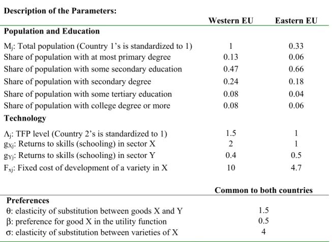
Table 2 summarizes the parametrization of the model. The parameters are either obtained from the data or calibrated to reproduce the features of the economies of Eastern and Western Europe. Workers’ skills, Z,
are measured in years of schooling. We re-scale this variable so that it ranges from 0 (no schooling) to 1 (corresponding to a Ph.D. degree, obtained with 20 years of schooling). Hence one year of schooling equals 0.05 and a secondary degree and college graduation would be aroundZ = 0.6 (=12/20) and Z= 0.8 (=16/20) respectively.13 Measuring skills with years of schooling has several advantages in this context. First, comparable schooling data for Eastern and Western European countries are available from the Barro and Lee (2001) dataset. Second, the Mincerian regression approach (very popular in the labor literature)finds that the natural logarithm of individual wages is a linear function of years of schooling. This is consistent with the wage schedule implied by our model. Third, particularly since the 1990s the returns to schooling for the highly educated in rich economies such as the U.S. and Western Europe have been larger than those for the less educated. This also matches well our characterization of the wage schedule: flatter for low values ofZ and steeper for high values ofZ. We use the schooling distributions in the year 2000 of Germany and Poland as representative of the EU-15 and of the Eastern EU members respectively as they are the largest countries in each region. Table 2 reports the share of the population in each offive schooling groups, from primary education to college graduation or more. We use those values to construct the skill distribution for Western Europe (G1(Z)) and Eastern Europe (G2(Z)).
The parametersgXjandgY j characterize the technologies employed in sectorsX andY respectively. They
can be empirically inferred from the wage schedule using equation (7). In particular, the parametergY jequals
the returns to schooling of less educated workers (to the left of Zj) while gXj equals the returns to schooling
for highly educated workers (to the right ofZj). Our calibration is based on several studies in the literature.
First, recent work by Caselli and Coleman (2006) shows that the returns to schooling at high levels of education (college) relative to those for low levels of education (primary) are particularly large in rich countries. Likewise, using data for the 1980s and 1990s Iranzo and Peri (2006) shows that the U.S. log-wage schedule has a kink around 12 years of education and that the returns to schooling are much smaller to the left of the kink than to the right. Finally, Psacharopoulos and Patrinos (2004) collect data on average returns to schooling from Mincerian regressions over several countries. Both Caselli and Coleman (2006) and Psacharopoulos and Patrinos (2004) include Germany and Poland and so we can combine those studies to calibrategY jandgXj for Western Europe
(Germany) and Eastern Europe (Poland). The values obtained are reported in Table 2.14 Consistent with the 13There are only slight differences across countries in the number of years of schooling required for those degrees.
14More precisely, we calibrategY j andgXj so that:
- The wage premia of workers with ”college completed” vs. those with ”primary completed only” equal those estimated by Caselli and Coleman (2006) for Germany and Poland.
- The yearly Mincerian return for Germany and Poland, obtained as an average of the returns to schooling of the low and highly educated (where the highly educated group is defined as those with a High School diploma or more) match those reported in Psacharopoulos and Patrinos (2004).
assumptions of the theoretical model, wefind that i) returns to skills are higher in sectorX than in sectorY
for both countries, ii) returns to skills in sectorX are larger in country 1 than in country 2, iii) returns to skills in sectorY are larger in country 2 than in country 1. These features produce the shape of the wage schedules illustrated in Figure 3. OncegY j andgXj are determined, thefixed cost parameterFXj is calibrated to ensure
that the cut-off level in autarky, ZAj, equals 12 years of schooling (secondary degree) in both countries. To complete the parameterization of the technology we need to calibrate the total factor productivity (TFP) levels for Eastern and Western Europe. Normalizing the Hicks-neutral technological parameters for Eastern Europe to 1 (i.e., Λ2= 1), we set Λ1= 1.5. Such parameters deliver an autarky equilibrium where the real per capita income of Eastern Europe is 0.39 times that of Western Europe. This value is very close to the ratio of output per worker in West Germany relative to Hungary (0.36) in the late 1980s as reported by Hall and Jones (1999) or to the ratio of output per worker in France relative to Poland (0.33). Since the data used in Hall and Jones (1999) are relative to the late 1980s we can consider those numbers as the benchmark autarky case, with very small trade and no migration between Eastern and Western Europe.
The population of Eastern Europe (adding the 10 countries that joined the EU in 2004 and in 2006) was one third the population of the Western EU countries at the moment of the entry to the EU, and since then the two blocks have followed similar demographic trends with population growth close to 0. Standardizing the population of Western Europe to 1 (M1= 1) this impliesM2= 0.33.
The rest of the parameters are assumed to be common to both regions and are reported in the lower part of Table 2. We choose the parameterθ,which measures the substitutability between goodsX andY, to match the substitutability between the workers that produce those goods (namely, low and highly educated workers). The consensus estimate for such elasticity in the literature is around 1.5 (see Katz and Murphy 1992, and Ciccone and Peri 2005). The value of σ captures the degree of substitutability between varieties of good X. This is an important parameter as the magnitude of the gains from trade of new varieties depends (inversely) on this parameter. The literature on the gains from new goods and new varieties has produced several estimates of this parameter. The value ofσ= 4 is compatible with Broda and Weinstein (2006) estimates of the elasticity of substitution between ”differentiated varieties” in 3-digit sectors. Furthermore, given the broad definition of goodX, which includes all tradeable differentiated goods and services, we choose a conservative value, in the high end of the estimated range. The parameter β is chosen to be around 0.5,15 which produces a share of expenditure inX in autarky close to 0.5 in country 1.
15As we are less confident with respect to the value of this parameter, we perform some sensitivity analyses of our results for a
5.2
Simulations: the E
ff
ects of Trade and Migration
5.2.1 Autarky and Free Trade
Our model incorporates trade and technology in a meaningful way and allows us to analyze issues not addressed before. In particular, it allows us to quantify the residual gains from reducing migration costs once there is free trade. Thus, although the main focus of the paper is to analyze the effects of freer labor mobility, it is helpful to begin with the scenario of autarky and analyze the gains from trade only. This provides valuable insights to understand the role played by trade in spreading the benefits of free labor mobility which we introduce later on. In order to obtain a clearer intuition for the results, in Tables 3 and 4 we consider a trade regime with costless trade and then in Table 5 introduce trade costs of a reasonable magnitude.
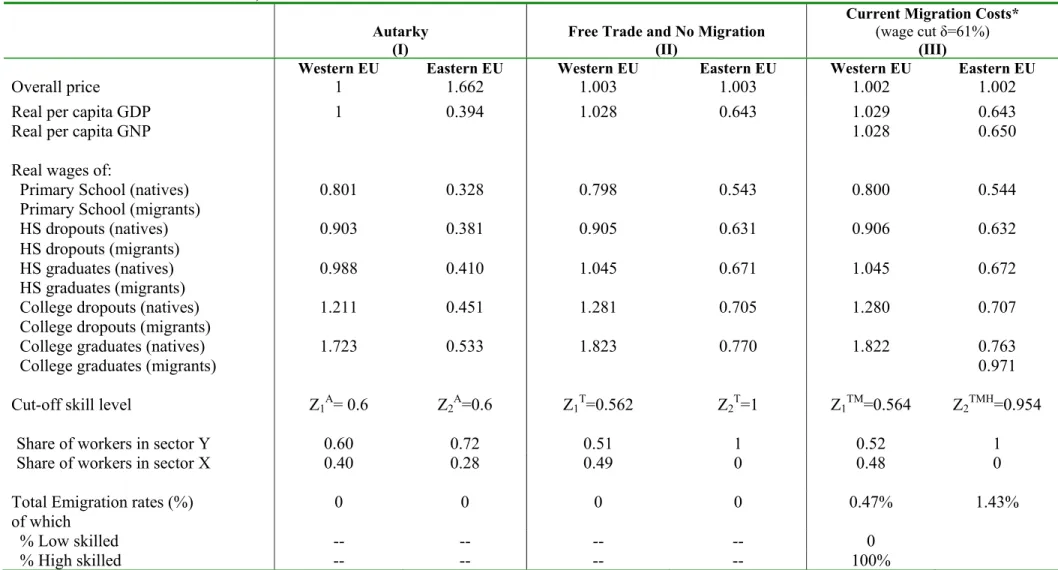
Table 3 reports the most relevant variables in the autarky equilibrium (specification I) and under free trade (specification II) for Western Europe (country 1 in our model) and Eastern Europe (country 2). For ease of comparison, we standardize the initial price level and per capita GDP in Western Europe in autarky (i.e., pre-1989) to one. Prior to 1989 per capita real GDP in Eastern Europe was 39% of the per capita income in the West. The price index was 66% higher than in the West. The price index difference in autarky is due to the East’s lower efficiency in producing goods in sectorX and the smaller range of available varieties in that sector. This is confirmed by the productive specialization of the two countries, reported towards the bottom of the table: while 40% of the workers in Western Europe work in the high tech sector, only 28% in Eastern Europe work in that sector. The productive specialization in autarky is driven by the skill composition and the technology of the two economies: Western Europe has a larger fraction of highly skilled workers (with more than high school education) and thus uses the skill-complementary technology more intensively. The rows in the mid-section of Table 3 report the real wages of workers by educational group (standardized by the per capita GDP in autarky in Western Europe) in their country of birth or, if they migrate, in their country of residence. We consider 5 educational groups: primary education, some secondary education, those with a secondary degree, some tertiary education and those with a college degree. Two things are worth noticing in the autarky equilibrium. First, workers in Eastern Europe are paid, in absolute terms, much less than in Western Europe. Even the college educated do not reach the real wage of the least educated in Western Europe. Second, in relative terms, there is a larger wage disparity in the West than in the East. The college-high school wage ratio is 1.75 in the West and only 1.3 in the East and the college-primary school wage premium is 2.15 in the West and 1.62 in the East. These wage premia reproduce the schooling premia in Germany and Poland pre-1989.
With respect to the autarky scenario the free trade equilibrium introduces three significant and intuitive changes. First, free trade ensures price equalization. This entails a substantial decrease in the overall price index for Eastern Europe, which now has access to all the good varieties produced in the West. By contrast,
the disappearance of sectorX in Eastern Europe. Given the absolute and comparative advantage of Western Europe in sector X,the opening up to trade leads to the complete specialization of Eastern Europe in sector
Y (i.e., ZT2 = 1). Western Europe still produces both goods, but its employment in sectorY is substantially reduced. Although trade changes the relative prices of goods X and Y, producing the usual Heckscher-Ohlin gains for both countries, those are small for Western Europe (the real per capita GDP increases only by 2.8%). Eastern Europe, however, benefits massively from the lower prices and the access to a larger number of varieties of goodX. Its per capita GDP increases by 63% of its initial value. This asymmetric effect is also due to the much larger size of Western Europe. The third effect of free trade is the relative benefit for the highly educated (in Western Europe) and for the less educated in Eastern Europe (Stolper-Samuelson effect). In Western Europe the college-primary school wage premium increases to 2.28 while in Easter Europe it decreases to 1.42. All in all, the real wage gains from trade for Eastern Europe dwarf the gains for Western Europe. The reader should be reminded, though, that this scenario assumes costless trade for all goods and services.
5.2.2 Free Trade and Labor Mobility
The scenario of free trade and very little labor mobility is close to the situation between Eastern and Western Europe today. Although Eastern Europe lifted the ban on emigration during the 1990s and some Western European countries received significantflows of immigrants, migrants still represent a small percentage of the total Eastern European labor force. Using the data collected by Docquier and Marfouk (2005) from national Censuses around the year 2000, we can calculate how many Eastern Europeans were in Western European countries in 2000 by educational level and then compute emigration rates (emigrants/residents of the sending country) for Eastern Europe. These rates are reported in the last row of Table 1. By educational level, one observes that the emigration rate for the highly educated is three to four times that of other groups. That is, currently the migration from Eastern Europe involves mainly the highly educated. Our model can easily explain this phenomenon: in the presence of high barriers to international labor mobility the group of highly educated workers will be the only group migrating. The last column of Table 3 presents the equilibrium when labor mobility is allowed and total migration costs (as a share of real wages) are calibrated to generate a migration rate of 14% among the highly educated (those with at least some tertiary education) and 0 for the other educational groups.16 As those with some college education are roughly 10% of the Eastern European
population, the overall emigration rate is 1.43% (reported in Table 3), and with respect to the population of the receiving economy (Western Europe) this constitutes an immigration rate of 0.47%. The value of migration costs that generates such small migration flows is δ = (δH+δB +δP) =0.61. This means that the current
hurdles to migration, inclusive of the human capital and psychological costs, are equivalent to a 61% wage cut
for the average migrant.
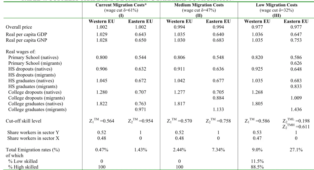
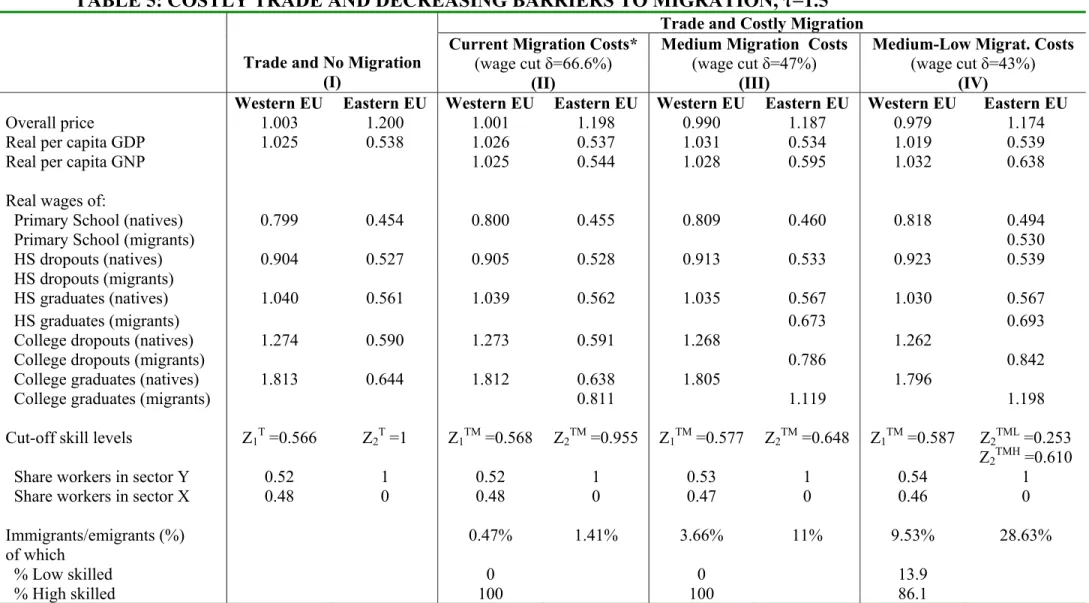
Next, we consider the effects of reductions in migration costs from their current level. The results are presented in Tables 4 and 5. For ease of comparison, the first column in Table 4 replicates specification III in Table 3; that is, it reports the per capita GDP, wages and productive specialization at the equilibrium with free trade and with the migration costs that approximate the current situation. Then we show the equilibria with intermediate migration costs (specification II) and with low migration costs (specification III). Table 5 does the same but it includes afirst specification with prohibitive migration costs and assumes costly, rather than costless, trade.
As explained in section 4.2 there are two types of migration costs that limit international migration even in the absence of legal barriers to labor mobility. Thefirst cost,δH, is the human capital loss that migrants suffer
when they move to another country. Following Borjas (1996), who empirically estimates earning losses of around 15% for Mexican immigrants to the U.S., we set δH = 0.15. The second cost, denoted δP, is a psychological
cost. Leaving loved ones and familiar places for an unknown world is obviously hard. Quantifying this cost in wage (or consumption) equivalents is a difficult task. We take the stand that these psychological costs are what constrains migration from poor to rich countries when no legal barriers to migration exist. Therefore these costs can be empirically inferred from actual migration rates in those cases with unlimited international mobility. In effect, there have been periods in history with virtually no legal restrictions on labor mobility between some countries (e.g., the period between 1880 to 1913 for the U.S.) or countries among which there are no formal barriers but still large wage differentials (e.g., the U.S. and Puerto Rico since 1945). Yet, we observe in those instances that migration falls short of what we would expect given the cross-country income differences. For example, with differences in per capita income of 2 to 1, Italian migration rates to the U.S. during the period 1880-1913 amounted to 1.3% each year, and a total of 30% over a forty-year period.17 With a per capita
income equal to one fourth that of the U.S. and full U.S. citizenship rights, Puerto Ricans had a migration rate during the 1950s and 1960s of only 0.8% each year and about 35% over thirty years. Although thesefigures are substantial, they also indicate that despite the large differences in per capita income (2 to 3 times) and no legal barriers to migration, the large majority of people do not migrate in the long run. Using a dynamic model, Klein and Ventura (2006) calibrate the psychological costs needed, on top of human capital costs of 15%, to generate an average yearly migration rate, with no barriers to labor mobility, equal to 1% per year over thefirst 25 years, which corresponds to the largest flows experienced by the countries mentioned above. They obtain a ”utility cost” that can be expressed in consumption-equivalent terms. In their preferred simulation this cost amounts to a consumption loss of about 17% of the pre-migration consumption,18 and so we useδ
P = 0.17.19 17Hatton and Williamson (2005, 2006) report similar migration rates from Ireland and Poland.
18We thank Gustavo Ventura for making available to us the average psycological cost in utility-equivalent terms implied by the
Klein and Ventura (2006) model applied to the US-Mexico case.
Hence, in the absence of legal barriers to migration, the value of total migration costsδequalsδP+δH= 0.32,
which is the value used in specification III of Table 4. Specification II features an intermediate case where we add to the previous costs some costs due to barriers to labor mobility (in particular, δB = 0.15 ) so that we
have total migrations costs ofδ= 0.47.
The effects of allowing free labor mobility are most evident when comparing specifications I and III. Several interesting effects can be observed. First, freer migration is beneficial to each country overall. The price level decreases in both countries (first row of Table 4) because highly educated Eastern Europeans move to Western Europe where they are used more efficiently and help produce a wider range of varieties of goodX.Real income increases for the average native worker in each country. To see this we should compare the per capita GNP across specifications I and III. GNP is the average income earned by natives of a country, regardless of where they reside. This value increases by 0.7% in Western Europe and by 16% in Eastern Europe going from specification I to III. The comparison of per capita GDP, however, misses most of this positive effect. On the one hand, the increased wages of emigrants from Eastern Europe is not recorded in the GDP of Eastern Europe. On the other hand, despite the increase in the wages of the natives, the inclusion of the immigrants lowers the average GDP of Western Europe due to their lower human capital relative to natives. In sum, although international migration is Pareto-improving, an analysis based on GDP per capite would be misleading.
Next we analyze the welfare effects on each educational group separately, as summarized by the real wages in Table 4. For Western Europe, the move towards freer labor mobility helps the less educated (2.5% increase in the average wages of primary school educated going from specification I to III) and hurts the most educated (about -1% change in the average wages of college educated). This is due to the skill composition of immigrants who are over-represented among the highly educated and therefore cause a negative supply side effect. As for workers in Eastern Europe, the largest gains are observed for the highly educated (who migrate).20 However, less
educated workers who remain at home are also better off. For example, college dropouts from Eastern Europe increase their net real wage (in utility terms) by 22% going from specification I to III and these gains accrue because they migrate to Western Europe. High school dropouts who remain in Eastern Europe gain 2.5% of their wage. This gain stems from the lower prices and the larger variety of goods those workers enjoy via trade. Notice also that in specification II the skill cut-offfor migrants from Eastern Europe is 0.758, which corresponds to workers with some tertiary education. That is, only workers in the top two education groups migrate, which results in a total migration rate of less than 8% of the Eastern Europe population. By contrast, specification III (with no legal migration barriers) captures the case where there is migration at the top (more than secondary
20It is important to notice that Tables 3, 4 and 5 report the real wages received by the migrants but not the
consumption-equivalent wages that would give us an idea of the utility they derive from moving. In order to translate the real wages received into utility or consumption-equivalents, to which we refer in our discussion, one needs to substract the psychological costs (estimated at 17% of the wage). Notice also that the difference in net real wages between migrants and stayers of any educational level that remains after subctracting the 17% psychological costs (see the last column of Table 4) is only due to the skill composition of those who leave (migrants) and those who stay in Eastern Europe.