MATTHIAS BURGERT, SEBASTIAN SCHMIDT
Dealing with a Liquidity Trap when
Government Debt Matters:
Optimal Time-Consistent Monetary and Fiscal Policy
INSTITUTE FOR MONETARY AND
FINANCIAL STABILITY
GOETHE UNIVERSITY FRANKFURT AM MAIN
INSTITUTE FOR MONETARY AND FINANCIAL STABILITY
GOETHE UNIVERSITY FRANKFURT HOUSE OF FINANCE
GRÜNEBURGPLATZ 1
D-60323 FRANKFURT AM MAIN
Dealing with a Liquidity Trap when
Government Debt Matters:
Optimal Time-Consistent Monetary and
Fiscal Policy
∗
Matthias Burgert
†Sebastian Schmidt
‡European Commission &
European Central Bank
IMFS, Goethe University Frankfurt
August 28, 2013
Abstract
How does the need to preserve government debt sustainability affect the optimal monetary and fiscal policy response to a liquidity trap? To provide an answer, we employ a small stochastic New Keynesian model with a zero bound on nominal inter-est rates and characterize optimal time-consistent stabilization policies. We focus on two policy tools, the short-term nominal interest rate and debt-financed government spending. The optimal policy response to a liquidity trap critically depends on the prevailing debt burden. While the optimal amount of government spending is decreas-ing in the level of outstanddecreas-ing government debt, future monetary policy is becomdecreas-ing more accommodative, triggering a change in private sector expectations that helps to dampen the fall in output and inflation at the outset of the liquidity trap.
JEL Classification: E31, E52, E62, E63, D11
Keywords: Monetary Policy, Fiscal Policy, Deficit spending, Discretion, Zero nominal interest rate bound, New Keynesian model
∗The views expressed in this paper are those of the authors and do not necessarily represent those of the
European Commission or the European Central Bank.
†European Commission, DG Economic and Financial Affairs, Rue de la Loi 170, B-1000 Brussels, Belgium.
Email: matthias.burgert@ec.europa.eu
‡European Central Bank, Monetary Policy Research Division, Kaiserstr 29, 60311 Frankfurt, Germany.
1
Introduction
New Keynesian characterizations of optimal time-consistent monetary and fiscal policies in a liquidity trap typically omit government debt from the analysis, assuming that government purchases are financed by lump-sum taxes (e.g. Werning, 2011; Schmidt, 2012; Nakata, 2013). At the same time, the enormous increase in government debt-to-GDP ratios in the course of the recent global financial crisis in major industrialized countries raises important questions about the appropriate stance of monetary and fiscal policy. Should policymakers adhere to fiscal stimulus in the face of a zero lower bound event if the level of government debt is already above its long-run target? How does the need to ensure debt sustainability act upon the effectiveness of monetary policy? In terms of model-based characterizations of optimal policies at the zero lower bound, is the conventional omission of government debt innocuous or do our normative prescriptions change when we account for the fact that lump-sum taxes in general do not adjust one-to-one with other fiscal variables?
We address these questions in a stylized stochastic New Keynesian model with a zero bound on nominal interest rates that accounts for government debt in the form of non-state-contingent, one-period, nominal government bonds as a means of financing government spending. The benevolent government controls the short-term nominal interest rate and the level of government spending, and decides about the supply of government bonds. Hence, in the economy that we consider the central bank and the fiscal authority coordinate their policy measures. We focus on time-consistent policy regimes since it is the absence of a commitment device that renders the zero lower bound detrimental for stabilization policy.1
Households appreciate private consumption as well as the provision of public goods and dis-like labor. For the ease of exposition, we assign only a very limited role to tax policy in our baseline model. First, private consumption and household labor income are taxed at constant rates, providing revenues to the government. Second, lump-sum taxes are used to finance a constant wage subsidy to ensure that the distortions arising from monopolistic competition in the goods market and from the other taxes are eliminated in the non-stochastic steady state. However, we also present results for the case where the policymaker sets the labor tax rate optimally. Economic uncertainty arises from the presence of a demand shock.
We solve the model using a projection method and then explore how government debt af-fects optimal policies and stabilization outcomes when the zero bound on nominal interest rates becomes occasionally binding. The presence of government debt makes the optimal time-consistent policy history dependent, that is, the future path of the policy instruments
1For a characterization of optimal monetary policy under commitment see e.g. Eggertsson and Woodford
depends on today’s level of government debt. We show, that, first, for a given realization of the demand shock, government spending is decreasing in the level of outstanding gov-ernment debt, i.e. the fiscal stance becomes more contractionary when govgov-ernment debt rises. Second, as long as the zero lower bound is not binding, the nominal interest rate is decreasing in the level of government debt. Real interest rates keep declining as a function of the debt level even if the zero bound on the nominal rate is binding, i.e. the monetary policy stance becomes more expansionary the higher the government debt burden. Third, output and inflation are both increasing in beginning-of-period debt, irrespective of whether the zero bound is binding or not.
How the economy responds to a liquidity trap thus critically depends on the prevailing gov-ernment debt level. If, for instance, the level of outstanding govgov-ernment debt is high relative to its steady state, then the optimal policy mix will prescribe at most a small government spending stimulus, followed by a spending reversal, and a prolonged period of expansionary monetary policy. The policymaker creates valid expectations of a subsequent boom in in-flation and output that help to dampen the economic turmoil at the outset of the liquidity trap. If, on the other hand, the public debt level is low relative to its steady state, gov-ernment spending is used forcefully to stimulate aggregate demand, when the economy falls into a liquidity trap. In this situation, however, the zero bound episode is not followed by a boom in output and inflation. Absent the expansionary expectations effects of the high debt scenario, the low debt scenario exhibits larger drops in output and inflation.
The ability to issue government debt allows the policymaker to influence private sector expec-tations without engaging in time-inconsistent policies. As emphasized by Krugman (1998) and Eggertsson and Woodford (2003), during zero lower bound episodes, expectations about future output and inflation can have considerable effects on contemporaneous stabilization outcomes. We demonstrate the powerfulness of government debt-induced history dependence by comparing optimal discretionary policies and stabilization outcomes for a liquidity trap scenario in our baseline economy with those in the conventional model setup that features zero government debt and lump-sum taxes that adjust each period to balance the govern-ment budget.
Our paper is closely related to work by Eggertsson (2006), who first showed that the accu-mulation of government debt allows a discretionary policymaker to influence expectations about the path of monetary policy after the liquidity trap. Our paper differs from this earlier work in several respects. First, the fiscal instrument considered by Eggertsson is a lump-sum tax. In his model, the policymaker lowers lump-sum taxes when the zero bound is binding in order to increase government debt. Tax collection costs make it credible that the increase in government debt will not be solely undone by future tax increases. There is no immediate
trade-off for fiscal policy in a liquidity trap between stimulating the economy and stabilizing government debt. In our paper, the liquidity trap shock reduces the tax base, which may force the policymaker to tighten fiscal policy while the zero lower bound is binding. Second, in Eggertsson’s model, the economy starts in a liquidity trap state and returns to the nor-mal state with a constant probability in each subsequent period, where it will stay forever. Instead, in our model, the zero nominal interest rate bound is an occasionally binding con-straint. We show that the outstanding amount of government debt prior to the zero bound event critically affects stabilization policies and outcomes in the liquidity trap. For instance, if government debt is low relative to its steady state, then the policymaker may refrain from lowering the nominal interest rate all the way to zero, which exacerbates the fall in output and inflation. Finally, we show, that, unlike in Eggertsson (2006), the optimal discretionary policy is not necessarily associated with a transitory boom in output and inflation after the liquidity trap.
The paper can also be related to studies that investigate optimal monetary and fiscal policy under commitment at the zero lower bound and account for the presence of government debt. Eggertsson and Woodford (2006) determine the optimal nominal interest rate and tax pol-icy mix. Nakata (2011) characterizes the optimal plan for distortionary taxes, government spending and the short-term nominal interest rate.
Finally, several studies have characterized optimal monetary and fiscal policy in New Key-nesian models that account for the presence of government debt but abstract from the zero bound on nominal interest rates. Wren-Lewis and Leith (2007) and Vines and Stehn (2007) characterize the optimal policy mix under discretion, whereas Schmitt-Grohe and Uribe (2004) and Adam (2011) analyse optimal commitment policies.
The remainder of the paper is organized as follows. Section 2 presents the model economy. Section 3 specifies the policy problem. Section 4 presents numerical results. Finally, Section 5 concludes.
2
The model
We consider a small monetary business cycle model with nominal rigidities and monopolistic competition. The economy is inhabited by a continuum of identical households of measure one, a final good producer, a continuum of intermediate-goods-producing firms of measure one, and a benevolent policymaker. Following Woodford (2003), the model is treated as a cashless limiting economy. Time is discrete and indexed by t.
2.1
Households and firms
The representative household obtains utility from a private consumption good Ct and the
provision of a public consumption good Gt, and dislikes labor Nt(i),∀i ∈ [0,1]. Expected
lifetime utility of the household reads E0 ∞ X t=0 βt u(Ct) +g(Gt)− Z 1 0 ν(Nt(i))di , (1)
where Et is the rational expectations operator conditional on information in period t and
β ∈ (0,1) is the discount factor. The functions u(·) and g(·) are increasing and concave in their arguments, andν(·) is increasing and convex in its argument.
The household enters period t with a degenerate portfolio of non-state-contingent, one-period, nominal government bonds Bt−1, paying the household Bt−1/Pt units in terms
of the final consumption good. For simplicity, we assume that one-period government bonds are the only assets traded in the economy. The household supplies Nt(i) units
of labor to the producer of intermediate good i and earns total after-tax labor income R1
0 1−τ
NW
t(i)Nt(i)di, where Wt(i) denotes the nominal wage rate payed by firm i
and τN is a constant labor income tax rate. Furthermore, the household receives dividend
paymentsPtΨtfrom intermediate-goods-producing firms, which are owned by the household.
The household uses her labor income, dividend income and the government’s debt repay-ment to finance purchases of the private consumption good at price 1 +τCP
t whereτC is
a constant consumption tax rate, to pay lump-sum taxesPtTt, and to buy newly issued
gov-ernment bonds at price 1/(1 +it), whereit ≥0 is the one-period, riskless, nominal interest
rate. The flow budget constraint reads 1 +τCPtCt+ Bt 1 +it ≤ Z 1 0 1−τNWt(i)Nt(i)di+Bt−1−PtTt+ Ψt. (2)
The representative household maximizes her expected lifetime utility (1) by choosing state-contingent plans {Ct >0, Nt(i)>0, Bt}∞t=0 subject to (2) and a no-Ponzi game condition
lim j→∞Et t+j Y k=0 1 1 +ik ! Bt+j ! ≥0.
The final consumption good is produced under perfect competition using the following technology Yt = Z 1 0 Yt(i) θ−1 θ di θ θ−1 ,
where θ > 1 and Yt(i) denotes the intermediate input i. Total demand for the final good
consists of household and government demand
Yt=Ct+Gt.
The market for intermediate goods features monopolistic competition. Expenditure mini-mization by the producer of the final good results in the following demand for intermediate good i Yt(i) = Pt(i) Pt −θ Yt, (3)
wherePt(i) denotes the price charged by firmi andPt=
R1 0 Pt(i) 1−θ di 1 1−θ represents the price for the final consumption good. Intermediate goods are produced using labor
Yt(i) = Nt(i).
There is no capital. Intermediate-goods firms face price rigidities `a la Calvo (1983). In each period, a fraction 1−α of firms is allowed to change prices, whereas the remaining fraction
α ∈ (0,1) of firms keep their price constant at previous period’s level. Each intermediate goods firm i that is allowed to reset prices in period t maximizes its expected discounted profits: max Pt(i) ∞ X j=0 EtQt,t+jαjYt+j(i) [Pt(i)−(1−τ)Wt+j(i)],
subject to (3). The parameter τ denotes a constant employment subsidy that eliminates the distortions arising from monopolistic competition and distortionary taxes in the non-stochastic steady state andQt,t+j =βj U
′(C
t+j)/Pt+j
U′(Ct)/Pt is the stochastic discount factor between period t and t+j.
2.2
The government
The government issues non-state-contingent, one-period, nominal government bonds and levies lump-sum taxes, labor income taxes and consumption taxes to finance public spending and the provision of a constant wage subsidy τ, and to service the debt incurred from the previous period. We assume that the government can credibly promise to repay its debt each period. The flow budget constraint reads
PtGt+τ Z 1 0 Wt(i)Nt(i)di+Bt−1 = Bt 1 +it +PtTt+τCPtCt+τN Z 1 0 Wt(i)Nt(i)di.
In real terms Gt+τ Z 1 0 wt(i)Nt(i)di+bt−1π−t1 = bt 1 +it +Tt+τCCt+τN Z 1 0 wt(i)Nt(i)di, where bt =Bt/Pt, πt=Pt/Pt−1, and wt(i) =Wt(i)/Pt.
Assumption 1 Lump-sum taxes are used to finance the wage subsidy. Beyond that, a
con-stant amount of (possibly negative) lump-sum tax revenues TG is available to finance
gov-ernment spending and to service public debt
Tt=TG+τ
Z 1 0
wt(i)Nt(i)di.
We can then simplify the budget constraint
Gt+bt−1π−t1 = bt 1 +it +TG+τCCt+τN Z 1 0 wt(i)Nt(i)di. (4)
2.3
Equilibrium
An equilibrium consists of paths{Ct, Nt(i), Yt(i), Yt, Bt, Gt, it, Pt(i), Pt, Wt(i)}∞t=0, given an
initial level of government debt B−1 and identical initial goods prices P−1(i)∀i, such that
(i) {Ct, Nt(i), Bt}∞t=0 solves the household optimization problem given prices and policies,
(ii){Pt(i)}∞t=0 solves the optimization problem of producer i, (iii) the government budget
constraint and the zero lower bound on the nominal interest rate it ≥ 0 are satisfied, and
(iv) the goods market, the labor market, and the government bond market clear.
2.4
Log-linear approximation
The optimization problems of households and firms are standard, we therefore refrain from presenting optimality conditions and directly continue with a log-linear approximation of the resulting behavioral constraints around the non-stochastic steady state with zero inflation
ˆ πt = κ ˆ Yt−Γ ˆGt +βEtπˆt+1 (5) ˆ Yt = Gˆt+ EtYˆt+1−EtGˆt+1− 1 σ(it−Etπˆt+1−r ∗) +d t. (6)
Hat variables denote percentage deviations from the deterministic steady state. ˆπt is the
inflation rate between period t−1 and t, ˆYt represents real output, and ˆGt denotes
gov-ernment spending expressed as a share of steady state output. The parameter r∗ = 1
denotes the steady state real interest rate, and σ ≡ −uu′′′((CC))Y represents the elasticity of the marginal utility of private consumption with respect to total output in the steady state. The parameters κ and Γ are functions of structural parameters
κ= (1−α)(1−αβ)
α(1 +ηθ) (σ+η), Γ =
σ
σ+η,
where η > 0 denotes the inverse of the labor supply elasticity, α ∈ (0,1) represents the share of firms that are unable to change their price in a given period, and θ >1 is the price elasticity of demand for intermediate goods. We assume that the economy is subject to an exogenous demand shock dt that follows a stationary autoregressive process
dt=ρdt−1+ǫt, (7)
where ǫt is a i.i.d. N(0, σǫ2) innovation, and ρ∈[0,1).
Finally, the log-linearized government budget constraint (4) reads2
ˆ bt = 1 β ( ˆ bt−1− b Y πˆt+ 1 +τC + 1 +τ C 1−τNτ Nσ ˆ Gt− τC + 1 +τ C 1−τNτ N(1 +σ+η) ˆ Yt ) +b Y (it−r ∗), (8) where ˆbt = bt−Yb.
3
The policy problem
The benevolent policymaker aims to maximize expected lifetime utility (1) of the representa-tive household. We conduct a linear-quadratic approximation to household welfare to obtain a quadratic policy objective function.3 Each period t, the policymaker minimizes the loss
function from period t onwards, taking the decision rules of the private sector and future governments as given. We focus on stationary Markov-perfect equilibria, where the vector of state variables consists of the demand shock and the beginning-of-period government debt
2In the deterministic steady state 1 +τCG
Y + (1−β) b Y = TG Y +τ C+ 1+τC 1−τNτN.
3See Schmidt (2012) for the details of the derivation. We ensure that the non-stochastic steady state of the
flexible-price equilibrium is efficient by choosing the constant wage subsidy such that it offsets the distortions arising from monopolistic competition and taxes in the non-stochastic steady state,τ= 1−θ−1
θ
1−τN
level, st= (dt,ˆbt−1). The Bellman equation reads V(st) = min {πˆt,Yˆt,Gˆt,it,ˆbt} " 1 2 ˆ πt2+λYˆt−Γ ˆGt 2 +λGGˆ2t +βEtV(st+1) # subject to ˆ πt = βEtπˆ(st+1) +κ ˆ Yt−Γ ˆGt ˆ Yt = Gˆt+ EtYˆ(st+1)−EtGˆ(st+1)− 1 σ(it−Etπˆ(st+1)−r ∗) +d t ˆ bt = 1 β ( ˆbt−1− b Y πˆt+ 1 +τC+ 1 +τ C 1−τNτ Nσ ˆ Gt− τC+ 1 +τ C 1−τNτ N (1 +σ+η) ˆ Yt ) +b Y (it−r ∗) it ≥ 0,
and the law of motion for the demand shock (7). The functions ˆπ(st+1), ˆY(st+1) and ˆG(st+1)
represent the inflation rate, output and government spending that the policymaker expects to be realized in period t+ 1 in equilibrium, contingent on the realization of the demand shock dt+1. The relative weights λ and λG in the policymaker’s objective function depend
on the structural parameters
λ = κ θ, λG=λΓ 1−Γ + ω σ ,
where ω ≡ −gg′′′((GG))Y is the elasticity of the marginal utility of public consumption with respect to total output.
The first-order conditions read
λGGˆt+ 1 β + (1−Γ) b Y σ+ 1 β (1−Γ)τ C − β1Γ1 +τ C 1−τNτ N Φbt−(1−Γ) Φzlbt = 0 (9) EtΦb(st+1)−Ω1tΦtb+ Ω2tπˆt−Ω3tΦzlbt = 0(10) Φzlbt it = 0(11) Φzlbt ≥ 0(12) it ≥ 0(13)
as well as the New Keynesian Phillips curve, the dynamic IS curve and the government budget constraint, where
Φzlb t ≡ b Y σ+ κ β + 1 β τC + 1 +τC 1−τNτ N(1 +σ+η) Φb t− κπˆt+λ ˆ Yt−Γ ˆGt Ω1t ≡ 1−σ b Y ∂EtYˆ(st+1) ∂ˆbt − ∂EtGˆ(st+1) ∂ˆbt ! Ω2t ≡ β ∂Etπˆ(st+1) ∂ˆbt Ω3t ≡ ∂EtYˆ(st+1) ∂ˆbt −∂EtGˆ(st+1) ∂ˆbt + 1 σ ∂Etπˆ(st+1) ∂ˆbt . The variable Φb
t is the multiplier associated with the government budget constraint and
Φzlb
t represents the (normalized) multiplier associated with the zero lower bound constraint.
Solving condition (9) for government spending, we get ˆ Gt= 1 λG (1−Γ) Φzlbt − 1 β + (1−Γ) b Y σ+ 1 β (1−Γ)τ C − β1Γ1 +τ C 1−τNτ N Φbt . (14)
Assumption 2 The parameters satisfy 1 + Γ +τCτN ≤1 + (1−Γ)τC.
This assumption is sufficient to ensure that the coefficient on Φb
t in (14) is negative.
Note, first, that the second term in equation (14) would vanish if we assumed that government spending is financed by lump-sum taxes. In this case, government spending would only be used as a stabilization tool if the zero lower bound were binding, and the fiscal policy stance during zero bound events would be unequivocally expansionary, see Schmidt (2012).
In the model with government debt, however, public spending may have to deviate from its steady state level even if the economy is away from the zero lower bound so that Φzlb
t = 0.
Intuitively, whenever monetary policy is unable to stabilize government debt as well as inflation and output simultaneously, government spending will be used as an additional stabilization tool.
Furthermore, from (14) it is not clear whether fiscal policy in a liquidity trap should be expansionary, ˆGt > 0, or contractionary, ˆGt < 0. Specifically, if Φbt > 0, the zero bound
multiplier and the government budget constraint multiplier have opposite implications for the sign of the fiscal policy response. As we will show below, stabilization outcomes and policies in a liquidity trap critically depend on the amount of outstanding government debt when hitting the zero bound.
4
Numerical results
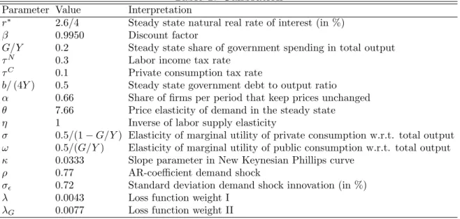
In this section, we characterize the optimal time-consistent policy mix numerically. The policy functions are approximated using a projection method with finite elements. The procedure is described in the Appendix. The baseline calibration is presented in Table 1, where the period length is one quarter. The steady state real interest rate and the law of motion of the demand shock are calibrated based on U.S. data for 1983 to 2010. We set the ratio of government spending to total output in the deterministic steady state equal to 0.2. The labor income tax rate is set to 0.3 and the consumption tax rate to 0.1, as in Denes, Eggertsson, and Gilbukh (2013). In the baseline, the steady state government debt to annualized output ratio is set to 0.5 but we also consider lower and higher values in the sensitivity analysis. All other structural parameters assume standard values from the literature.
Table 1: Calibration
Parameter Value Interpretation
r∗ 2.6/4 Steady state natural real rate of interest (in %)
β 0.9950 Discount factor
G/Y 0.2 Steady state share of government spending in total output
τN 0.3 Labor income tax rate
τC 0.1 Private consumption tax rate
b/(4Y) 0.5 Steady state government debt to output ratio
α 0.66 Share of firms per period that keep prices unchanged
θ 7.66 Price elasticity of demand in the steady state
η 1 Inverse of labor supply elasticity
σ 0.5/(1−G/Y) Elasticity of marginal utility of private consumption w.r.t. total output
ω 0.5/(G/Y) Elasticity of marginal utility of public consumption w.r.t. total output
κ 0.0333 Slope parameter in New Keynesian Phillips curve
ρ 0.77 AR-coefficient demand shock
σǫ 0.72 Standard deviation demand shock innovation (in %)
λ 0.0043 Loss function weight I
λG 0.0077 Loss function weight II
4.1
Optimal time-consistent policy in a liquidity trap
We begin our discussion of the optimal time-consistent policy with an experiment where the occurrence of a large negative demand shock pushes the economy for several quarters into a liquidity trap. Figure 1 shows impulse responses of output, inflation, government spending, the nominal interest rate, government debt and the real interest rate to a negative demand shock of −3 unconditional standard deviations when the economy is initially in the risky steady state. The realized paths in the absence of any further shocks are represented by solid lines, the expected paths as of period 0 are represented by dashed lines and blue-shaded
areas represent confidence intervals. The demand shock materializing in period 0 drives the Figure 1: Impulse responses to a negative demand shock
0 2 4 6 8 10 12 −4 −2 0 2 Output 0 2 4 6 8 10 12 −1 −0.5 0 0.5 1 Inflation rate 0 2 4 6 8 10 12 −2 −1 0 1 2 3 Government spending 0 2 4 6 8 10 12 0 2 4 6
Nominal interest rate
0 2 4 6 8 10 12 −2 0 2 4 quarters Government debt 0 2 4 6 8 10 12 −6 −4 −2 0 2 4 6 quarters Real interest rate
Notes: Impulse responses to a−3 unconditional standard deviation demand shock for the baseline calibration. Realized path (solid line), path expected in period 0 (dashed line), 50%, 75% and 90% confidence intervals (shaded areas). Inflation and interest rates are expressed in annualized terms. Government debt is expressed as a share of annualized steady state output, government spending is expressed as a share of steady state output.
natural real rate of interest r∗
t =r∗+σdt into negative territory and forces the policymaker
to lower the short-term nominal interest rate to zero where it stays for several periods. The economy starts to contract, both output and inflation drop below their target levels, and the reduction in the tax base leads to an increase in government debt. The fiscal policy response is first expansionary, contributing to the accumulation of government debt, but turns slightly contractionary before the zero bound episode ends. Figure 2 decomposes the response of government spending into the response of the zero lower bound multiplier component (dashed line) and the response of the budget constraint multiplier component (dashed-dotted line)
as in equation (14). Initially, both components exhibit a positive sign, which means that Figure 2: Decomposition of government spending response
0 2 4 6 8 10 12 −0.5 0 0.5 1 1.5 2 quarters Government spending ZLB component BC component
Notes: Impulse responses of government spending (solid line), the zero lower bound
mul-tiplier component 1−Γ
λGΦ
zlb
t (dashed line) and the budget constraint multiplier component
−λ1G 1 β + (1−Γ) b Yσ+ 1 β(1−Γ)τ C −β1Γ 1+τC 1−τNτ NΦb
t (dashed-dotted line) to a demand shock of
−3 unconditional standard deviations.
Φzlb
t > 0 and Φbt <0. The negative budget constraint multiplier implies that it would have
been desirable from a welfare perspective if the government had entered the period with a somewhat higher debt level. However, in subsequent periods when the government debt burden has become more elevated the budget constraint multiplier component switches signs, turning from positive to negative, and government spending declines below its pre-shock level. Coming back to Figure 1, while the increased debt burden narrows the room for expansionary fiscal policy, it facilitates the implementation of an expansionary monetary policy stimulus. Once the natural real rate has reentered positive territory, the nominal interest rate remains transitorily below the level that would be warranted by output and inflation stabilization considerations alone in order to contribute to the stabilization of government debt. As a consequence, the economy experiences a small boom in output and inflation. Importantly, private agents attach positive probabilities to positive future realizations of output and inflation and (correctly) expect both variables to move temporarily above their target levels,
which attenuates the drop at the outset of the zero bound event.
4.2
Equilibrium responses to government debt
To provide a more general characterization of the optimal time-consistent policy and how it is affected by the level of outstanding government debt, Figure 3 displays equilibrium responses to the beginning-of-period government debt level. We consider two alternative realizations of the demand shock, d = 0 (solid line) and d = −3 unconditional standard deviations (dashed line). For both values of d, the optimal amount of government spending
Figure 3: Equilibrium responses to previous period’s government debt
−2 0 2 4 −6 −4 −2 0 2 Output −2 0 2 4 −2 −1 0 1 Inflation −2 0 2 4 −2 −1 0 1 2 3 Government spending −2 0 2 4 0 2 4 6 8
Nominal interest rate
−2 0 2 4 −2 0 2 4 Government debt
Lagged debt level
−2 0 2 4 0 2 4 6 8
Real interest rate
Lagged debt level
d=0 d=-3√σǫ
1−ρ2
Notes: Equilibrium responses to the beginning-of-period government debt level. The demand shock is either set equal to zero (solid line) or to−3 unconditional standard deviations (dashed line). Inflation and interest rates are expressed in annualized terms. Government debt is expressed as a share of annualized steady state output, government spending is expressed as a share of steady state output.
is decreasing in the public debt burden. Thus, if the beginning-of-period level of government debt is high, the fiscal policy response to a liquidity trap becomes considerably muted. At the same time, inflation and output are both increasing in the level of outstanding public
debt. Monetary policy turns out to be crucial to understand this result. The higher the level of government debt incurred from the previous period the lower the nominal interest rate, as long as the zero lower bound is not binding. In other words, under the optimal policy mix, monetary policy bears part of the responsibility to stabilize government debt. Moreover, the real interest rate keeps decreasing in the level of outstanding debt even if the zero nominal interest rate bound is binding, reflecting the positive effect of government debt on expected future inflation. Intuitively, if monetary policy is unable to lower the current nominal interest rate further, because the zero bound is binding, future monetary policy will have to stabilize government debt, thereby stimulating future output and inflation. If, on the contrary, the level of outstanding government debt is low relative to the steady state, when a large negative demand shock hits the economy, then the policymaker may even refrain from lowering the nominal interest rate immediately all the way to zero. While the government spending stimulus in such states is particularly large, the decline in output and inflation is more pronounced than in states with higher levels of outstanding government debt.
4.3
Comparison to the case without government debt
In the previous parts, we have characterized the optimal time-consistent policy mix in the presence of government debt. We now compare this optimal policy mix to the one in an economy where government debt is zero, distortionary taxes are zero as well, and lump-sum taxes are free to adjust each period to balance the budget. Figures 4 and 5 show impulse responses to a negative demand shock for the two economies.4 The policymaker in the model
without government debt engages in a more pronounced fiscal stimulus and implements a lower nominal interest rate path than his counterpart in the economy with government debt. Nevertheless, the drop in output and inflation turns out to be considerably larger. The comparison shows how powerful history dependence is in affecting stabilization outcomes by shaping private sector expectations. In the economy without government debt, agents anticipate that the policymaker will never allow inflation to rise above target, which is reflected in the corresponding confidence intervals. In contrast, agents in the model with government debt anticipate that if current conditions got worse so that government debt increased,futuremonetary policy would respond to today’s economic conditions by becoming more accommodative than would be warranted by future inflation and output gap dynamics alone. Hence, they attach positive probabilities to above-target future output and inflation, and the expected real interest rate path lies below its counterpart in the model without
4For the comparison we setσ= 3−1/(1−G/Y) andω= 3−1/(G/Y), since the model without government
debt cannot be solved for the baseline calibration. The effect of this change in parameter values is addressed in the sensitivity analysis.
Figure 4: Impulse responses with and without government debt 0 2 4 6 8 10 12 −1 0 1 2 3 4 Government spending
With government debt
0 2 4 6 8 10 12 0
2 4 6
Nominal interest rate
0 2 4 6 8 10 12 −4 −2 0 2 4 6
Real interest rate
quarters 0 2 4 6 8 10 12 −1 0 1 2 3 4
Without government debt
0 2 4 6 8 10 12 0 2 4 6 0 2 4 6 8 10 12 −4 −2 0 2 4 6 quarters
Notes: Impulse responses to a −3 unconditional standard deviation demand shock for the economy with positive government debt (left) and for an economy with zero government debt (right). Except for σ = 3−1/(1−G/Y) and ω = 3−1/(G/Y), the baseline calibration is used. Inflation and interest rates are
expressed in annualized terms. Government debt is expressed as a share of annualized steady state output, government spending is expressed as a share of steady state output.
government debt.
4.4
Sensitivity analysis
In this section, we investigate the sensitivity of results to preference parameters, the degree of price stickiness and the choice of the steady state debt-to-output ratio.
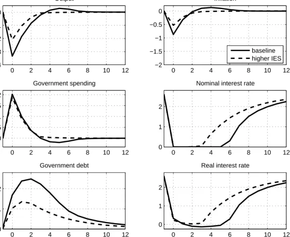
First, we consider how the intertemporal elasticity of substitution in private and public spending affects stabilization policies and outcomes in a liquidity trap. Figure 6 shows im-pulse responses for the baseline calibration and for the case of somewhat higher intertemporal elasticities, σ= 3−1/(1−G/Y) andω = 3−1/(G/Y). The change inσ increases the interest
Figure 5: Impulse responses with and without government debt 0 2 4 6 8 10 12 −4 −3 −2 −1 0 1 Output
With government debt
0 2 4 6 8 10 12 −1.5 −1 −0.5 0 0.5 Inflation rate 0 2 4 6 8 10 12 −1 0 1 2 3 Government debt quarters 0 2 4 6 8 10 12 −4 −3 −2 −1 0 1
Without government debt
0 2 4 6 8 10 12 −1.5 −1 −0.5 0 0.5 0 2 4 6 8 10 12 −1 0 1 2 3 quarters
Notes: Impulse responses to a −3 unconditional standard deviation demand shock for the economy with positive government debt (left) and for an economy with zero government debt (right). Except for σ = 3−1/(1−G/Y) and ω = 3−1/(G/Y), the baseline calibration is used. Inflation and interest rates are
expressed in annualized terms. Government debt is expressed as a share of annualized steady state output, government spending is expressed as a share of steady state output.
and inflation than under the baseline calibration. Consequently, we observe smaller declines of output and inflation. Government debt increases by less so that no fiscal retrenchment is necessary to stabilize the economy, and output and inflation do not overshoot their target levels.
Figure 7 shows impulse responses for two alternative degrees of price stickiness, the baseline case with a Calvo parameter ofα = 0.66 (solid line) and an alternative case with more price rigidities, α = 0.75 (dashed line). The policy responses for the two calibrations are very similar. In case of a higher degree of price stickiness, however, inflation is less responsive to variations in current real activity so that the initial drop in the inflation rate as well as the subsequent boom are more muted than under the baseline calibration.
Figure 6: Impulse responses for alternative intertemporal elasticities of substitution 0 2 4 6 8 10 12 −4 −3 −2 −1 0 Output 0 2 4 6 8 10 12 −2 −1.5 −1 −0.5 0 Inflation baseline higher IES 0 2 4 6 8 10 12 0 0.5 1 1.5 2 Government spending 0 2 4 6 8 10 12 0 1 2
Nominal interest rate
0 2 4 6 8 10 12 0 1 2 Government debt quarters 0 2 4 6 8 10 12 0 1 2
Real interest rate
quarters
Notes: Impulse responses to a−3 unconditional standard deviation demand shock for the baseline calibration (solid line) and in case of higher intertemporal elasticities of substitution (dashed line). Inflation and interest rates are expressed in annualized terms. Government debt is expressed as a share of annualized steady state output, government spending is expressed as a share of steady state output.
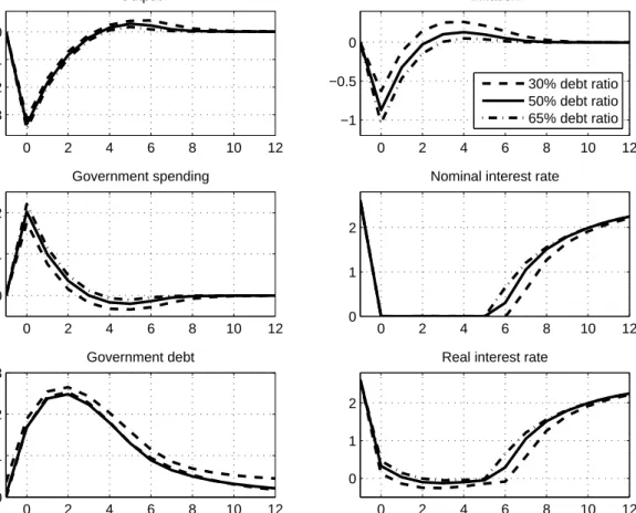
lower (30%) and a higher (65%) steady state government debt-to-output ratio. The higher the steady state debt ratio, the more leverage do changes in the nominal interest rate have over the government’s interest rate payments. Hence, in case of the low steady state debt ratio, monetary policy is less effective in stabilizing government debt and therefore keeps nominal interest rates low for longer than in the baseline case. At the same time, fiscal policy is less expansionary and engages in a stronger subsequent retrenchment in order to stabilize government debt and to mitigate the boom in future output and inflation. Never-theless, output and inflation decline less on impact than in the baseline case. Conversely, in the case of the high steady state government debt-to-output ratio the policymaker imple-ments a bigger spending stimulus but keeps monetary policy less accommodative, resulting in somewhat larger drops in output and inflation.
Figure 7: Impulse responses for alternative degrees of price stickiness 0 2 4 6 8 10 12 −4 −3 −2 −1 0 Output 0 2 4 6 8 10 12 −1 −0.5 0 Inflation α=0.66 α=0.75 0 2 4 6 8 10 12 0 0.5 1 1.5 2 Government spending 0 2 4 6 8 10 12 0 1 2
Nominal interest rate
0 2 4 6 8 10 12 0 1 2 Government debt quarters 0 2 4 6 8 10 12 0 1 2
Real interest rate
quarters
Notes: Impulse responses to a−3 unconditional standard deviation demand shock for the baseline calibration (solid line) and for a higher degree of price stickiness ofα= 0.75(dashed line). Inflation and interest rates are expressed in annualized terms. Government debt is expressed as a share of annualized steady state output, government spending is expressed as a share of steady state output.
4.5
Labor income tax as additional policy instrument
In this section, we relax the assumption of a constant labor income tax rate, endowing the policymaker with an additional fiscal instrument. The modified Bellman equation then reads as follows: V(st) = min {πˆt,Yˆt,Gˆt,it,ˆbt,τˆtN} 1 2 ˆ πt2+λYˆt−Γ ˆGt 2 +λGGˆ2t +βEtV(st+1)
Figure 8: Impulse responses for alternative steady state government debt ratios 0 2 4 6 8 10 12 −3 −2 −1 0 Output 0 2 4 6 8 10 12 −1 −0.5 0 Inflation 30% debt ratio 50% debt ratio 65% debt ratio 0 2 4 6 8 10 12 0 1 2 Government spending 0 2 4 6 8 10 12 0 1 2
Nominal interest rate
0 2 4 6 8 10 12 0 1 2 3 Government debt quarters 0 2 4 6 8 10 12 0 1 2
Real interest rate
quarters
Notes: Impulse responses to a −3 unconditional standard deviation demand shock in case of steady state debt-to-output ratios of 30% (dashed lines), 50% (solid lines) and 65% (dashed-dotted lines). Inflation and interest rates are expressed in annualized terms. Government debt is expressed as a share of annualized steady state output, government spending is expressed as a share of steady state output.
subject to ˆ πt = βEtˆπ(st+1) +κ ˆ Yt−Γ ˆGt+ (σ+η)−1 1−τN τˆ N t ˆ Yt = Gˆt+ EtYˆ(st+1)−EtGˆ(st+1)− 1 σ (it−Etπˆ(st+1)−r ∗) +d t ˆbt = 1 β ˆbt−1− b Y πˆt+ 1 +τC+ 1 +τ C 1−τNτ Nσ ˆ Gt− τC+ 1 +τ C 1−τNτ N(1 +σ+η) ˆ Yt − 1 +τ C (1−τN)2τˆ N t ! + b Y (it−r ∗) it ≥ 0,
and the law of motion for the demand shock (7), where ˆτN
t = τtN −τN. All parameters
are defined as before. The first-order optimality conditions are provided in the Appendix. Figure 9 displays impulse responses to a negative demand shock that drives the economy into a liquidity trap5. Upon occurrence of the shock, the labor income tax rate is initially
Figure 9: Impulse responses - variable labor income tax rate
0 2 4 6 8 10 12 −4 −2 0 2 Output 0 2 4 6 8 10 12 −1 0 1 Inflation rate 0 2 4 6 8 10 12 −2 0 2 Government spending 0 2 4 6 8 10 12 −4 −2 0 2 4
Labor income tax rate
0 2 4 6 8 10 12 0 2 4 6 quarters Government debt 0 2 4 6 8 10 12 −5 0 5 quarters Real interest rate
Notes: Impulse responses to a−3 unconditional standard deviation demand shock for the baseline calibration. Realized path (solid line), path expected in period 0 (dashed line), 50%, 75% and 90% confidence intervals (shaded areas). Inflation and interest rates are expressed in annualized terms. Government debt is expressed as a share of annualized steady state output, government spending is expressed as a share of steady state output. Labor income tax rate is expressed as percentage point deviation from its steady state level.
lowered considerably and then raised above its steady state level in subsequent periods, be-fore gradually returning to its long-run level. The responses of the real interest rate and government spending are similar to those in the baseline setup. Government debt increases, starting however from a higher stochastic steady state than in the baseline model. While
5We again setσ= 3−1/(1−G/Y) andω= 3−1/(G/Y), since the model with variable labor income tax
agents continue to attach a positive probability to positive future inflation rates, they now do not attach much weight on the possibility of future output being above target.
To understand how the additional policy instrument affects the optimal policy mix and stabilization outcomes, Figure 10 displays equilibrium responses to the beginning-of-period government debt level. We again focus on two alternative realizations of the demand shock,
d = 0 (solid line) and d = −3 unconditional standard deviations (dashed line). There are Figure 10: Equilibrium responses to previous period’s government debt - variable labor income tax rate
−2 0 2 4 −6 −4 −2 0 2 Output −2 0 2 4 −2 −1 0 1 Inflation −2 0 2 4 −2 −1 0 1 2 3 Government spending −2 0 2 4 −10 −5 0 5 10
Labor income tax rate
−2 0 2 4 −2 0 2 4 Government debt
Lagged debt level
−2 0 2 4 0 2 4 6 8
Real interest rate
Lagged debt level
Notes: Equilibrium responses to the beginning-of-period government debt level. The demand shock is either set equal to zero (solid line) or to−3 unconditional standard deviations (dashed line). Inflation and interest rates are expressed in annualized terms. Government debt is expressed as a share of annualized steady state output, government spending is expressed as a share of steady state output. Labor income tax rate is expressed as percentage point deviation from its steady state level.
several important differences to the case with constant tax rates. First, the equilibrium responses of the end-of-period government debt level to beginning-of-period debt are almost flat. In addition, also government spending and the interest rate vary much less with
out-standing government debt than in the baseline setup. Instead, the labor income tax rate now becomes strongly increasing in the beginning-of-period debt level. Essentially, the pol-icymaker uses the labor income tax rate to implement the desired level of government debt. For a given beginning-of-period government debt level, the optimal amount of debt is higher when there is a negative demand shock, and hence the optimal tax rate is lower. Since the labor tax rate affects marginal costs, the inflation rate is also increasing in the government debt level. In contrast, output is now slightly decreasing in the debt level, and remains always close to its target level as long as the economy is not in a liquidity trap. Since the policymaker can always use the labor income tax rate to achieve the desired government debt level, there is now a much weaker link between the current debt level and future monetary policy. Consequently, in case of the large negative demand shock the equilibrium response of the real interest rate is essentially flat. In this respect, the use of the labor income tax rate as an additional policy instrument reduces the amount of history dependence in monetary policy.
5
Conclusion
How does the need to preserve government debt sustainability affect the optimal, time-consistent monetary and fiscal policy response to a liquidity trap? We address this question using a small, stochastic New Keynesian model with a zero bound on nominal interest rates and focusing on two policy instruments, the short-term nominal interest rate and government spending financed by non-state-contingent, nominal government bonds. Under the optimal time-consistent policy mix, government spending is a decreasing function of the level of outstanding government debt. Whereas in models with freely adjusting lump-sum taxes it is optimal for a discretionary policymaker to raise government spending in a liquidity trap, in our model a high government debt level might force the policymaker to lower government spending despite a binding zero bound. At the same time, the monetary policy stance becomes more expansionary the higher the level of government debt. Crucially, the real interest rate keeps declining as a function of government debt when the nominal interest rate is constrained by the zero bound. Hence, the lack of fiscal stimulus in a liquidity trap characterized by a high government debt burden is compensated by a more accommodative future nominal interest rate policy.
Appendix
A
Numerical algorithm
Let Z = hπˆ Yˆ G iˆ Φbi′ and ˜Z = hπˆ Yˆ Gˆ Φbi′ . We approximate Z by a linear
combination of n basis functions ψj, j = 1, ..., n. In matrix notation
Zd,ˆb−1 ≈CΨd,ˆb−1 , (A.1) where C = cπ 1 · · · cπn cY 1 · · · cYn cG 1 · · · cGn ci 1 · · · cin cΦ 1 · · · cΦn , Ψd,ˆb−1 = ψ1d,ˆb−1 ... ψn d,ˆb−1 . The coefficients ch
j, j = 1,2, ..., n; h ∈ {π, Y, G, i,Φ}, are set such that (A.1) holds exactly
atn selected collocation nodes
Z X(k,:) =CΨ X(k,:) , (A.2) for k = 1, ..., n, where X = " ιb⊗d¯ ′ ¯b−1⊗ιd′ #′
is an×2 matrix, andX(k,:) refers to the elements in rowkof matrixX. ιp is a column vector
of ones with length np, p∈ {d, b}. The column vectors ¯d and ¯b−1 contain the grid points of
the demand shock and the lagged level of government debt, respectively. The vectors have length np. It holds n=nd·nb.
The iterative solution algorithm is based on two nested loops: one outer loop (counter s1) targeted at the convergence of the derivatives of the expectations functions and an inner loop (counter s2) seeking convergence of policy function coefficients. The algorithm then works as follows:
1. At the initial iteration step, we start with a guess for the coefficient matrix C(0,0) and
for the partial derivatives of the expectation functions ∂∂Eˆˆbπ(0),∂∂E ˆˆbY(0),∂∂E ˆˆbG(0).
2. At iteration step s1 of the outer loop, we proceed as follows.
level of government debt ˆbat thencollocation nodes. Using the budget constraint: ˆb(s1,s2) X( k,:) = 1 β X(k,2)− b YC (s1,s2) (1,:) Ψ X(k,:) + 1 +τC + 1 +τ C 1−τNτ Nσ C(s1,s2) (3,:) Ψ X(k,:) − τC + 1 +τC 1−τNτ N(1 +σ+η) C(s1,s2) (2,:) Ψ X(k,:) +b Y C(s1,s2) (4,:) Ψ X(k,:) −r∗, fork = 1, ..., n.
(b) Next, we update the expectation functions: Eˆπ(s1,s2) X( k,:) = m X l=1 ̟lC(1(s,1:),s2)Ψ ρX(k,1)+ǫ(l),ˆb(s1,s2) X(k,:) E ˆY(s1,s2) X (k,:) = m X l=1 ̟lC(s 1,s2) (2,:) Ψ ρX(k,1)+ǫ(l),ˆb(s1,s2) X(k,:) E ˆG(s1,s2) X(k,:) = m X l=1 ̟lC(3(s,1:),s2)Ψ ρX(k,1)+ǫ(l),ˆb(s1,s2) X(k,:) E ˆΦb(s1,s2) X( k,:) = m X l=1 ̟lC(5(s,1:),s2)Ψ ρX(k,1)+ǫ(l),ˆb(s1,s2) X(k,:) ,
fork = 1, ..., n. A Gaussian quadrature scheme is used to discretize the normally
distributed random variable, whereǫ is a vector of quadrature nodes with length
m and ̟ is a vector of lengthm containing the weights.
(c) Assuming first, that the zero bound is not binding at any collocation node, the optimality conditions for the discretionary policy regime imply
Z(s1,s2) X(k,:) = A(s1) X(k,:) −1 ·B+ A(s1) X(k,:) −1 ·F ·E ˜Z(s1,s2) X(k,:) + A(s1) X( k,:) −1 ·D·X(k,1), (A.3)
fork = 1, ..., n, where A(s1) k = 1 −κ κΓ 0 0 0 1 −1 1/σ 0 κ λ −λΓ 0 a35 0 0 1 0 a45 −Ω(s1) 2k 0 0 0 Ω (s1) 1k , where a35 = − κ β +σ b Y − 1 β τC + 1 +τ C 1−τNτ N(1 +σ+η) a45 = 1 λG 1 β + (1−Γ) b Y σ+ 1 β(1−Γ)τ C − 1 βΓ 1 +τC 1−τNτ N B = 0 r∗/σ 0 0 0 , F = β 0 0 0 1/σ 1 −1 0 0 0 0 0 0 0 0 0 0 0 0 1 , D = 0 1 0 0 0 , and Ω(s1) 1k ≡ 1−σ b Y ∂E ˆY ∂ˆb (s1) X(k,:) − ∂E ˆG ∂ˆb (s1) X(k,:) ! Ω(s1) 2k ≡ β ∂Eˆπ ∂ˆb (s1) X(k,:) Ω(s1) 3k ≡ ∂E ˆY ∂ˆb (s1) X(k,:) − ∂E ˆG ∂ˆb (s1) X(k,:) + 1 σ ∂Eˆπ ∂ˆb (s1) X(k,:) .
For those k for which the zero lower bound is violated, i.e. i(s1,s2) X(
k,:) < 0, A(s1) X( k,:) in (A.3) is replaced by d A(s1) k = 1 −κ κΓ 0 0 0 1 −1 1/σ 0 (1−Γ)κ (1−Γ)λ (λG−(1−Γ)λΓ) 0 ba35 0 0 0 1 0 −Ω(s1) 2k −κΩ (s1) 3k −λΩ (s1) 3k λΓΩ (s1) 3k 0 ba55 ,
where ba35 = 1 β −(1−Γ) κ β b Y − 1 β(1 +η) 1 +τC 1−τNτ N ba55 = Ω(s1) 1k + b Y κ β +σ + 1 β τC+ 1 +τ C 1−τNτ N(1 +σ+η) Ω(s1) 3k . (d) Let ¯ C(s1,s2+1) =Z(s1,s2) X(1 ,:) · · · Z(s1,s2) X( n,:) Ψ (X)−1,
where the element in the vth row and wth column of the n×n matrix Ψ (X) equals ψv X(w,:)
. For given s1, we then update
C(s1,s2+1) =ζ2C¯(s1,s2+1)+ (1
−ζ2)C(s1,s2), whereζ2 ∈(0,1], and continue iterating on the inner loop until
vec C¯(s1,s2+1)
−C(s1,s2)
∞< δ.
After convergence of the inner loop, we update the derivatives of the expectations functions with respect to ˆb. Let
∂Eˆπ ∂ˆb (s1+1) X(k,:) ≡ m X l=1 ̟lC(1(s,1:),¯s2)Ψb ρX(k,1)+ǫ(l),ˆb(s1,s¯2) X(k,:) ∂E ˆY ∂ˆb (s1+1) X(k,:) ≡ m X l=1 ̟lC(2(s,1:),¯s2)Ψb ρX(k,1)+ǫ(l),ˆb(s1,s¯2) X(k,:) ∂E ˆG ∂ˆb (s1+1) X(k,:) ≡ m X l=1 ̟lC(3(s,1:),¯s2)Ψb ρX(k,1)+ǫ(l),ˆb(s1,s¯2) X(k,:) ,
where Ψb(· · ·) represents the first derivative of the basis functions with respect to the
second argument ˆb, and ¯s2 represents the last iteration step in the inner loop before convergence. The guess for the partial derivatives of the expectations functions is then
updated as follows ∂Eˆπ ∂ˆb (s1+1) X(k,:) =ζ1∂Eˆπ ∂ˆb (s1+1) X(k,:) + (1−ζ1)∂Eˆπ ∂ˆb (s1) X(k,:) ∂E ˆY ∂ˆb (s1+1) X(k,:) =ζ1∂E ˆY ∂ˆb (s1+1) X(k,:) + (1−ζ1)∂E ˆY ∂ˆb (s1) X(k,:) ∂E ˆG ∂ˆb (s1+1) X(k,:) =ζ1 ∂E ˆG ∂ˆb (s1+1) X(k,:) + (1−ζ1) ∂E ˆG ∂ˆb (s1) X(k,:) ,
fork = 1, ..., n, with updating parameterζ1 ∈(0,1]. Finally, we setC(s1+1,0) =C(s1,s2).
3. The algorithm ends when: vec ∂Eˆπ ∂ˆb (s1+1) X(k,:) − ∂Eˆπ ∂ˆb (s1) X(k,:) ∂E ˆY ∂ˆb (s1+1) X(k,:) − ∂E ˆY ∂ˆb (s1) X(k,:) ∂E ˆG ∂ˆb (s1+1) X(k,:) − ∂E ˆG ∂ˆb (s1) X(k,:) ∞ < δ, for some δ >0.
The collocation nodes are distributed with a support covering ± 4 unconditional standard deviations of the exogenous state variable and the realizations of the endogenous state vari-able when simulating the model. We use MATLAB routines from the CompEcon toolbox of Miranda and Fackler (2002) to obtain the Gaussian quadrature approximation of the in-novations to the demand shock, and to evaluate the spline functions and their first-order derivatives.
B
Optimal time-consistent policy with a variable labor
income tax rate
The Bellman equation reads:
V(st) = min {πˆt,Yˆt,Gˆt,it,ˆbt,τˆtN} 1 2 ˆ πt2+λYˆt−Γ ˆGt 2 +λGGˆ2t +βEtV(st+1)
subject to ˆ πt = βEtˆπ(st+1) +κ ˆ Yt−Γ ˆGt+ (σ+η)−1 1−τN τˆ N t ˆ Yt = Gˆt+ EtYˆ(st+1)−EtGˆ(st+1)− 1 σ (it−Etπˆ(st+1)−r ∗) +d t ˆbt = 1 β ˆbt−1− b Y πˆt+ 1 +τC+ 1 +τC 1−τNτ Nσ ˆ Gt− τC+ 1 +τC 1−τNτ N(1 +σ+η) ˆ Yt − 1 +τ C (1−τN)2τˆ N t ! + b Y (it−r ∗) it ≥ 0,
and the law of motion for the demand shock (7). The consolidated first-order conditions read
(1−Γ)κ+ 1− τ N 1−τN 1 +τ C(1 +η) −(1−Γ)κ b Y b Y + 1 +τC 1−τN σ+η κ −1 ˆ πt + (1−Γ)λYˆt+ (λG−(1−Γ)λΓ) ˆGt= 0 Etˆπ(st+1) + b Y + 1 +τC 1−τN σ+η k 1 βΩ2t−Ω1t ˆ πt−Ω3tΦzlbt = 0 Φzlbt it= 0 Φzlbt ≥0 it≥0,
as well as the New Keynesian Phillips curve, the dynamic IS curve and the government budget constraint, where
Φzlb t ≡ b Y σ+ κ β + 1 β τC+ 1 +τC 1−τNτ N (1 +σ+η) ˆ πt −1 β b Y + 1 +τC 1−τN σ+η k κπˆt+λ ˆ Yt−Γ ˆGt Ω1t ≡ 1−σ b Y ∂EtYˆ(st+1) ∂ˆbt − ∂EtGˆ(st+1) ∂ˆbt ! Ω2t ≡ β ∂Etπˆ(st+1) ∂ˆbt Ω3t ≡ ∂EtYˆ(st+1) ∂ˆbt − ∂EtGˆ(st+1) ∂ˆbt + 1 σ ∂Etπˆ(st+1) ∂ˆbt .
The variable Φzlb
t is the (normalized) multiplier associated with the zero lower bound
References
Adam, K. (2011): “Government debt and optimal monetary and fiscal policy,” European
Economic Review, 55(1), 57–74.
Adam, K., and R. M. Billi (2006): “Optimal Monetary Policy under Commitment with
a Zero Bound on Nominal Interest Rates,”Journal of Money, Credit and Banking, 38(7), 1877–1905.
Calvo, G. A. (1983): “Staggered prices in a utility-maximizing framework,” Journal of
Monetary Economics, 12(3), 383–398.
Denes, M., G. B. Eggertsson, and S. Gilbukh(2013): “Deficits, Public Debt
Dynam-ics and Tax and Spending Multipliers,”The Economic Journal, 123(566), F133–F163.
Eggertsson, G. B. (2006): “The Deflation Bias and Committing to Being Irresponsible,”
Journal of Money, Credit and Banking, 38(2), 283–321.
Eggertsson, G. B., and M. Woodford (2003): “The Zero Bound on Interest Rates
and Optimal Monetary Policy,”Brookings Papers on Economic Activity, 34(1), 139–235. (2006): “Optimal Monetary and Fiscal Policy in a Liquidity Trap,” in NBER International Seminar on Macroeconomics 2004, NBER Chapters, pp. 75–144. National Bureau of Economic Research, Inc.
Jung, T., Y. Teranishi, and T. Watanabe (2005): “Optimal Monetary Policy at the
Zero-Interest-Rate Bound,”Journal of Money, Credit and Banking, 37(5), 813–35.
Krugman, P. R. (1998): “It’s Baaack: Japan’s Slump and the Return of the Liquidity
Trap,” Brookings Papers on Economic Activity, 29(2), 137–206.
Miranda, M. J., and P. L. Fackler (2002): Applied Computational Economics and
Finance. The MIT Press.
Nakata, T. (2011): “Optimal Government Spending at the Zero Bound: Nonlinear and
Non-Ricardian Analysis,” Manuscript, New York Unversity, Department of Economics. (2013): “Optimal fiscal and monetary policy with occasionally binding zero bound constraints,” Finance and Economics Discussion Series 2013-40, Board of Governors of the Federal Reserve System (U.S.).
Nakov, A. (2008): “Optimal and Simple Monetary Policy Rules with Zero Floor on the Nominal Interest Rate,” International Journal of Central Banking, 4(2), 73–127.
Schmidt, S. (2012): “Optimal Monetary and Fiscal Policy with a Zero Bound on Nominal
Interest Rates,” Journal of Money, Credit and Banking, forthcoming.
Schmitt-Grohe, S., and M. Uribe (2004): “Optimal fiscal and monetary policy under
sticky prices,”Journal of Economic Theory, 114(2), 198–230.
Vines, D.,andS. J. Stehn(2007): “Debt Stabilization Bias and the Taylor Principle:
Op-timal Policy in a New Keynesian Model with Government Debt and Inflation Persistence,” IMF Working Papers 07/206, International Monetary Fund.
Werning, I. (2011): “Managing a Liquidity Trap: Monetary and Fiscal Policy,” NBER
Working Papers 17344, National Bureau of Economic Research.
Woodford, M.(2003): Interest and Prices: Foundations of a Theory of Monetary Policy.
Princeton: Princeton University Press.
Wren-Lewis, S.,andC. Leith(2007): “Fiscal Sustainability in a New Keynesian Model,”
IMFS
W
ORKINGP
APERS
ERIESRecent Issues
71 / 2013 Helmut Siekmann
Volker Wieland The European Central Bank's Outright Monetary Transactions and the Federal Constitutional Court of Germany
70 / 2013 Elena Afanasyeva Atypical Behavior of Credit:
Evidence from a Monetary VAR
69 / 2013 Tobias H. Tröger Konzernverantwortung in der
aufsichtsunterworfenen Finanzbranche
68 / 2013 John F. Cogan
John B. Taylor Volker Wieland Maik Wolters
Fiscal Consolidation Strategy: An Update for the Budget Reform Proposal of March 2013
67 / 2012 Otmar Issing
Volker Wieland Monetary Theory and Monetary Policy: Reflections on the Development over the last 150 Years
66 / 2012 John B. Taylor
Volker Wieland Surprising Comparative Properties of Monetary Models: Results from a new Model Database
65 / 2012 Helmut Siekmann Missachtung rechtlicher Vorgaben des
AEUV durch die Mitgliedstaaten und die EZB in der Schuldenkrise
64 / 2012 Helmut Siekmann Die Legende von der
verfassungsrechtlichen Sonderstellung des “anonymen” Kapitaleigentums
63 / 2012 Guenter W. Beck
Kirstin Hubrich
Massimiliano Marcellino
On the Importance of Sectoral and Regional Shocks for Price Setting
62 / 2012 Volker Wieland
Maik H. Wolters Forecasting and Policy Making
61 / 2012 John F. Cogan
John B. Taylor Volker Wieland Maik H. Wolters
Fiscal Consolidation Strategy
60 / 2012 Peter Tillmann
Maik H. Wolters The Changing Dynamics of US Inflation Persistence: A Quantile Regression Approach
59 / 2012 Maik H. Wolters Evaluating Point and Density Forecasts
of DSGE Models
58 / 2012 Peter Tillmann Capital Inflows and Asset Prices:
57 / 2012 Athanasios Orphanides
Volker Wieland Complexity and Monetary Policy
56 / 2012 Fabio Verona
Manuel M.F. Martins Inês Drumond
(Un)anticipated Monetary Policy in a DSGE Model with a Shadow Banking System
55 / 2012 Fabio Verona Lumpy Investment in Sticky Information
General Equilibrium
54 / 2012 Tobias H. Tröger Organizational Choices of Banks and the
Effective Supervision of Transnational Financial Institutions
53 / 2012 Sebastian Schmidt Optimal Monetary and Fiscal Policy with a