THE ANALYSIS OF THE LINK BETWEEN CAPITAL FLOWS AND MACROECONOMIC-FINANCIAL-SPATIAL INCOME DISTRIBUTION INDICATORS: COMBINING FINANCIAL CGE AND PERCEPTION MODELS
A Dissertation
Presented to the Faculty of the Graduate School of Cornell University
In Partial Fulfillment of the Requirements for the Degree of Doctor of Philosophy
by Hee Hwa Min
© 2014 Hee Hwa Min ALL RIGHTS RESERVED
THE ANALYSIS OF THE LINK BETWEEN CAPITAL FLOWS AND MACROECONOMIC-FINANCIAL-SPATIAL INCOME DISTRIBUTION INDICATORS: COMBINING FINANCIAL CGE AND PERCEPTION MODELS
Hee Hwa Min, Ph. D. Cornell University 2014
This dissertation analyzes the intricate yet critical link between macroeconomic, financial, and social variables, including spatial income distribution, and how the income inequalities are affected by certain policies and external shocks. The first chapter shows the importance of including the financial sector in today’s economic and policy analyses by demonstrating the difference between the computable general equilibrium (CGE) model and its extended version that incorporates financial sector, the financial computable general equilibrium (FCGE) model. The updated FCGE model in the second chapter is then employed to analyze the increased foreign capital inflows intermediated through the banking sector, reflecting the current phenomenon in Asian emerging countries. Based on the results of simulations, some policies are proposed. The upsides and the downsides of each are analyzed in great detail in Chapter 3 by using the analytic hierarchy process (AHP) and analytic network process (ANP).
Chapter 1 analyzes the difference between CGE and FCGE models, from which we conclude that serious erroneous implications and inaccuracies arise from CGE’s neglect of the financial sector’s role. By simulating both models in scenarios of
increased government spending, depending on whether government spending is financed through taxes or government bonds, the results clearly show how the negative impacts on the social indicators generated by the CGE model can be underestimated. Examples of this underestimation are the macroeconomic impact of increased government spending and the social impact of financing the spending through taxes. I also found that the CGE results underestimated these negative impacts of increased capital flows in the same fashion.
The analysis in Chapter 2 highlights the negative impact of risky financial investment behaviors of the banking sector resulting from the increased capital inflow on the economy. This chapter, in particular, stresses that one must consider not only its macroeconomic impact but also its negative repercussions on spatial income distribution and poverty conditions. Chapter 2 also shows that the risks of a boom and bust cycle where the bank-led flows are reversed from inflows to outflows and the impact of the change in banks’ behavior from taking to averse. While risk-averse behavior can produce more favorable macroeconomic and social outcomes, there is no reason to expect that such behavior will be maintained by banks when capital inflows increase. It is therefore suggested that some measures should be taken to limit the size of bank-led flows.
Chapter 3 focuses on the policy analysis based on the results of model simulations in Chapter 2. From three alternative policies – i.e., aggressive monetary policy, assigning a levy on non-core liabilities, and encouraging capital outflows – it is suggested that policymakers seriously consider imposing some sort of levy on
bank-led flows. Such a conclusion is derived after taking into account the benefits, opportunities, costs, and risks of bank-led inflow based on the priority ranking of the policies, the components (criteria) and strategic goals that include macroeconomic, financial and social considerations. A series of sensitivity analyses confirm that the results are robust. In the context of the present situation in many countries, the suggested policy is part of what is known as macroprudential policy.
Finally, directions for future research are suggested. The analysis in Chapter 2 could be extended upon by incorporating more financial instruments and other social indicators, or by improving the accuracy of the parameters involved in the model. For example, rather than calibrating all of the parameters, one could estimate some of the parameters by utilizing econometric equations with time series data. Furthermore, for Chapter 3, one could conduct the analysis by using direct interviewing with the same approach and model. Respondents could include experts or policymakers who would express their perceptions regarding the relations among variables in the model. In this way, the resulting priority ranking from the model simulation can be compared with, or tested against, policymakers’ perceptions, from which new insights may emerge.
BIOGRAPHICAL SKETCH
Hee Hwa Min was born on March 13, 1984 in Seoul, South Korea. After graduating Hyesung Girl’s High School, in 2003, she entered Sungshin Women’s University in Seoul, South Korea, to study Geography. In 2005, she served as student president for the Department of Geography in Sungshin Women’s University, and received recognition for being the top ranked student in her class. In 2008, she earned her Bachelor’s Degree and moved to Ithaca, NY in U.S.A. to pursue a Doctorate in Regional Science at Cornell University, Ithaca, New York in U.S.A.. She received a Master of Science in Regional Science in 2011 at Cornell University, Ithaca, New York in U.S.A. From 2011 – 2014, she continued her graduate study in Regional Science and expects to receive Ph.D. in Regional Science in January 2014. Upon completion of her Doctor of Philosophy degree, she joined Cornell Economic Impact Studies as a research assistant from 2013 to 2014.
While studying at Cornell, she met her husband, Kiwoong Lee, who is a J.D. student at the Cornell University Law School.
To my dad, my mom, and my husband.
그리고 하나님께 이 논문을 바칩니다.
“For from him and through him and to him are all things. To him be the glory forever!
ACKNOWLEDGMENTS
First and foremost, I would like to thank the Chairman of my Ph.D. Committee, my mentor and dear friend, Professor Iwan Azis, for his support, expertise, knowledge, guidance, and sincere friendship throughout the years of the PhD program. He has provided me with invaluable experience and guidance that has shaped my attitude toward life. His enthusiasm and care for helping disenfranchised people directly and indirectly have always been motivational to me. I appreciate all his contributions of time, ideas, and energy to make my Ph.D. life stimulating, productive, and encouraging. I believe that the ideas of Professor Azis, will continue to have a good influence on me.
I am also grateful to the other members of my committee, Professor Sidney Saltzman and Professor Mark Turnquist. The weekly meetings with Professor Saltzman at the community center at Kendal always bring me sweet memories. Professor Turnquist’s is a truly warm person, whose mathematical knowledge filled many gaps in my dissertation. I also want to mention that I am very honored to be very last advisee of both Professor Iwan Azis and Professor Sidney Saltzman.
I would like to thank Professor Kieran Donaghy for giving me the opportunities to sharpen and expand my knowledge and experience by providing me with teaching and research positions. The Cornell Economic Impact Studies project in particular has been more enjoyable because of his support, humor, and insights. Also, as a colleague, it was a pleasure working with the knowledgeable Professor Yuri Mansury. I would also like to thank Professor Keumsook Lee for the support and inspiration that led me to pursue the Ph.D. degree.
I have been lucky to have my close friend, Dr. Nur Ain Shahrier, with me during the Ph.D. program. Without her intellectual stimulus, encouragement, and support in many ways, the Ph.D. experience would have been much less enjoyable.
The endless laughs, positive vibes we shared in Sibley Hall and Hasbrouck Apartments, made me always cheerful even during the toughest of times. Among many other friends who were always spiritually inspiring, supporting, and comforting, I particularly want to thank Dr. Jungsoo Lee, who shared many common interests with me and made my Ph.D. life at Cornell fun, and my old friend Myungjin Lee, for her humor and consistent friendship. I also thank Susan Chung, Sungyon Kim, Esther Lee, Yoonho Lee, Sutee Anantsuksomsri, Nij Tontisirin, and Haeseung Lee for their support and prayers. In regards to prayers, I have to express my gratitude to Pastor Heewon Chun, my spiritual father, for showing his continuous integrity in God and wise spiritual guidance that helped me to grow up as a Christian. I also thank Pastor Joonho Choi for his prayers.
This Ph.D. journey would not have started and even more so would not have continued without the unconditional love, patience, and support of my respected parents. They are deeply devoted parents who are always encouraging, loving, and helping in my endeavors. I also thank my sister, Suzy Min, for her love and prayers, and my brother, Seohoo Min, for always making me laugh.
I would like to express a very special thanks to my husband and my best friend, Kiwoong Lee. I would have never finished this journey without his endless support, prayers, patience, and encouragement. Also, I am grateful for having immensely supportive parents-in-law, and sister-in-law, Alice Lee. I thank them for their support, love, and prayers.
Finally, I thank God for providing me with wisdom, knowledge, understanding, strength, circumstance, helping hands, and stronger faith always at the right time as promised by Him. By Your prodigal Grace, everything was, is, and will be possible.
TABLE OF CONTENTS
Biographical Sketch ... iii
Dedication ... iv
Acknowledgements ... v
Table of Contents ... vii
List of Figures ... ix
List of Tables ... xi
1 The Risk Of Neglecting The Financial Sector: The CGE and
FCGE Models In Comparison
1.1. Introduction ... 1
1.2. Literature Review ... 6
1.3. Methodology ... 15
1.3.1. The Dataset of The CGE Model: Social Accounting Matrix (SAM) . 15 1.3.2. The CGE Model ... 18
1.3.3. The Dataset of The FCGE Model: Financial Social Accounting Matrix (SAM) ... 21
1.3.4. The FCGE Model ... 23
1.3.5. Comparing The CGE and FCGE Models ... 28
1.4. Analysis ... 43
1.4.1. GD Increase Without A Specific Source ... 45
1.4.2. GD Increase Through Tax ... 48
1.4.3. GD Financed Through Government Bond (GD) Issuance ... 53
1.4.4. Capital Inflows ... 56
1.5. Concluding Remarks ... 59
APPENDICES ... 62
BIBLIOGRAPHY ... 64
2 Bank-led Inflows And Their Welfare Impacts: An Analysis Of
Rural-Urban Income Inequality Using A FCGE Model
2.1. Introduction ... 692.2. Theoretical Framework ... 72
2.2.1. Traditional Theory of Monetary Transmission Mechanism ... 76
2.2.2. The Credit Channel Theory of Monetary Transmission ... 77
2.2.3. Bank-led Inflows ... 82
2.3. Methodology ... 85
2.3.1. Equation of Motion ... 87
2.3.2. Bank-led Inflow Channel ... 88
2.3.3. Dynamic Credit Channel ... 89
2.3.4. Flowchart of The Dynamic FCGE Model ... 92
2.4.1. The Comparison of Non-credit and Credit models ... 98
2.4.2. The Dynamic Credit Channel ... 100
2.4.3. Risky Behavior of Banking Sector Under Bank-led Inflow ... 103
2.4.5. Outflows ... 111
2.4.6. Prudent Behavior of Banking Sector Under Bank-led Inflow ... 111
2.5. Concluding Remarks ... 125
APPENDIX ... 130
BIBLIOGRAPHY ... 145
3 Analyzing The Costs And Benefits Of Bank-led Inflows With
Policy Options: The Use of AHP And ANP
3.1. Introduction ... 1503.2. Methodology ... 152
3.2.1. The Analytical Hierarchy Process ... 154
3.2.2. The Analytical Network Process ... 161
3.2.3. BOCR under Bank-led Inflows ... 165
3.2.3.1. Benefits and Opportunities ... 168
3.2.3.2. Costs and Risks ... 168
3.2.3.3. The Alternatives ... 173
3.3. Analysis ... 175
3.3.1. AHP Model ... 175
3.3.2. The ANP Model ... 181
3.4. Concluding Remarks ... 189
APPENDICES ... 192
LIST OF FIGURES
1.1. Short-term Interest Rates: Three-month Interbank Rates: Annual Average
Percent (Square= Euro Area, Dot = USA) ... 4
1.2. Structure of Social Accounting Matrix and Its Circular System ... 16
1.3. Structure of FSAM Matrix and Its circular System ... 22
1.4. The Interrelationship Among The Variables in The FCGE Model ... 29
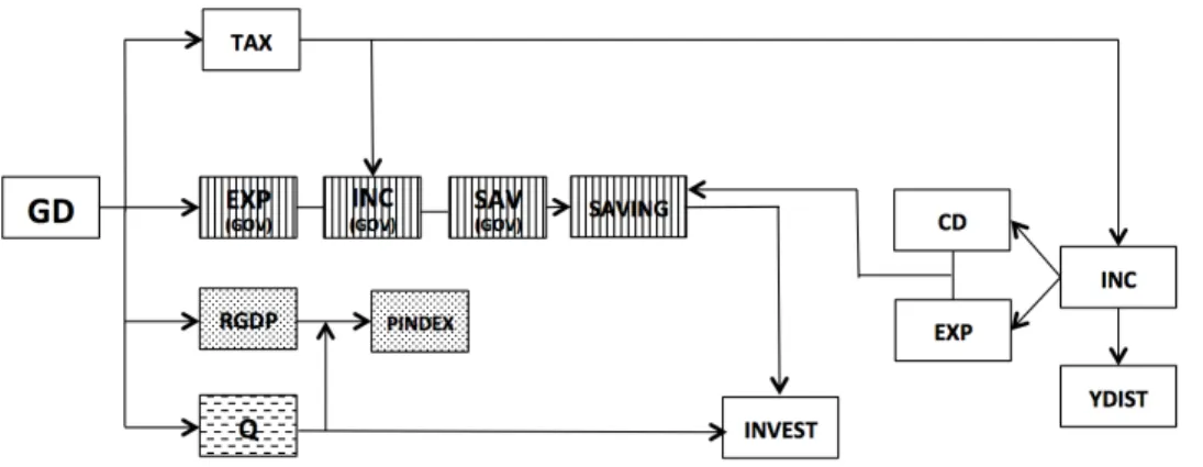
1.5. Immediate Transmission Channels by GD Increase in CGE Model ... 45
1.6. Immediate Transmission Channels by GD Increase in The FCGE Mode . 46 1.7. Comparing the Results from CGE and FCGE Simulations of GD Increase 47 1.8. Immediate Transmission Channels by GD Increase Through an Increase in Direct Tax in CGE Model ... 48
1.9. Immediate Transmission Channels by GD Increase Through an Increase in Direct Tax in CGE Model ... 49
1.10. Comparing the Results from the CGE and FCGE Simulations of GD Increase Through Tax ... 50
1.11. Comparing Results from FCGE Simulation of GD Increase Through Tax Increase and GB Issuance ... 53
1.12. Immediate Transmission Channels by GD Increase through GB Issuance in FCGE model ... 54
1.13. Comparing Results from CGE and FCGE Simulations of Capital Inflows ... 56
1.14. % Changes in Financial Income (left) and Income Distribution Under Capital Inflow Shock in the FCGE Model ... 59
2.1. Framework of Credit Channel Mechanism ... 73
2.2. Impact of A Tightening Monetary Policy with A Dynamic Credit Channel Mechanism ... 79
2.3. Flowchart Showing The Interrelationship of Variables in FCGE Model .. 92
2.4. Household Income Distributions: % Changes Between Non-credit and Credit Models ... 99
2.5. Income of Domestic Institutions: % Changes Between Static and Dynamic Models ... 102
2.6. Household Income Distributions: % Changes Between Static and Dynamic Models ... 102
2.7. % Changes in Real Sector Variables and Financial Returns under Risk- taking Behavior ... 103
2.8. % Changes in Income of Domestic Institutions under Bank’s Risk-taking Behavior ... 105
2.9. % Changes in Household Income Distributions under Bank’s Risk-taking
Behavior ... 107
2.10. Changes in Bank’s Income Composition During Outflow Compared to Baseline ... 114
2.11. % Changes in Incomes of Domestic Institutions during Outflow Compared to the Bank-led Inflow ... 116
2.12. % Changes in Household Income Distributions during Outflow Compared to Increased Bank-led Inflow ... 116
2.13. % Changes in Real Sector Variables During Outflow Compared to Bank- led Inflow ... 118
2.14. % Changes in Incomes of Domestic Institutions during Outflow ... 119
2.15. % Changes in Incomes of Domestic Institutions during Outflow ... 119
2.16. Changes in Financial Incomes of Domestic Institutions during Outflow 120 2.17. % Changes in Real Sector Variables under Bank’s Prudent Behavior . 120 2.18. % Changes in Income of Domestic Institutions under Bank’s Prudent Behavior ... 123
2.19. % Changes in Household Income Distributions under Bank’s Prudent Behavior ... 124
3.1. Basic Structure of ANP and AHP Models ... 152
3.2. AHP Model Structure of “Chances” ... 197
3.3. Supermatrix of ANP (left) and Entry in the Supermatrix (right) ... 161
3.4. The Whole Structure of ANP Model ... 166
3.5. The Whole Structure of ANP Model ... 167
3.6. ANP Model Structure of “Welfare” under Opportunities ... 169
3.7. ANP Model Structure of “Worsening Income Distribution” under Costs 172 3.8. Direct Data Input Method ... 193
3.9. Matrix Method ... 193
3.10. Questionnaire –Pairwise Comparison -- Method ... 194
3.11. Sensitivity Analysis for Each Variable under Benefits and Opportunities (1) ... 197
3.12. Sensitivity Analysis for Each Variable under Benefits and Opportunities (2) ... 198
3.13. Sensitivity Analysis for Each Variable under Costs and Risks ... 199
3.14. Sensitivity Analysis for Each Variable under Risks (1) ... 200
3.15. Sensitivity Analysis for Each Variable under Risks (2) ... 201
LIST OF TABLES
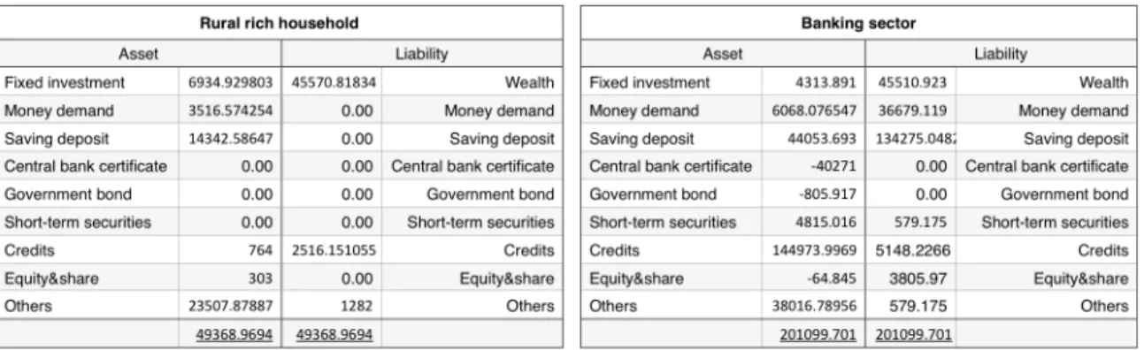
1.1. An Example of Balance Sheets Built According to FSAM ... 22
1.2. Variables in Each Block in CGE and FCGE Models ... 24
1.3. Summary of Three Different Key Channels in CGE and FCGE Models .. 43
1.4. Analysis Conducted in This Chapter ... 44
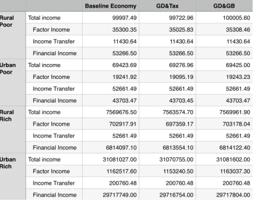
1.5. Comparing Household Incomes under Different Scenarios in FCGE Model ... 45
2.1. Wealth and Bank’s Loan in Non-credit and Credit Models ... 99
2.2. Changes in Bank’s Balance Sheet Between the Static and Dynamic Models ... 100
2.3. Absolute Changes in Bank’s and Firm’s Balance Sheets Showing Banks’ Risk-taking Behavior ... 106
2.4. Changes in Bank’s Balance Sheet Showing Bank’s Risk-taking Behavior during Bank-led Inflows ... 111
2.5. Changes in Bank’s Balance Sheet during Outflow Compared to Bank-led Inflow ... 112
2.6. Changes in Bank’s Balance Sheet During Outflow Compared to Baseline ... 114
2.7. Changes in Bank’s Income Composition during Outflow Compared to Baseline ... 122
3.1. Relative Intensity of Impact of CFLOW ... 155
3.2. The Normalized Results ... 155
3.3. Relative Impact of The Four Variables With Respect To Chances ... 155
3.4. Relative Importance of The Alternatives With Respect To Each Variable ... 156
3.5. Jointly Displaying The Relative Importance of All Elements ... 156
3.6. Joint Priorities of All Elements and Final Priorities of Alternatives ... 157
3.7. Supermatrices for “Chances” under Benefits from ANP model: Unweighted, Weighted, and Limit Matrices ... 164
3.8. Inputs from FCGE Simulations for BOCR ... 175
3.9. Overall Ranking for Each BOCR using AHP Model ... 176
3.10. Overall Ranking using ANP through Mutiplicative and Additive Synthesis ... 179
3.11. Overall Ranking using AHP through Mutiplicative and Additive Synthesis under Different Weights on BOCR ... 180
3.12. Overall Ranking using ANP through Mutiplicative and Additive Synthesis ... 181
3.13. Overall Ranking for Each BOCR using ANP through Mutiplicative and Additive Synthesis ... 186
3.14. Overall Ranking using ANP through Mutiplicative and Additive Synthesis under Different Weights on BOCR ... 187
CHAPTER 1
THE RISK OF NEGLECTING THE FINANCIAL SECTOR: THE CGE AND FCGE MODELS IN COMPARISON
1.1. Introduction
Whether we like it or not, a somewhat disturbing development has occurred in many countries around the world. While conceptually the role and development of the financial sector is meant to support the real sector of the economy, this has not been the case over the last several decades. The growth of the financial sector has far exceeded that of real sector. Several studies have sought to explain the reason behind such a trend where the key culprit is the combination of financial sector innovation with progress in financial technology and minimal regulation. This has happened in developed and developing countries alike, and emerging market economies are no exception. In fact, most financial crises in emerging market economies can be explained in one way or another by such a phenomenon. Financial globalization and deregulation further exacerbate the situation because there are no longer restrictions on the flows of capital. At any rate, the dynamics of economic growth and development in most emerging market economies has been significantly influenced by development in the financial sector.
It is well-known that the current global financial crisis has had negative repercussions on the advanced economies including the US economy. These repercussions, in turn, have also impacted many developing and emerging market economies worldwide. With globalization, where the financial sector has played an
increasingly important (if not the most important), the impact that started from the US financial market has flowed into the economies of other countries through their financial systems. These repercussions affect the real sector in various ways, such as high unemployment and a decrease in income, consumption and production as well as increased vulnerability of the financial sector. Any analysis omitting this sector, therefore, is bound to be misleading.
This chapter focuses on the comparison between the CGE and FCGE models. In particular, we impose some shocks on the two models and evaluate the transmission mechanism in each, upon which basis we then analyze the different results produced by the two models and argue that neglecting the role of financial sector in CGE can produce erroneous results. While the final results are important to compare, the transmission mechanism is even more important to understand because it sheds some light on the question of where and in which parts the government should intervene with its policy if a particular result is targeted. The CGE model itself is comprehensive enough to show such a transmission mechanism, and it allows us to implement a more accurate method when we wish to analyze the impact of a particular policy. Without this model, we are forced to analyze the policy impact by only examining a set of variables prior to the policy shock and then the same variables afterwards. This ‘before and after’ approach is flawed because it neglects the role of other things which occur simultaneously with the shock. A more accurate approach would be an approach that examines the situation ‘with and without’ policy shock. This can be done only if we have a model representing the economic system being analyzed. The CGE we are using in this chapter is an example of such models. In other words, the model is like a
laboratory for analyzing policy shock; however, as elaborated in this chapter, using the CGE model without incorporating the financial sector would undermine the accuracy of the results. Thus, it is in this context that we subsequently use a financial CGE (FCGE) model where a fairly detailed financial block is incorporated into the CGE model.
The FCGE model is based on an expanded SAM by merging the flow of funds into it. In this way, total investment and total saving in the standard SAM will be augmented by investment and saving in financial asset. Hence, the new total investment and new total saving basically consist of two components – the real sector and the financial sector – maintaining the equilibrium tradition of equivalent investment and savings in CGE. In the language of the financial balance sheet, total assets ought to equal total liabilities. There are two major components to total assets – fixed assets and other assets, which include financial assets. Investment in the standard CGE model, the data of which are derived from SAM, is nothing but the fixed asset or real sector investment. Therefore, the bulk of other assets consists of financial assets such as securities, equities, and loans. On the liability side, the saving from the CGE model, derived from SAM, is equivalent to the wealth or net worth. For example, in the case of banks, these items typically consist of deposits made by the public and in some cases also loans from other banks (inter-bank loans) or other institutions. In recent years, many banks in emerging market economies have also raised financing from external sources. Given the ultra easy money policy in the advanced economies, especially after the global financial crisis, the incentive for many banks in emerging market economies to acquire external funding has increased significantly because the
cost of such funding is very low. For example, the short-term annual interest rate in the United States fell dramatically from in 5.30 in 2007 to 0.43 percent in 2012 (see Figure 1.1). Similarly, the short-term interest rate adopted by European Central Bank fell from 4.28 in 2007 to 0.57 percent in 2012. This ultra easy money policy combined with Quantitative Easing (QE) has sparked massive capital outflows from advanced economies, most of which has gone to emerging market economies. Many banks in the latter have taken advantage of such an environment, raising the share of non-core liabilities (liabilities outside of deposits). At any rate, increased capital inflows have become a major phenomenon in most emerging market economies.
Figure 1.1. Short-term Interest Rates: Three-month Interbank Rates: Annual Average Percent (Square= Euro Area, Dot = USA)
Following of the collapse of Lehman Brothers in the fall of 2008, the US economy fell into crisis. Subsequently, the economy of the Euro Zone area also encountered trouble. Both resulted in a global financial crisis, which also affected many emerging market economies. As a response, policymakers in emerging market economies have attempted to counter the downward pressure by implementing a series of stimulus policies. While there are several types of stimulus policies, almost all countries have used a fiscal stimulus by raising government spending. Given that most emerging market economies suffer from the perennial problem of worsening income inequality, it is expected that most of the physical stimulus are directed towards sectors that they believe will help raise the income of the poor while at the same time having a sufficiently large multiplier in the economy. Agriculture, construction (building), and trade fall in this category.
Given what is described above, in this chapter we impose a shock in terms of increased capital inflows and increased government spending in these three sectors. In raising government spending, we compare three cases: in the first case, no particular efforts are made to determine the sources of financing for the increased spending; the second case is based on raising direct taxes to finance the increased spending; and the last case finances the spending through government bond issuance.
We examined results from the CGE and FCGE models that demonstrate how the transmission mechanisms of the CGE model can be misleading and how the FCGE model differs from the real sector model. In particular, the equations defining the income of domestic institutions were modified such that the overall income includes
not only the factor income and income transfers from other institutions but also the income from financial investment (financial income). The resulting total income that includes earnings from financial returns is thus different from the income specified in CGE model.
1.2. Literature Review
One of the desirable features of economy-wide models is their ability to explicitly capture the link between micro and macro variables such that one can evaluate how the behavior of agents can influence and be influenced by the macro aggregates. When banks are taking more risks by investing in securities or derivatives instead of lending to the business sector, they will not stimulate real sector growth (GDP), which in turn will make banks more vulnerable. On the other hand, when the economic growth slows down because of, say, falling exports due to the global crisis, firms may decide to postpone their investment, and consumers may cut their spending, causing the economy to fall into recession. The nature and intensity of the abovementioned causal effects depend on the model specifications and the exact size of the parameters, all of which should reflect the behavior of different agents. Arguably, some equations in the model are non-linear. This is the essence of computable general equilibrium (CGE) models.
The basic theoretical underpinning of CGE frameworks is Walras’ model of a competitive economy. The formal statement of a Walrasian economy can be found in the classic general equilibrium theory of Arrow and Hahn (1971) and Debreu (1959).
Scarf (1973) made the determination of the equilibrium of a Walrasian system possible. Calibration of the model parameters is based on real data to provide the empirical content to the purely axiomatic general equilibrium theory of Arrow-Hahn-Debreu.
The lineage of CGE models can be traced to the early work of Johansen (1960), who developed a linear model to deal primarily with distributional issues in Norway. In the model, quantities and prices are simultaneously determined with sectoral reallocation of labor and capital. This early category of CGE was of the neo-classical type, where producers are assumed to be profit maximizers in perfectly competitive markets, consumers are utility maximizers, and production factors are paid according to their marginal productivity. The solution of such a system provides a set of prices that clears all markets in one single instance, implying the presence of resource constraints (e.g., budget constraints) and full employment. The model is saving-driven, and no investment function is specified.
In the 1970s, the popularity of multisectoral analysis and macro models took off; most were used for policy analysis in developing countries. In general, the objective of using CGE is to analyze the quantitative effects of exogenous changes on the optimal allocation of resources, efficiency and welfare. In retrospect, this seems rather peculiar since most assumptions employed in the neo-classical CGE models do not hold in developing countries. Prices are not always formed by market clearing, and full employment condition is almost non-existent. At the time, the primary goal of the model was not to describe actual economies; instead, it was meant for constructing a ‘mental organizing framework’ that could be used to analyze a set of policy issues.
As efforts to reflect the actual economy grew, model conditions became less strict. Although the models are still generally based on optimizing representative agents and markets are cleared by endogenous prices, in some sectors the quantity clearing markets
are not required. Certain production sectors are not modeled (Taylor, 1990). This is a departure from the standard neo-classical Walrasian CGE model.
Further development of CGE models puts the focus on the short-run income distribution, sectoral growth and trade balance effects, and less on resource allocation effects of exogenous shocks (Thissen, 1998). Behavior of economic agents is not necessarily derived from optimizing behavior. There is clearly a trade-off between keeping the internal rigor and the empirical relevance of the model, and the latter prevails. At the time, the use of CGE models for trade policy analysis was quite popular because most of the effects surrounding trade policy, such as those captured in the Stolper-Samuelson Theorem, are general equilibrium in nature. A good early survey of CGE models can be found in de Melo (1988) and Francois and Shiells (1994).
Meanwhile, new developments also took place on the data front. In recognition of the fact that household income distribution had become politically and economically more important than the traditional functional income distribution (i.e., between wage earners and capital owners, as traditionally used in the input-output framework), efforts were made to construct a comprehensive yet consistent data system that depicts the link between production and other blocks of the economy with the household income distribution. Such a data system, known as the Social
Accounting Matrix (SAM), also captures other sources of income outside factor income, such as transfers between different institutions. Clearly, this reflects the reality better and hence is more relevant than the input-output data system.
The SAM data system has other advantages as well. In the international trade context, one may want to analyze the average tax rate on imported goods and the proportion of imports of certain goods to the total supply. Often, it is also necessary to capture the impact of increased imports, say, due to tariff reduction on household incomes. Information of this nature cannot be investigated through input-output models. One may also wish to know the shares of non-factor incomes (transfers) received by different institutions (firms, government, banks, households) from abroad. Such information is absent in input-output but available in SAM. More generally, the analysis of capital flows can be made more accurately by using information from SAM. Structuralist CGE modelers took advantage of this development on the data front. Using SAM data, the structuralist models are demand-driven, unlike the saving-driven neo-classical model. A seminal work by Adelman and Robinson (1978) is a notable example. They are also among the first to attempt to integrate functional and household income accounts in the tradition of a SAM into a CGE model. A bibliographic survey of CGE models that have been applied to 26 developing countries, including the structuralist models, can be found in Decaluwe and Martens (1988). The countries covered by this study vary in their standard of living, policy orientations, degree of openness, and stage of industrialization. Another systematized account of CGE models can be found in the surveys done by Gunning and Keyzer (1995), and Ginsburgh and Keyzer (1997).
Among several components, closure in the models plays a critical role as it allows us to distinguish among different types of CGE models. Different types of closure give different results even when the structures of the two models are the same. In the neo-classical models, the closure specifies that aggregate investment is determined by aggregate saving, which is in turn determined endogenously through a fixed savings rate out of the after-tax income and government deficit. In the Johansen model, the closure specifies that aggregate investment is fixed exogenously and the savings rate is assumed to adjust in order to generate the required savings. Johansen (1974) argues that fiscal and monetary policies need to ensure that the generated savings will equal investment.
In a Keynesian framework, wage is usually set as the numeraire (also common in structuralist model, see Taylor, 1983, 1990). Investment is fixed, but labor supply is assumed to be endogenous. The adjustment in real wages is the macro equilibrating mechanism, while aggregate price is the equilibrating variable. If investment increases, savings must increase through rising income, which requires increased employment and output by way of falling real wages. To reach an equilibrium point, the latter requires an increase in the aggregate price. It is through this mechanism that the Keynesian multiplier is derived: an increase in investment yields a new equilibrium level of output, which equals to the multiplier [1/(1-mpc)] times the investment increase. The model yields the same results if price level is chosen as the numeraire (wages become the macro equilibrating variable). The equilibrating mechanism in this case is as follows: real wages will adjust to create the employment necessary to generate income, the level of which will ensure that savings are equal to
investment.
Another type of Keynesian closure is where the price level is set as the numeraire and real wages are fixed. Labor supply is set free, so employment is not fixed. In contrast to the earlier Keynes specification, firms here are not in the demand curves for labor. A labor distortion parameter is hence introduced. This parameter measures the degree to which wages deviate from the marginal product of labor, and it will adjust until firms are induced to hire labor at fixed wages necessary to generate the income that will produce savings equals to investment.
In interpreting the distortion parameter, Barro and Grossman (1976) argued that since product and labor markets are out of equilibrium, firms are forced off their labor demand curves. The distortion parameter measures how far off they are. Another interpretation by Malinvaud (1977) emphasizes that firms are demand-constrained and rationed in the product market, and the distortion parameter measures the degree of this rationing. Either way, the equilibrating mechanism will be the same, i.e., employment is demand-determined, Keynesian multiplier is at work, and real wages remain constant.
While comprehensive and based on a robust economic theory, there is one important component missing from CGE models, i.e., the financial sector. Yet, irrespective of the economic system adopted, the role of the financial sector in most countries around the world is so great, especially in the post-liberalization period, that all aspects of the economy are directly and indirectly affected by the dynamics of this sector. When a fairly detailed financial module is incorporated into CGE, the simulation results of any shock are likely to be different than those generated by CGE models without a
financial module. The distinction between CGE with and without a financial module can be better explained by their respective simulation results when a particular shock is imposed in both models. In this chapter, I will do precisely that by analyzing the case of an emerging market economy – Indonesia.
Thissen (1999) provided an overview of financial CGE (hereafter ‘FCGE’) models. He shows the superiority of FCGE over standard CGE models in analyzing the stabilization and structural adjustment (SSA) programs advocated by the World Bank and the IMF in the 1980s. He argues that CGE models are inadequate to analyze the interactions between the real sector and the financial sector, resulting in inaccurate conclusions. Robinson (1991) surveyed FCGE models by emphasizing the role of loanable funds in micro and macro CGE models.
Despite their superiority, FCGE models also have some limitations. Thissen (1999) identified the following: (1) the difficulty to acquire financial data, especially different types of financial assets held by different agents; (2) the interactions within the financial sector as well as between the financial and real sector are often simplified; and (3) the parameters may need to be guesstimated, adopted from other studies, or assumed, due to the lack of readily available data.
Goodhart, Sunirand and Tsomocos (2004, 2005) emphasize the modeling of international financial flows and its effects, and disaggregate net investments by type of investor, banks, firms and the rest of the world. They also take into account the possibility of default to depict a financial fragility condition. Maldonado, Tourinho and Valli (2007) provide another example of an FCGE model where foreign capital flows are treated endogenously. Using the case of Brazil, they link capital flows with
the expected rate of loss of foreign reserves. Simulating the model for the case of Brazil joining a free trade agreement (FTA) as part of the trade policy, they conclude that the impact is significantly larger than without financial flows precisely because the financial flows amplify the impact of the policy.
Azis (2000a, 2000b) used an FCGE model to analyze the impact of the Asian financial crisis in 1997 on a set of social variables. By detailing the intricate mechanisms within the product and factor markets, and linking them with the financial market, he highlighted the role of real wages where urban households suffered more than rural households. In his subsequent and related work (Azis, 2001 and 2002), he used this structure to explain the phenomenon of reverse migration (from urban to rural). One of the key findings of his work is that the financial sector can play a significant role in affecting income distribution between different households. By adding a poverty module, he was also able to link the financial crisis with the trend of poverty where the poverty line and the income of poor households (i.e., the two determining variables in poverty measure) are endogenous.
Morley, Pineiro and Robinson (2011) developed a dynamic real-financial CGE model for Honduras. The key feature of their model is the incorporation of working capital as an additional factor of production, complementary to physical capital. This is considered to be important for short-run macro and trade policy analysis. Based on SAM, the model is recursive dynamic with short-run unemployment, where minimum wage is fixed and informal sector is treated explicitly. With the treatment of working capital, they examine the impact of monetary shocks that affect the supply of credit on the balance of payments, employment, and real income.
The use of flow and stock data is another important issue in FCGE modeling. Most data are usually denominated in flows, but models that allow for complete portfolio restructuring are preferred, in which both the stock and flow data are used simultaneously. An example of such models, also used in this chapter, is the portfolio model of Tobin (1967). Thorbecke (1991) is among those who used Tobin’s portfolio model to analyze various SSA policy scenarios in the case of Indonesia.
In terms of the time dimension, CGE and FCGE models are generally suitable for analyzing medium-run repercussions of policy changes. The extent of model simulations should be long enough to allow for prices to adjust but short enough to assume that the model parameters are stable. Some also tried to construct dynamic CGE models to address various long-term issues ranging from long-term growth to environmental problems such as climate change. The dynamic models simulate the economic equilibrium for several successive moments in time, which are linked recursively though the trajectories of the state variables (see Rutherford and Tarr, 2005; Azis, 2009).
The model used by Morley, Pineiro and Robinson (2011) is another example of a dynamic CGE model with the financial sector. It is recursive dynamic, solved in two stages. First, the model determines a within-period equilibrium, given parameters and exogenous variables, then some parameters and exogenous variables are allowed to change over time. The model contains transition equations that determine how the exogenous variables and parameters relate to past solution values for particular endogenous variables. In some cases, these variables are assumed to grow according to trends. These transition equations provide values for all exogenous variables and
parameters for the next period for the static CGE model, which is then updated and solved for a new within-period equilibrium. In essence, they used the model to solve forward in a dynamically recursive fashion, with each static solution depending only on current and past values of variables and parameters. What is important to note about this feature is that the behavior of agents is based on historical information and adaptive expectations. It does not need to assume that agents have knowledge of the future. As in most dynamic models, the variables and parameters used as linkages between periods are the aggregate capital stock, exogenously determined population, domestic labor force, supply of working capital, factor productivity, export and import prices, export demand, tariff rates, and transfers to and from the rest of the world.
1.3. Methodology
1.3.1. The Dataset of The CGE Model: Social Accounting Matrix (SAM)
The Computable General Equilibrium model is descendant from the input-output (I-O) model pioneered by Wassily Leontief. The CGE model is based on the SAM dataset that includes the I-O model as a production sector. SAM is an integrated dataset consisting of national accounts, balance of payments, government budget, input-output table, and socio-economic surveys. SAM consists of multiple production sectors, multiple factors, and multiple institutions in matrix form. Each account interacts with the others in a circular fashion, providing a comprehensively detailed and quantified description of an economy. The SAM provides snapshots of the economy at a single point in time, and each cell of the matrix represents the value
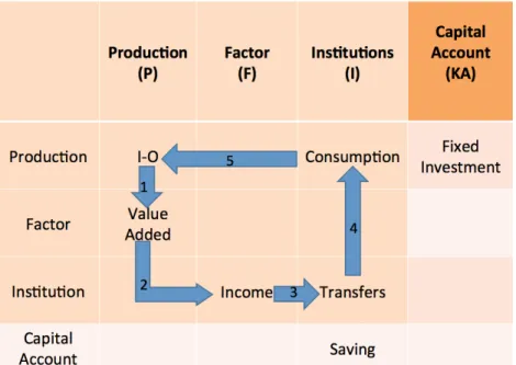
of each transaction. There are five steps that form each cycle (see Figure 1.2): (1) Production activities captured in the I-O table generate value added – labor and capital – as factor income from the production activities; (2) factor income is distributed to the institutional sectors, which decide income distribution among households; (3) after paying taxes and transferring the income within different institutions; (4) the income is used by each institution to consume commoditiesfrom the production sectors while excess income is saved; and (5) this consumption pattern takes into account production activities affecting the level of output, export, and import. The new level of production activities generates a new level of value added and so forth. This circular flow represents the interdependency within/among production activities, production factors, income distribution, consumption, and transfer activities.
The interactions are captured in multipliers (𝑀!"#) calculated by the following:1
y x
y 𝑫𝒚𝒚 𝑫𝒚𝒙
y=f(x,y), where y is a set of endogenous variables and x is a set of exogenous variables.
dy = [𝐼−𝐷!∗𝐹 𝑥,𝑦 ]!!𝐷
!* 𝐹 𝑥,𝑦 dx = [𝐼−𝐷!!]!!𝐷!" dx
dy = 𝑀!"#∆𝑥
Any change in the exogenous variable (∆𝑥) will alter the endogenous variable y by
𝑀!"#.
As a data system, however, SAM has some limitations in evaluating the impacts of the changes in one part of the economy on the rest because SAM as a data system assumes excess capacity, perfect elastic supply, linearity and no substitution effect. SAM also does not take into account behavioral features, and does not contain prices that play an important role as incentives in an economy. In other words, in SAM, there is no automatic partition of the transactions into the price and quantity. When there is a change, either from exogenous shock or endogenous change in demand and supply, the structure decides the magnitude of the change represented by the change in quantities but not in the change of prices. Although SAM is useful and comprehensive as a data system and modeling tool, a further extension is needed from the modeling point of view. One such extension is to endogenize the prices, to capture some optimizing behavior of different agents, and to allow the presence of excess capacity, different technology and substitution. This is where the computable general
1 From Robinson, S., and Roland-Holst D.W., (1998)
2 The values of excess market demands equals the values of excess market supplies
equilibrium (CGE) model is distinguished from the dataset as a model.
1.3.2. The CGE model
The CGE model is based on the SAM dataset with prices assigned an endogenous role. When economic agents meet in the market, endogenous prices arise in the system that satisfy Walras’ law.2 CGE or Jacobian multipliers can show the difference between SAM as a data system and the CGE model.
CGE or Jacobian multipliers:
y Z x
Y 𝑫𝒚𝒚 𝑫𝒚𝒛 𝑫𝒚𝒙
Z 𝑫𝒛𝒚 𝑫𝒛𝒛 𝑫𝒛𝒙
With the endogenous prices, the following system applies to the CGE framework. y=J(x,y,z), where y (quantity) and z (price) are both endogenous, and x is a vector of exogenous variables. A Jacobian multiplier can be derived:3
dy = [𝐼−𝐷!!+𝐷!"(𝐼−𝐷!!)!!𝐷
!"]!! 𝐷!"+𝐷!" 𝐼−𝐷!! !!𝐷!" 𝑑𝑥∗𝐽(𝑥,𝑦)]!!
=𝑀!!"#∆𝑥
dz = 𝑀!!"#∆𝑥
The Jacobian multiplier (MzCGE and MyCGE) captures the equilibrium
dependence of the endogenous variables on one another as well as on exogenous
2 The values of excess market demands equals the values of excess market supplies
3 Sherman Robinson, David W. Roland-Holst, Macroeconomic structure and computable
general equilibrium models, Journal of Policy Modeling, Volume 10, Issue 3, Autumn 1988, pp. 353-375.
shock. If the three components (Dyz, Dzz and Dzy ) in CGE are set to zero, then the
above Jacobian multiplier becomes the SAM multiplier (Msam). The SAM multiplier does not include prices, whereas the Jacobian multiplier takes prices in the system into account. The off-diagonal elements (Dyz, Dzy) denote linkages with prices. Dzz reflects
the price interaction in the system, e.g., a policy lowering prices of some upstream industries has a favorable effect on the prices of some downstream industries. Hence, while the elements in the SAM multiplier matrix are positive numbers, the elements in the Jacobian have negative values reflecting the changes in prices. For example, demand increase for food processing industry will have a favorable impact on some agriculture sectors, which generates a positive multiplier; however, the increasing demand in agriculture products may have a negative impact on food processing because it raises prices of the forward industry's input market, which gives the multipliers negative values. Therefore, while the SAM multiplier results from an assumption of the excess demand, the Jacobian multiplier is adjusted according to price changes that extinguish the excess demand.
The CGE model is a deterministic model, not stochastic like most econometric models. It calibrates parameters and consists of a set of simultaneous equations. Thus, the CGE model has no pre-determined objective functions, while econometric models allow the error term (residual). Instead, the CGE model contains a set of equations that are numerically solvable and facilitate the ability of economic agents to find the best solutions given various macro and accounting constraints: the budget constraints of households and governments, the balance between trade balances, and the balance of payments. The CGE model is structured by equation blocks containing
characteristics of the economy: (1) production block; (2) price block; (3) income block; (4) expenditure block; (5) market clearing block; (6) GDP & utility block; (7) distortion block; (8) subsidy block; and (9) transfer block. Each block contains a set of corresponding equations. These blocks will be explained in detail in the FCGE model section.
The CGE model consists only of real sector variables mentioned above as the SAM dataset deals with real sector savings and investment in one combined account. Treating each real sector saving and investment as one capital account misses one of the most dynamic sectors in the economy – namely, the financial sector. One might argue that in SAM, the relationship between real sector and financial sector performance might be somehow explained by using one capital account that contains gross savings and investment information of institutions. Given that real sector investment depends not only on economic agents’ own savings but also on bank loans and other financial assets, in reality, savings are not only spent on physical assets but also on financial assets. In particular, the source of funds for investments can also come from other sources, such as loans, deposits, and savings. Such transactions became very critical since the Financial Sector Liberalization (FSL) in the 1980s. In almost all developing countries, financial assets play an important role as an alternative source of financing for banks. As financial institutions and instruments have been developed, the asset markets have become a crucial means for the investments and savings of economic agents. Therefore, the transactions cannot be bundled into one account and cannot be analyzed in the same way that SAM treats the capital accounts. Without the financial sector in the system, the analysis may be
biased, especially for social issues such as poverty analysis. While every investment is assumed to generate employment in models without the financial sector, investment in financial assets may in fact not be generating employment. Also, a financial boom may inflate asset prices and hence affect other social indicators – the poverty line and income – through inflation, while the effects maybe underestimated in the CGE model without this explicit channel. In addition, the absence of the financial sector excludes the fact that investors in financial assets are not poor households and hence income distribution may be worsened when financial assets are incorporated into their income. Given the critical role of the financial sector in modeling and in reality, the sector should be specified and allowed in the model to acquire accurate economy-wide impacts from any shocks or policies. When it comes to policy analysis related to the financial sector, the CGE model without any financial accounts is not adequate.
1.3.3. The Dataset of The FCGE Model: Financial Social Accounting Matrix (FSAM)
As mentioned earlier, although the CGE model is useful to analyze economic impacts on the real sector, neglecting the behavior and specifications of the financial asset market can mislead the analysis of any economic impact.
The Financial Computable General Equilibrium model introduces asset markets and loanable funds markets by disaggregating the capital account in SAM and incorporating the flow of funds (FOF) table into the dataset, which now becomes the Financial Social Accounting Matrix (FSAM). The FOF contains most flows of investments and savings occurring from simultaneous decisions of economic agents,
which allows us to track where the different assets of various institutions are being spent and used. Based on the FOF, the savings and investments in the capital account of SAM are disintegrated into investments for the real sector (investment), investments for the financial sector (assets), savings from the real sector (savings), and savings from the financial sector (liability), (see Figure 1.3). In SAM with the FOF, thus, it can be elaborated that saving consists of saving and wealth, while total investment consists of physical investment and financial investment.
Figure 1.3. Structure of FSAM Matrix and Its Circular System.
By incorporating FOF, the FSAM can elaborate information on the assets and liabilities of the financial sector as well as savings and investments of the real sector. The model based on the FSAM finally is able to specify the loanable funds markets with a variety of different assets, such as currency, demand deposits, saving deposits, time deposits, central bank certificates, government debt (bonds), other long-term securities, short-term securities, working capital credit, investment credit, consumption credit, non-bank credit, trade credit, equity and shares, and insurance pension fund reserves. This information appears to be the balance of payment for each institution as shown in Table 1. FSAM can provide a consistent and coherent statistical framework for both the real and financial sides of the economy. Hence, whereas most macro-econometric models imperfectly specify flows of income among agents, the FCGE gives a comprehensive and detailed quantified description of the macro-economic and financial interrelations by linking the real sector, the social sector, and the financial sector.
1.3.4. The FCGE model
The FCGE model takes into account endogenous prices in the system like the CGE model. In addition to the prices in the real sector, the FCGE model includes financial asset prices, allowing us to analyze the impact associated with asset prices, such as price bubbles, which precluded many past crises.
Figure 1.3. Interrelationship among the blocks in the FCGE Model
Table 1.2. Variables in Each Block in CGE and FCGE Models
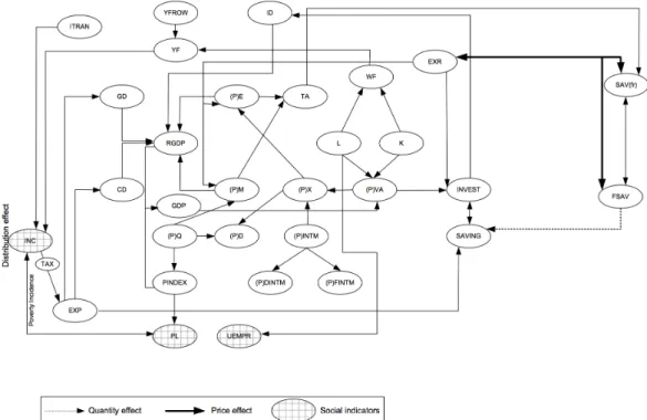
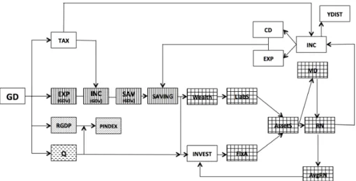
With detailed information on the financial activities of each institution, the FCGE model is structured both by CGE blocks containing real sector variables (1 to 9) and by FCGE blocks containing financial sector variables (10 and 11): (1) production block; (2) price block; (3) income block; (4) expenditure block; (5) market clearing block; (6) GDP and utility block; (7) distortion block; (8) subsidy block; (9) transfer block; (10) financial block; and (11) currency and demand deposit block as shown in Table 1.2. Each block includes a set of equations and its corresponding variables. The production block contains export (E), import (M), factor demand (FACDEM), supply (Q), value added (VA), intermediate inputs (INTM), and taxes. The price block consists of each price of the production variables and price index (PINDEX). The income block has variables and equations for factor income (YF) and total income (INC) after transfers. The expenditure blocks are for the relationships among consumption (CD, GD), saving (SAV), foreign saving (FSAV), investment (INVEST), expenditures (EXP), investment demand (ID), and exchange rate (EXR). The unemployment variable (UEMP) is in the market-clearing block. GDP and utility blocks contain variables and equations regarding yield GDP and RGDP. The distortion block is for tariffs (TARIFF), indirect taxes (IDTAX), and imperfect competition (IMPERFECT). The subsidy block contains subsidies to export, import, and households given by government. Transfer variables and equations are included in the transfer block. Government transfers (GTRAN) is included in income transfers (ITRAN). Financial blocks show the relations through the equations for financial assets (Asset, AssetSLag, and AssetS), liabilities (Liab, LiabSlag, and LiabS) and corresponding financial returns (RN and AvgRN). The money demand (MD) of
institutions, consisting of currency and demand deposit, is included in the currency and demand deposit block. All blocks dynamically interact with each other in the FCGE model. Especially, (10) financial block and (11) currency and demand block only exist in the FCGE model, taking into account the transactions from FOF information. The connections between real sector blocks (1 to 9) and financial sector blocks (10 to 11) represent the interaction between real and financial sectors in an economy. In the income block of the FCGE model, financial income – defined as return (RN) multiplied by financial asset (Assets) – is added to the total income (INC). As part of the income (INC) of each institution, any changes in the financial sector will alter financial income, resulting in changes in total income. Also, part of the investment originally intended for financial sector (Asset) can be used for real sector investment (INVEST) – secondary investment channel. The increase of financial wealth therefore can lead to real sector investment increases in the real sector. In addition, money demand (MD) of the economic agents as part of financial assets plays an important role in the economy. Affected by income and interest rates, the money demand also subsequently affects the income of the institutions through changing financial return (RN) and asset composition, affecting consumption (CD) and production activities sequentially, i.e., central bank’s income. Furthermore, the FCGE model incorporates behavioral aspects associated with the investment of each institution in financial assets. Economic agents’ decisions as to how much to invest in which financial assets affects their wealth and thus the entire economy. The decision criteria whereby economic agents allocate their wealth (money) to various financial assets, in particular, are essential to the income of households, as well as profits of
firms and the government. Furthermore, the criteria can often be influenced by shocks or policies. Although the FCGE model is a bridge between the real sector and the financial sector, the model itself does not provide a complete explanation of the actual behavior of economic agents in allocating their wealth in financial assets. The FCGE used in this thesis takes into account Tobin’s theory to incorporate the behaviors of institutions into financial asset allocation. In this model, only the allocation theory for rural households is applied.
According to Tobin, the decisions of economic agents or investors depend not only on the relative returns on financial assets but also on risk factors in investing the financial assets. In other words, the risk factors involved in possessing the asset influence investors' decisions. Tobin’s theory captures both criteria as follows:
𝑔ℎ1!!
1−𝑔ℎ1!! = 𝑝ℎ𝑖ℎ1!!∗(
1+𝑅𝑁𝐷𝑃
1+𝑅𝑁𝑁𝐷𝑃)!"#!!!!
𝑔ℎ1!! is an allocation variable as to how much rural households allocate their money to demand deposit. 𝑝ℎ𝑖ℎ1!! and 𝑒𝑠𝑝ℎ1!! are risk parameters. RNDP is the return on demand deposit, and RNNDP is the return on other assets excluding demand deposit. 𝑒𝑠𝑝ℎ1!! is a risk that is embeded in the return on the asset, in this case demand deposit; whereas 𝑝ℎ𝑖ℎ1!! is a external risk that exists other than the financial asset, i.e., regulations, and financial crises from other countries. If there is a case of no risk in the financial asset, then the risk parameter, esph1rh, is set to zero,
leaving the right-hand side one. In reality, however, other external inflences exist to keep the investors from putting money in demand deposit accounts. 𝑝ℎ𝑖ℎ1!!
The model with detailed information about the financial assets and liabilities of institutions, thus, is empirically more reliable. Furthermore, given the interplay between the real sector and the financial sector in reality, any policy and/or impact analysis that does not consider the impact of the financial sector will be misleading. Therefore, especially for policy analysis with financial variables, a financial CGE model where the financial sector is specified in greater detail is preferable to a standard CGE model.
1.3.5. Comparing The CGE and FCGE models4
In the previous section, the presence of a financial block and demand deposit block distinguishes the FCGE model from the CGE model as shown in Table 1.2. This section articulates and compares the channels and their effects –Feature 1.1, Feature 1.2, and Feature 1.3 – these effects distinguish the FCGE model from the CGE model.
Figure 1.3. The Interrelationship Among the Variables in The CGE Model
Figure 1.4. The Interrelationship Among The Variables in The FCGE Model5
Feature 1.1. Quantity effect: total investment = total saving
CGE: 𝐼𝑁𝑉𝐸𝑆𝑇!" = 𝑆𝐴𝑉𝐼𝑁𝐺!"
Total physical investment = Total saving from real sector FCGE: 𝑇𝐼𝑁𝑉𝐸𝑆𝑇 = !"(𝐴𝑠𝑠𝑒𝑡𝑆!",!")+𝐼𝑁𝑉𝐸𝑆𝑇!"
Total investment = Total financial sector investment + Total real sector investment TSAVING= !"(𝐿𝑖𝑎𝑏𝑆!",!")+𝑆𝐴𝑉𝐼𝑁𝐺!"
Total saving = Total financial liability + Total real sector saving
𝑇𝐼𝑁𝑉𝐸𝑆𝑇 = 𝑇𝑆𝐴𝑉𝐼𝑁𝐺
Feature 1.1.1. Investment
CGE:Physical investment alone
• 𝐼𝑁𝑉𝐸𝑆𝑇= ! !"𝐼𝑁𝑉𝐸𝑆!,!" (Eq. 1)
Total Physical Investment by all institutions
• 𝐼𝑁𝑉𝐸𝑆!,!"# =𝑙𝑎𝑚𝑏𝑑𝑎0!,!"#$∗𝑉𝐴!"#$%"! !!∗ 𝐴𝑣𝑔𝑅𝑁 !"#$%"!!∗𝐸𝑋𝑅!"#$%"!! (Eq. 2) Real sector investment by firms is affected by value added, interest rate, and exchange rate. avgRN is an average asset of the returns on 17 financial assets. VAi is the value added in sector i (output accelerator). EXR is the exchange rate, and AvgRN is the average return rate. 𝜆!!,𝜆!!,𝜆!!,𝜆!! are constant (positive, positive, negative and negative, respectively).
FCGE:Physical + financial investment
• 𝐹𝑖𝑥𝐴!" = !𝐼𝑁𝑉𝐸𝑆!,!" (Eq. 3) Total flow of physical investment by the institutions, which is the same as Eq. 1
• 𝐹𝑖𝑥𝐴𝑆!" =𝐹𝑖𝑥𝐴𝑆𝐿𝑎𝑔!"+𝐹𝑖𝑥𝐴!" (Eq. 4)
Total physical investment at the end of period consists of the real sector investment at the beginning of period and the change between two periods.
• 𝑇𝐼𝑁𝑉𝐸𝑆𝑇= !"( !"(𝐴𝑠𝑠𝑒𝑡𝑆!",!")+𝐹𝑖𝑥𝐴𝑆!") (Eq. 5)
Total investment that occurred both in the real and financial sector in an economy
• 𝐼𝑁𝑉𝐸𝑆!,!"#$=𝑙𝑎𝑚𝑏𝑑𝑎0!,!"#$∗𝑉𝐴!!"!"#$!!∗ 𝑎𝑣𝑔𝑅𝑁 !"#$%"!!∗𝐸𝑋𝑅!"#$%"!!
(Eq. 6)
In the CGE model, ‘investment’ means investment in the real sector or physical investment as shown in Eq. 1; however, in reality, economic agents invest not only in physical products such as land, building, and machines but also in financial instruments. In the FCGE model, investment (Eq. 5) includes financial investments, such as investment in stocks as well as physical investment. The total investment box in Figure 2 includes both. Both physical and financial assets consist of the stock at the beginning of the period and changes within the period, yielding a total stock value at the end of the period. Furthermore, the investment of firms (Eqs. 2 and 6) in both models depends on the value added (VA), average interest rate (AvgRN), and exchange rate (EXR). The average interest rate in the CGE model is an equilibrating factor to adjust the level of real sector investment of financial institutions, whereas the AvgRN in the FCGE model is an average weighted return on all financial assets (Eq. 25). The domestic investment depends on the economic cycle – value added – positively, interest rate negatively, and exchange rate negatively. If EXR collapses, as it often does during crises, institutions with high leverage on short-term and un-hedged foreign debt experience magnified debt burdens. Also, since the returns are endogenously weighted in the FCGE model, any changes either from real or financial sectors in the economy can alter the rates. The interaction through returns will be explained in detail in Feature 1.2.
Feature 1.1.2. Savings
CGE: Saving solely from real sector activities
• 𝑆𝐴𝑉!"#=𝐼𝑁𝐶!"#−𝐸𝑋𝑃!"# (Eq. 7) Saving by domestic institutions is their income after taking into account expenditures