A Singularity-Robust LQR Controller for Parallel Robots
Ricard Bordalba, Josep M. Porta, and Lluís Ros
Abstract— Parallel robots exhibit the so-called forward singu-larities, which complicate substantially the planning and control of their motions. Often, such complications are circumvented by restricting the motions to singularity-free regions of the workspace. However, this comes at the expense of reducing the motion range of the robot substantially. It is for this reason that, recently, efforts are underway to control singularity-crossing trajectories. This paper proposes a reliable controller to stabilize such kind of trajectories. The controller is based on the classical theory of linear quadratic regulators, which we adapt appropriately to the case of parallel robots. As opposed to traditional computed-torque methods, the obtained controller does not rely on expensive inverse dynamics computations. Instead, it uses an optimal control law that is easy to evaluate, and does not generate instabilities at forward singularities. The performance of the controller is exemplified on a five-bar parallel robot accomplishing two tasks that require the traversal of singularities.
I. Introduction
Parallel robots may be advantageous because of their stiffness, precision, and the efficiency of their movements [1]. These assets come at a high cost however: their workspace tends to be limited, and the planning and control of their motions are rather involved. Their closed kinematic chains and passive joints give rise to forward singularities [2], [3], in which the system becomes underactuated [4]. In such configurations, thus, the system will be unable to follow arbitrary accelerations. Actually, for some accelerations, the inverse dynamic problem will yield extremely large motor torques.
It is important to note, however, that singularity-crossing motions can safely be executed if the kinodynamic con-straints of the robot are respected [4], [5], [6], [7]. This is a key finding, because the motion capabilities of the robot can be greatly enlarged if such motions are allowed. A recent planner, in fact, is able to generate singularity-crossing motions [8], [9]. This planner relies only on for-ward dynamics, and thus obtains trajectories that fulfill all kinodynamic constraints, even at the forward singularities. These trajectories are “open loop” though, and thus they need to be stabilized a posteriori with a feedback controller. The purpose of this paper is to complete this task, in order to achieve stable trajectory trackings, even in the presence of disturbances or dynamic model inaccuracies.
This work has been partially funded by the Spanish Ministry of Economy and Competitiveness under projects DPI2014-57220-C2-2-P and DPI2017-88282-P.
Ricard Bordalba, Josep M. Porta, and Lluís Ros are with the In-stitut de Robòtica i Informàtica Industrial, CSIC-UPC, Barcelona, Spain {rbordalba,porta,ros}@iri.upc.edu
As in serial manipulators, the majority of parallel robots are stabilized with computed-torque (CT) control meth-ods [10]. These employ inverse dynamics and feedback linearization to obtain a closed-loop system with easy-to-tune control parameters. CT laws are effective because they tend to produce global basins of attraction towards the desired trajectory. However, the inverse dynamic problem has to be solved at each iteration of the control loop. This is an expensive step that may prevent the design of high-frequency controllers in time-critical tasks. Moreover, CT controllers fail perilously near singularities because, as mentioned be-fore, the inverse dynamics is generally unsolvable at such configurations. A possible workaround is to use multi-control architectures [11], which in the proximity of a singularity switch from a classical CT law to a controller based on virtual constraints. The solution is elegant, but the switching from one controller to the other depends on a heuristic parameter that needs to be tuned experimentally. This process can be costly, or even harmful to the machine.
The controller we introduce does not present the previous limitations. As we shall see, the classical theory of linear quadratic regulators can be extended to cope with closed kinematic chains, providing a single-structure controller that is easy to tune, and does not resort to feedback linearization. Since such a controller does not rely on inverse dynamics, it can be used to stabilize a trajectory even at a forward singularity. The resulting feedback laws, moreover, are cheap to evaluate and produce optimal actions that minimize tra-jectory errors and control efforts. Our work is inspired on recent developments in humanoid control [12], [13], but our arguments and context of application are different. Notice that in a humanoid robot all joints are actuated, and thus, forward singularities are rarely an issue. Instead, these singularities arise naturally in parallel robots, and must be analyzed and carefully considered.
The rest of the paper is structured as follows. Section II formalizes the problem dealt with in this paper. SectionIII recalls a few results from the theory of linear quadratic regulators [14], and explains why this theory cannot be directly applied to parallel robots. Section IV shows how to circumvent this issue by extending the theory to the case in which we wish to stabilize the robot at a fixed point. This extension is based on expressing the equations of motion in local coordinates. This paves the way to Section V, which extends the theory to the more complex case of trajectory stabilization. Section VI illustrates the performance of the obtained controllers in several test cases, and compares the results with those of CT control laws. Section VII, finally, provides the paper conclusions.
II. Problem Statement
Let us describe a robot configuration by means of a tuple q =(a,r) of nq generalized coordinates, where a contains the na actuated degrees of freedom of the robot, and r encompasses the nr remaining coordinates in q. In parallel robots the coordinates inqare not independent. Instead, they must satisfy a system ofnr nonlinear equations
Φ(q)=0 (1) expressing all kinematic loop-closure constraints of the sys-tem. By differentiating Eq. (1) with respect to time, and lettingΦq=∂Φ/∂q, we obtain
Φqq˙=0, (2)
which delimits the feasible velocity vectors q˙ at a given configuration q. The system formed by Eqs. (1) and (2) determines the feasible statesx=(q,q˙) ∈R2nq of the robot. Hereafter, this system will be compactly written as
F(x)=0, (3)
and the state space of the robot will be defined as the nonlinear manifold
X ={x :F(x)=0}, (4) which is of dimensiondX =2na in general.
Let us now encode the forces and torques of the actuators into an action vector u of dimension na. The equations of motion of the parallel robot can then be written in the form
¨
q = f(q,q,˙ u), (5)
which can be obtained, for instance, from the Euler-Lagrange equations with multipliers [15]. By applying the change of variables v=q, the state dynamics can be written as a first˙ order differential equation of the form
˙ x=g(x,u)= (q˙ =v ˙ v= f(x,u) (6)
Since parallel robots are constrained multibody systems, their time evolution is determined by the differential-algebraic equation formed by Eqs. (3) and (6) [15]. Note that for each value ofu, Eq. (6) defines a vector field over theX manifold of Eq. (3).
With the previous definitions, the control problem that we address can be stated as follows. Given time parametric state and action planned trajectories
x=x0(t)
u=u0(t)
(7) satisfying Eqs. (3) and (6) for all time instantst ∈[0,tf], we wish to design a control law
u=π(x,t) (8)
so that the closed-loop system ˙
x =g(x,π(x,t)) (9)
is stable along x0(t). This implies that the integral curves
of Eq. (9) must be convergent to x0(t) for arbitrary initial
conditions in the neighborhood of such trajectory.
In the rest of the paper we shall assume that the Jacobian Fx(x)= Φq 0 dΦq dt Φq (10)
is full rank at all states x of the reference trajectory x0(t),
which is the case for generic robot geometries [2]. This means that the state space X will have a well-defined tangent space at such points, which is necessary for the control method we propose. Note that this assumption does not exclude forward singularities, i.e., the subjacobian
Φr =∂Φ/∂r can still be rank deficient. III. Linear Quadratic Regulators
To address the problem just posed, we propose a controller that, for the system in Eq. (6), minimizes the additive cost function J= Z tf 0 f ¯ x⊤(t)Qx¯(t)+u¯⊤(t)Ru¯(t)gdt, (11)
where x¯ = x−x0(t), u¯ =u−u0(t), Q is a positive
semi-definite matrix penalizing deviations from the planned tra-jectory x0(t), andR is a positive-definite matrix penalizing
deviations from the planned actions u0(t).
Unfortunately, for general nonlinear systems x˙ =g(x,u),
no solution is known for the mentioned controller. However, for linear time-varying systems
˙
x=A(t)x+B(t)u (12)
with independent variables x, the solution is given by the linear quadratic regulator (LQR) [14]. The result is the optimal controller
u =π(x,t)=u0(t)−K(t)x¯ (13)
where K(t) = R−1B⊤S(t), and S(t) is the solution to the differential Riccati equation
−S˙ =S A(t)+A⊤(t)S−SB(t)R−1B⊤(t)S+Q(t). (14) We can solve for S(t) by integrating this equation nu-merically backwards in time using the terminal condition S(tf)=Q[14].
Despite being restricted to the linear case, this solution is powerful, as one can always apply it to the time-varying linearization of x˙ = g(x,u) along x0(t), u0(t). Such an
approach has been shown to provide effective controllers on general nonlinear systems [14].
Note however that the result cannot be directly applied to parallel robots, because theirxvariables are not independent. In fact, if we obtain Eq. (12) by direct linearization of Eq. (6) we will find that the system is neither controllable nor stabilizable in the traditional sense, since it ignores the constraint in Eq. (3) [12]. One might argue that the differential equations could always be expressed in terms of minimal task- or joint-space coordinates, but then we would be faced with the singularities introduced by such
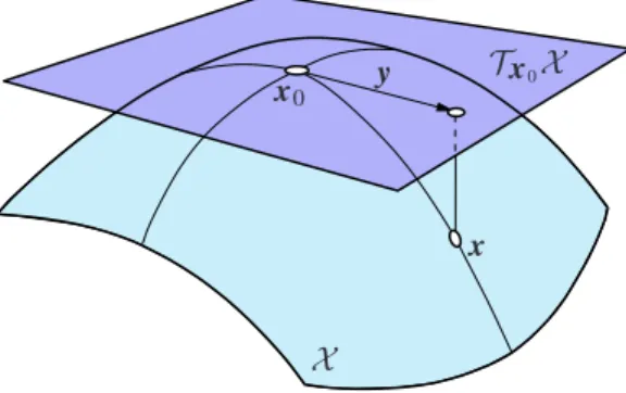
PSfrag replacements X x x0 y Tx 0X
Fig. 1. The tangent space parameterization.
coordinates [2]. The route taken in this paper is robust to such singularities because, as we shall see, we employ a time-varying parameterization of x that is always well-defined.
IV. Stabilization at a Fixed Point
Consider the reference trajectory to be x0(t) = x0 ∀t,
where x0 is a fixed point of x˙ = g(x,u) for u = u0,
i.e., g(x0,u0) = 0. We propose to use the tangent space
local parametrization to find a set of minimal coordinates and then apply LQR techniques using such coordinates. Let the tangent space of X at x0 be
Tx
0X ={x˙ ∈R
2nq :F
x(x0)x˙ =0}. (15)
The tangent space can be used to define a local diffeomor-phismϕfrom an open neighborhood ofx0inX to and open
set ofRdX. The mapy
=ϕ(x)provides the local coordinates,
or parameters, of x. This map is obtained by projecting x orthogonally to Tx0X [Fig. 1]:
y=U⊤x,¯ (16)
where U is a 2nq×dX matrix whose columns provide an
orthonormal basis of Tx0X, i.e.,U⊤
U=IdX, where IdX is
the identity matrix of size dX. This basis can be computed
efficiently using the QR decomposition of Fx at x0. Since
the map ϕ is a diffeomorphism, its inverse map ψ = ϕ−1 exists and is implicitly determined by the system of nonlinear equations
F(x)=0,
U⊤x¯−y=0, (17)
which, for a given y ∈RdX, can be solved for x using the
Newton-Raphson method (if x is close to x0).
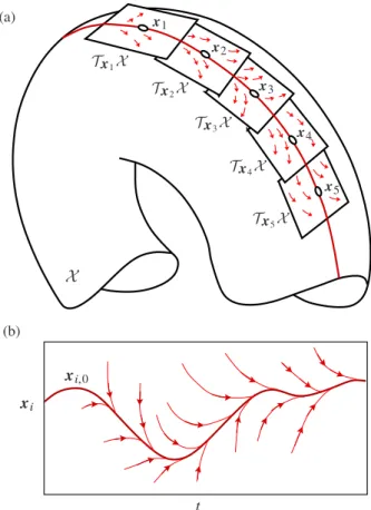
The time derivative of Eq. (16) gives the expression of the vector field defined by Eq. (6) in local coordinates of the tangent space [Fig.2(a)]:
˙
y=U⊤x˙ =U⊤g(ψ(y),u)=g˜(y,u). (18)
The resulting system may not be stable at the fixed point and thus, our goal is to find a feedback law to stabilize it [Fig.2(b)].
Since we wish asymptotic convergence to the fixed point, we are in the context of infinite-horizon optimal control. Therefore, we set the terminal timetf of the cost in Eq. (11)
to infinity. Moreover, by using y =U⊤ x, this cost can be¯ rewritten in terms of the local coordinates y:
J= Z ∞ 0 f y⊤(t)Q y˜ (t)+u¯⊤(t)Ru¯(t)gdt, (19) where Q˜ =U⊤QU.
To obtain an LQR solution, we linearize Eq. (18) around the fixed point to get a linear time-invariant system in tangent space coordinates, ˙ y=Ay˜ +B˜u,¯ (20) where ˜ A= ∂ ˜ g ∂y =U ⊤ ∂g ∂x ∂ψ(y) ∂y , and ˜ B= ∂ ˜ g ∂u =U ⊤ ∂g ∂u.
Note that ∂ψ∂(yy) can be computed in closed form. Consider the mapping
y=ϕ(x)=U⊤(x−x0). (21)
Lets now use the inverse mapping x = ψ(y) to rewrite Eq. (21) as
y=U⊤ ψ(y)−x0. (22)
If we compute the partial derivative of both side of Eq. (22) with respect to y, we have
IdX =U
⊤∂ψ(y)
∂y . (23)
Thus, ∂ψ∂(yy) must beU.
From the theory of Section III, the optimal control that minimizes the cost in Eq. (19) for the system in Eq. (20) is given by
u=π(y)=u0−K y,˜ (24)
which can be written in terms of the x variables as u=π(x)=u0−K U˜ ⊤x¯. (25)
Since we are solving an infinite horizon control problem, the solution of Eq. (14) reduces to the algebraic Riccati equation [14]
0=SA˜+A˜⊤S−SBR˜ −1B˜⊤S+Q,˜ (26)
which can be solved using generalized eigenvalue meth-ods [16].
V. Trajectory Stabilization
Now consider the general case of stabilizing an arbitrary trajectory x0(t),u0(t). Since this trajectory is now
time-varying, the tangent space basis U(t) and the mappings ψ(y,t)andϕ(x,t) are also time-varying along x0(t).
PSfrag replacements (a) (b) X Tx0X Tx 0X (y space) (y space) 0 0 x0
Fig. 2. (a) A vector fieldx˙=g(x,u)onX can be locally expressed in tangent-space coordinates. The field is action varying, but we draw it for a given value ofuonly. (b) If, as in (a),x0is a fixed point for someu=u0, we can design a feedback law to stabilize the system atx0.
As in the previous section, we also write the vector field in local coordinates, which can be done by differentiating Eq. (16): ˙ y=U˙⊤(t)x¯ +U⊤(t)x˙¯ =U˙⊤(t) ψ(y,t)−x0(t)+ U⊤(t) g(ψ(y,t),u)−g(x 0(t),u0(t)) =g˜(y,u,t). (27)
Note that the resulting vector field is now action- and time-varying [Fig. 3(a)], and our goal is to stabilize this system to make it convergent to the desired trajectory [Fig. 3(b)].
Noting that the terminal timetf is the trajectory time, we rewrite the finite-horizon cost in local coordinates as
J= Z tf 0 f y⊤(t)Q˜(t)y(t)+u¯⊤(t)Ru¯(t)gdt. (28) where Q˜(t) =U⊤(t)Q U(t).
Now we linearize Eq. (27) about x0(t),u0(t) to obtain:
˙ y=A˜(t)y+B˜(t)u,¯ (29) PSfrag replacements (a) (b) Tx1X Tx2X Tx3X Tx4X Tx5X x1 x2 x3 x4 x5 X t xi,0 xi
Fig. 3. (a) The linearization of the system along a trajectory yields a time (and action) varying vector field. At each time, the field is drawn for a single value ofu only. (b) Our goal is to design a feedback law stabilizing the system along the desired state-time trajectory.
where ˜ A(t)=∂g˜ ∂y =U˙ ⊤ (t) ∂ψ(y,t) ∂y +U ⊤(t) ∂g ∂xU(t) and ˜ B(t)= ∂ ˜ g ∂u =U ⊤ (t) ∂g ∂u. Note that ∂ψ∂(yy,t) =U(t).
The tangent space basis U(t) could be computed from a
QR decomposition of Fx(t). However, this approach does not guarantee that the time-varying basis is continuous, which is needed to obtain U˙(t). Therefore, both U(t) and
˙
U(t) can be computed considering the following identities: U⊤(t)U(t)=I,
F x(t)U(t)=0, (30)
which can be differentiated to obtain: ˙
U⊤(t)U(t)+U⊤(t)U˙(t)=0, (31)
˙
F x(t)U(t)+F x(t)U˙(t)=0. (32)
From Eq. (32),U˙(t) can be isolated to obtain ˙
U(t)=−F+
x(t)F x˙ (t)U(t), (33) where F+
x(t) is the pseudoinverse ofF x(t), which requires the Jacobian F x(t) to be full rank ∀t. Then, U(t) can be
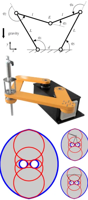
PSfrag replacements q1 q2 q3 q4 q5 gravity x y E d L L l l PSfrag replacements q1 q2 q3 q4 q5 gravity x y E d L l PSfrag replacements q1 q2 q3 q4 q5 gravity x y E d L l
Fig. 4. Top: Geometry of a five-bar robot. Middle: the RAPI-MOD model by Gridbot technologies. Bottom: the workspace of the robot (in grey) and its forward singularity locus (in red). Two near-singular configurations are shown in the right.
obtained integrating Eq. (33) from U(0) enforcing Eq. (30) at each integration step.
Then, from the results in Section III, the optimal control that minimizes the cost in Eq. (28) for the system in Eq. (29) is given by
u(t)=π(y,t)=u0(t)−K˜(t)y, (34)
which in terms of the x variables results in
u=π(x,t)=u0(t)−K˜(t)U⊤(t)x¯. (35) PSfrag replacements E rr or [r ad ] t[s] Ext. Force Fext P E
Fig. 5. Left: A weight stabilization task. The robot has to keep an end-effector load at position E, counteracting bounded disturbances applied (Fe x t). Right: The error responses of all joints angles shown over time, drawn with different colors. The force disturbances are applied (and kept constant) during the grey time windows. An animation of the motion can be seen inyoutu.be/LNoFYAW209Q.
VI. Test Cases
We next illustrate the performance of the previous LQR controllers in a five-bars robot with the geometry shown in Fig.4(top). The anglesq1 andq5 are actuated, which allow
us to control the positionE of the end-effector. The remain-ing anglesq2,q3, andq4are passive. Various versions of this
robot have been used both in research and industry [17], [18]. Fig. 4 (middle), for example, shows the RAPI-MOD model from Gridbot technologies. In our version, the base distance is d =0.6472 [m], and the proximal and distal link lengths areL =1.14[m] andl =0.9[m]. With these dimensions, the workspace of pointEis the grey area of Fig.4(bottom-left). This figure also shows the positions ofEfor which a forward singularity is encountered (in red). We recall from [17] that such singularities appear wheneverq3 is either 0or π.
Because of the complications introduced by forward sin-gularities, programmers tend to restrict the motion of these robots to singularity-free regions of the workspace [19]. From Fig.4(bottom) it is obvious, however, that the motion capabilities would be further enlarged if singularity-crossing motions could be controlled. The following examples show that the proposed LQR controller is successful in achieving such goal. In all examples, the mass of each link is0.5[kg] and the end-effector is transporting a load of 1 [kg]. The moments of inertia of the proximal and distal links (with respect to their center of gravity) are of0.0541[kg·m2] and 0.0338 [kg·m2], respectively.
A. Weight Stabilization at a Forward Singularity
In this example, the robot has to keep its load of 1 [Kg] at the upright configuration of Fig. 5 (left). The two distal links are coincident in such a pose. Thus the robot will move very close to the singularity all of the time, which renders computed-torque methods inapplicable to the situation. The task is difficult because the upper two links can fall down by gravity under the slightest disturbances. Without feedback, therefore, the robot is at an unstable fixed point, and thus the example is ideal to test the controller of SectionIV.
To show the robustness of this controller, we simulate the effect of an horizontal disturbance force Fext applied
PSfrag replacements
1 2 3 4 5 6 7
8 9 10 11 12 13 14
Fig. 6. A weight-throwing task. The robot picks an object in a lower position (snapshot 1) and performs successive swing-up motions to throw it from an upper position (snapshot 14). The robot crosses the forward singularity twice (snapshots 4 and 9). An animation of the motion can be seen in
youtu.be/LNoFYAW209Q. PSfrag replacements q [r ad ] q [r ad ] t[s] t[s] q1 q2 q3 q4 q5 Ext. Force Singularity q0
Fig. 7. Comparison of the LQR controller (upper plot) with a standard CT controller (lower plot) in a trajectory stabilization task under disturbances and singularity crossing. An animation of the motion can be seen in
youtu.be/LNoFYAW209Q.
to pointE every3 seconds. Every disturbance is maintained during 0.2seconds, and its magnitude is randomly selected in the range (−15,0)[N]. Fig.5 (right) shows the evolution
of all joint angle errors during the application of these disturbances, which occur at the time windows shown in grey. As we see, the LQR controller compensates the disturbances and returns the robot to the desired position in all cases. See
youtu.be/LNoFYAW209Qfor an animation of the task.
The convergence rate of the controller can be tunned by changing theQandRmatrices of Eq. (11). The plot of Fig.5 was obtained with
Q= " kqI5 0 0 kvI5 # (36) and R=kuI2, (37)
where kq = 300, kv = 10 and ku = 2. The size of these
matrices agrees with the fact that q = (q1, . . . ,q5) in this
robot (and thusnq =5) and only two joints are actuated (i.e.
na=2).
B. A Weight Throwing Task
We next compare the performance of the LQR and CT controllers on tracking a trajectory across forward singular-ities. The reference trajectory x0(t) and its action history
u0(t) have been obtained with the planner in [8], and
correspond to a weight-throwing task illustrated in Fig. 6. The robot has to pick a heavy ball in the lowest position of its workspace (first snapshot) and has to successively increase its velocity so as to throw it from an upper position (last snapshot). The robot goes twice across forward singularities (snapshots 4 and 9). Thus its control may be loosed at such configurations.
The tracking results of the LQR and CT controllers are compared in Fig.7. In both cases, the robot is subject to the same disturbances. These are applied to the end-effector, and take place during the grey time windows indicated. The time instants in which the singularities are crossed are indicated with a black vertical line. The reference trajectories for all anglesqi are drawn with discontinuous lines. As we see, the CT controller can counteract the applied disturbances before meeting the first singularity. At the forward singularity, however, the inverse dynamic problem produces unbounded torques. The control of the robot is lost, and the rest of the trajectory cannot be tracked anymore. The CT controller
has been implemented in the active joint space, and thus q1(t) and q5(t) can reliably be tracked, but note that the
remaining angles evolve differently because of configuration-space bifurcations. On the contrary, the LQR controller is quite robust to disturbances and singularity crossings. Even if an external force is applied right before the second singularity, the LQR controller is able to converge to the desired trajectory. A video showing the two experiments can be found in youtu.be/LNoFYAW209Q.
VII. Conclusions
This paper proposes the adaptation of an LQR controller to treat the closed-kinematic chains that arise in parallel robots. We use the tangent space local parametrization to find a set of minimal coordinates for the system in order to formulate the LQR controller in such coordinates. With this technique, we are able to stabilize both a fixed point and a preplanned trajectory. This controller can cope with forward singularities, whereas existing CT controllers cannot. Specifically, we are able to stabilize these singularity under significant disturbances at the end-effector. In contrast, the CT method produces unbounded torque at these points, which results in a trajectory that cannot be fully tracked anymore once the singularity is reached.
Our current efforts are focused on the implementation and validation of the proposed approach in a real robot.
References
[1] L.-W. Tsai, Robot Analysis: the Mechanics of Serial and Parallel Manipulators. Wiley-Interscience, 1999.
[2] O. Bohigas, M. Manubens, and L. Ros,Singularities of robot mech-anisms: numerical computation and avoidance path planning, ser. Mechanisms and Machine Science. Springer, 2016, vol. 41. [3] ——, “Singularities of non-redundant manipulators: A short account
and a method for their computation in the planar case,”Mechanism and Machine Theory, vol. 68, pp. 1–17, 2013.
[4] S. Briot and V. Arakelian, “Optimal force generation in parallel manip-ulators for passing through the singular positions,”The International Journal of Robotics Research, vol. 27, no. 8, pp. 967–983, 2008. [5] C. K. Kevin Jui and Q. Sun, “Path tracking of parallel manipulators
in the presence of force singularity,” Journal of dynamic systems, measurement, and control, vol. 127, no. 4, pp. 550–563, 2005. [6] S. K. Ider, “Inverse dynamics of parallel manipulators in the presence
of drive singularities,”Mechanism and Machine Theory, vol. 40, no. 1, pp. 33–44, 2005.
[7] M. Özdemir, “Removal of singularities in the inverse dynamics of parallel robots,”Mechanism and Machine Theory, vol. 107, pp. 71– 86, 2017.
[8] R. Bordalba, L. Ros, and J. M. Porta, “Randomized Kinodynamic Planning for Constrained Systems,” inIEEE International Conference on Robotics and Automation, 2018.
[9] R. Bordalba, J. M. Porta, and L. Ros, “Randomized kinodynamic planning for cable-suspended parallel robots,” inCable-Driven Parallel Robots. Springer, 2018, pp. 195–206.
[10] F. Aghili, “A unified approach for inverse and direct dynamics of constrained multibody systems based on linear projection operator: ap-plications to control and simulation,”IEEE Transactions on Robotics, vol. 21, no. 5, pp. 834–849, 2005.
[11] R. B. Hill, D. Six, A. Chriette, S. Briot, and P. Martinet, “Crossing type 2 singularities of parallel robots without pre-planned trajectory with a virtual-constraint-based controller,” inIEEE International Conference on Robotics and Automation (ICRA), 2017, pp. 6080–6085. [12] M. Posa, S. Kuindersma, and R. Tedrake, “Optimization and
stabi-lization of trajectories for constrained dynamical systems,” inIEEE International Conference on Robotics and Automation, 2016, pp. 1366–1373.
[13] S. Mason, N. Rotella, S. Schaal, and L. Righetti, “Balancing and walking using full dynamics lqr control with contact constraints,” in Humanoid Robots (Humanoids), 2016 IEEE-RAS 16th International Conference on, 2016, pp. 63–68.
[14] F. L. Lewis, D. Vrabie, and V. L. Syrmos,Optimal control. John Wiley & Sons, 2012.
[15] F. A. Potra and J. Yen, “Implicit numerical integration for Euler-Lagrange equations via tangent space parametrization,” Journal of Structural Mechanics, vol. 19, no. 1, pp. 77–98, 1991.
[16] W. F. Arnold and A. J. Laub, “Generalized eigenproblem algorithms and software for algebraic Riccati equations,”Proceedings of the IEEE, vol. 72, no. 12, pp. 1746–1754, 1984.
[17] F. Bourbonnais, P. Bigras, and I. A. Bonev, “Minimum-time trajectory planning and control of a pick-and-place five-bar parallel robot,” IEEE/ASME Transactions on Mechatronics, vol. 20, no. 2, pp. 740– 749, 2015.
[18] “RAPI-MOD: Ultrafast scara robot.” [Online]. Available:
http://gridbots.com/rapi_mov.html
[19] R. Bordalba, L. Ros, and J. M. Porta, “Randomized planning of dynamic motions avoiding forward singularities,” inAdvances in Robot Kinematics, 2018, pp. 170–178.