HSC/10/04
HSC Research Rep
ort
Ruin Probability in Finite
Time
Krzysztof Burnecki*
Marek Teuerle*
* Hugo Steinhaus Center, Wrocław University of
Technology, Poland
Hugo Steinhaus Center
Wrocław University of Technology
Wyb. Wyspiańskiego 27, 50-370 Wrocław, Poland
http://www.im.pwr.wroc.pl/~hugo/
Ruin Probability in Finite
Time
1
Krzysztof Burnecki
2and Marek Teuerle
2Abstract:
The ruin probability in finite time can only be calculated analytically for
a few special cases of the claim amount distribution. The most classic example is
discussed in Section 1.2. The value can always be computed directly using Monte
Carlo simulations, however, this is usually a time-consuming procedure. Thus,
finding a reliable approximation is really important from a practical point of view.
The most important approximations of the finite time ruin probability are
presented in Section 1.3. They are further illustrated in Section 1.4 using the
Danish fire losses dataset, which concerns major fire losses in profits that
occurred between 1980 and 2002 and were recorded by Copenhagen Re.
Keywords:
Insurance risk model; Ruin probability; Segerdahl approximation; De
Vylder approximation; Diffusion approximation; Brownian motion; Levy motion
JEL:
C15, C46, C63, G22, G32
1
Chapter prepared for the 2
ndedition of
Statistical Tools for Finance and Insurance
, P.Cizek,
W.Härdle, R.Weron (eds.), Springer-Verlag,
forthcoming
in 2011
.
2
1 Ruin probability in finite time
Krzysztof Burnecki and Marek Teuerle
1.1
Introduction
In examining the nature of the risk associated with a portfolio of business, it is often of interest to assess how the portfolio may be expected to perform over an extended period of time. One approach involves the use of ruin theory (Panjer and Willmot, 1992). Ruin theory is concerned with the excess of the income (with respect to a portfolio of business) over the outgo, or claims paid. This quantity, referred to as insurer’s surplus, varies in time. Specifically, ruin is said to occur if the insurer’s surplus reaches a specified lower bound, e.g. minus the initial capital. One measure of risk is the probability of such an event, clearly reflecting the volatility inherent in the business. In addition, it can serve as a useful tool in long range planning for the use of insurer’s funds.
We recall from Chapter?? that the classical risk process{Rt}t≥0 is given by
Rt=u+ct− Nt X
i=1
Xi,
where the initial capital of the insurance company is denoted byu, the homoge-neous Poisson process (HPP)Nt with intensity (rate)λdescribes the number
of claims in (0, t] interval and claim severities are random, given by i.i.d. non-negative sequence{Xk}∞k=1with mean valueµand varianceσ2, independent of
Nt. The insurance company receives a premium at a constant ratec per unit
time, wherec= (1 +θ)λµandθ >0 is called the relative safety loading. We define the claim surplus process{St}t≥0 as
St=u−Rt= Nt X
i=1
and the time to ruin asτ(u) = inf{t≥0 :Rt<0}= inf{t≥0 :St> u}. Let
L= sup0≤t<∞{St} andLT = sup0≤t<T{St}. The ruin probability in infinite
time, i.e. the probability that the capital of an insurance company ever drops below zero can be then written as
ψ(u) = P(τ(u)<∞) = P(L > u). (1.1) We note that the above definition implies that the relative safety loadingθhas to be positive, otherwisec would be less than λµand thus with probability 1 the risk business would become negative in infinite time. The ruin probability in finite timeT is given by
ψ(u, T) = P(τ(u)≤T) = P(LT > u). (1.2)
From a practical point of view, ψ(u, T), where T is related to the planning horizon of the company, is regarded as more interesting than ψ(u). Most in-surance managers will closely follow the development of the risk business and increase the premium if the risk business behaves badly. The planning horizon may be thought of as the sum of the following: the time until the risk business is found to behave “badly”, the time until the management reacts and the time until a decision of a premium increase takes effect. Therefore, in non-life in-surance, it may be natural to regardT equal to four or five years as reasonable (Grandell, 1991).
Let us now analyze the finite-time ruin probability for the probably most practical generalization of the classical risk process, where the occurrence of the claims is described by the non-homogeneous Poisson process (NHPP), see Chapter??. It can be proved that switching from HPP to NHPP results only in altering the time horizon T. This stems from the following fact. Consider a risk process ˜Rt driven by a non-homogeneous Poisson process ˜Nt with the
intensity functionλ(t), namely ˜ Rt=u+ (1 +θ)µ Z t 0 λ(s)ds− ˜ Nt X i=1 Xi. (1.3)
Define now Λt = R0tλ(s)ds and Rt = ˜R(Λ−t1). Then the counting process
Nt= ˜N(Λ−t1) is a standard Poisson process, and therefore,
˜ ψ(u, T) = P inf 0<t≤T( ˜Rt)<0 = P inf 0<t≤ΛT (Rt)<0 =ψ(u,ΛT). (1.4)
1.1 Introduction 3
The time scale defined by Λ−1
t is called the operational time scale.
The ruin probability in finite time can only be calculated analytically for a few special cases of the claim amount distribution. The most classic example is discussed in Section 1.2. The value ofψ(u, T) can always be computed di-rectly using Monte Carlo simulations, however, this is usually a time-consuming procedure. Thus, finding a reliable approximation is really important from a practical point of view. The most important approximations of the finite time ruin probability are presented in Section 1.3. They are further illustrated in Section 1.4 using the Danish fire losses dataset, introduced in Chapter??, which concerns major fire losses in profits that occurred between 1980 and 2002 and were recorded by Copenhagen Re.
We note that ruin theory has been also recently employed as an interesting tool in operational risk (Degen, Embrechts, and Lambrigger, 2007; Kaishev, Dimitrova, and Ignatov, 2008). In the view of the data already available on op-erational risk, ruin type estimates may become useful (Embrechts, Kaufmann, and Samorodnitsky, 2004).
1.1.1
Light- and heavy-tailed distributions
A distributionFX(x) is said to be light-tailed, if there exist constantsa >0,
b >0 such that ¯FX(x) = 1−FX(x)≤ae−bxor, equivalently, if there existz >0,
such thatMX(z)<∞, where MX(z) is the moment generating function, see
Chapter ??. Distribution FX(x) is said to be heavy-tailed, if for all a > 0,
b >0 ¯FX(x)> ae−bx,or, equivalently, if ∀z > 0MX(z) =∞. We study here
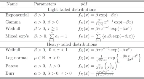
eight claim size distributions, as listed in Table 1.1.
In the case of light-tailed claims the adjustment coefficient (also called the Lundberg exponent) plays a key role in calculating the ruin probability. Let γ= supz{MX(z)}<∞and letR be a positive solution of the equation:
1 + (1 +θ)µR=MX(R), R < γ. (1.5)
If there exists a non-zero solutionR to the above equation, we call it an ad-justment coefficient. Clearly, R = 0 satisfies equation (1.5), but there may exist a positive solution as well (this requires thatX has a moment generating function, thus excluding distributions such as Pareto and the log-normal). To see the plausibility of this result, note thatMX(0) = 1,MX′ (z)<0,M
′′
X(z)>0
andMX′ (0) =−µ. Hence, the curves y =MX(z) and y = 1 + (1 +θ)µz may
Table 1.1: Typical claim size distributions. In all casesx≥0. Name Parameters pdf Light-tailed distributions Exponential β >0 fX(x) =βexp(−βx) Gamma α >0,β >0 fX(x) = β α Γ(α)xα−1exp(−βx) Weibull β >0,τ≥1 fX(x) =βτ xτ−1exp(−βxτ) Mixed exp’s βi >0, n P i=1 ai= 1 fX(x) = n P i=1{ aiβiexp(−βix)} Heavy-tailed distributions Weibull β >0, 0< τ <1 fX(x) =βτ xτ−1exp(−βxτ) Log-normal µ∈R, σ >0 fX(x) = √1 2πσxexp n −(ln2xσ−2µ)2 o Pareto α >0, λ >0 fX(x) = λα+x λ λ+x α Burr α >0,λ >0,τ >0 fX(x) = ατ λ αxτ−1 (λ+xτ)α+1 0 R 0.95 1 1.05 1.1 1.15 1.2 1.25 1.3 1.35 1.4 z y y=1+(1+θ)µ z M X(z)
Figure 1.1: Illustration of the existence of the adjustment coefficient.
1.2 Exact ruin probabilities in finite time 5
An analytical solution to equation (1.5) exists only for few claim distributions. However, it is quite easy to obtain a numerical solution. The coefficient R satisfies the inequality:
R < 2θµ
µ(2), (1.6)
whereµ(2) = E(X2
i), see Asmussen (2000). LetD(z) = 1 + (1 +θ)µz−MX(z).
Thus, the adjustment coefficient R > 0 satisfies the equation D(R) = 0. In order to get the solution one may use the Newton-Raphson formula
Rj+1=Rj−
D(Rj)
D′(Rj), (1.7)
with the initial condition R0 = 2θµ/µ(2), where D′(z) = (1 +θ)µ−MX′ (z).
Moreover, if it is possible to calculate the third raw momentµ(3), we can obtain
a sharper bound than (1.6) (Panjer and Willmot, 1992):
R < 12µθ
3µ(2)+p
9(µ(2))2+ 24µµ(3)θ,
and use it as the initial condition in (1.7).
1.2
Exact ruin probabilities in finite time
We are now interested in the probability that the insurer’s capital as defined by (1.1) remains non-negative for a finite periodT. We assume that the claim counting processNtis a homogeneous Poisson process (HPP) with rateλ, and
consequently, the total claims (aggregate loss) process is a compound Poisson process. Premiums are payable at ratec per unit time. We recall that if Nt
is a non-homogeneous Poisson process, which will be the case for all numerical examples, then it is enough to rescale the time horizonT for the ruin probability obtained for the classic HPP case, see the discussion at the end of Section 1.1. In contrast to the infinite time case there is no general result for the ruin probability like the Pollaczek–Khinchin formula (Burnecki, Mi´sta, and Weron, 2005). In the literature one can only find a partial integro-differential equation which satisfies the probability of non-ruin, see Panjer and Willmot (1992). An explicit result is merely known for the exponential claims, and even is this case numerical integration is needed (Asmussen, 2000).
1.2.1
Exponential claim amounts
First, in order to simplify the formulae, let us assume that claims have the exponential distribution with β = 1 and the amount of premium is c = 1. Then
ψ(u, T) =λexp{−(1−λ)u} − 1
π Z π 0 f1(x)f2(x) f3(x) dx, (1.8) where f1(x) =λexp n 2√λTcosx−(1 +λ)T+u√λcosx−1o, (1.9) f2(x) = cos
u√λsinx−cosu√λsinx+ 2x, (1.10) and
f3(x) = 1 +λ−2 √
λcosx. (1.11)
Now, notice that the caseβ6= 1 is easily reduced to β= 1, using the formula: ψλ,β(u, T) =ψλ
β,1(βu, βT). (1.12)
Moreover, the assumptionc= 1 is not restrictive since we have
ψλ,c(u, T) =ψλ/c,1(u, cT). (1.13)
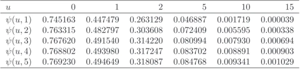
Table 1.2 shows the exact values of the ruin probability for a NHPP with the intensity rate λ(t) = 17.9937 + 7.1518t and exponential claims with β = 1.9114·10−6 (the parameters were estimated in Chapter ?? for the Danish
fire losses dataset) with respect to the initial capitaluand the time horizonT. The relative safety loadingθ is set to 30%.
1.3
Approximations of the ruin probability in finite
time
In this section, we present six different approximations. We illustrate them on a common example, namely a NHPP with the intensity rateλ(t) = 17.9937 + 7.1518t, the mixture of two exponentials claims with β1= 3.8617·10−7,β2=
1.3 Approximations of the ruin probability in finite time 7
Table 1.2: The ruin probability for a NHPP with the intensity functionλ(t) = 17.9937 + 7.1518t, exponential claims with β = 1.9114·10−6 and
θ= 0.3 (uin DKK millions). u 0 1 2 5 10 15 ψ(u,1) 0.745163 0.447479 0.263129 0.046887 0.001719 0.000039 ψ(u,2) 0.763315 0.482797 0.303608 0.072409 0.005595 0.000338 ψ(u,3) 0.767620 0.491540 0.314220 0.080994 0.007930 0.000694 ψ(u,4) 0.768802 0.493980 0.317247 0.083702 0.008891 0.000903 ψ(u,5) 0.769230 0.494649 0.318087 0.084768 0.009341 0.001029 STF2ruin02.m
for the Danish fire losses dataset) and the relative safety loading θ = 30%. Numerical comparison of the approximations is given in Section 1.4. All the formulas presented in this section assume the classic form of the risk process, however, we recall that if the processNtis a NHPP, then it is enough to rescale
the time horizonT for the ruin probability obtained for the classic HPP case.
1.3.1
Monte Carlo method
The ruin probability in finite time can always be approximated by means of Monte Carlo simulations. Table 1.3 shows the output for the with respect to the initial capitalu and the time horizon T. We note that the Monte Carlo method will be used as a reference method when comparing different finite time approximations in Section 1.4.
1.3.2
Segerdahl normal approximation
The following result due to Segerdahl (1955) is said to be a time-dependent version of the Cram´er–Lundberg approximation .
ψS(u, T) =Cexp(−Ru)Φ
T−umL
ωL√u
Table 1.3: Monte Carlo results (50 x 10000 simulations) for a NHPP with the intensity functionλ(t) = 17.9937 + 7.1518t, mixture of two exponen-tials claims withβ1= 3.8617·10−7,β2= 3.6909·10−6,a= 0.2568
andθ= 0.3 (uin DKK million). u 0 1 5 10 20 50 ψ(u,1) 0.702560 0.561842 0.302862 0.130702 0.020922 0.000062 ψ(u,2) 0.746522 0.623986 0.369984 0.193242 0.046346 0.000424 ψ(u,3) 0.758588 0.638384 0.403508 0.224844 0.064726 0.001566 ψ(u,4) 0.762924 0.646102 0.417342 0.238882 0.075002 0.001900 ψ(u,5) 0.763706 0.653820 0.419522 0.244244 0.081800 0.002300 STF2ruin03.m
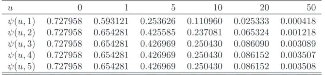
Table 1.4: The Segerdahl approximation for the same parameters as in Table 1.3. u 0 1 5 10 20 50 ψ(u,1) 0.727958 0.593121 0.253626 0.110960 0.025333 0.000418 ψ(u,2) 0.727958 0.654281 0.425585 0.237081 0.065324 0.001218 ψ(u,3) 0.727958 0.654281 0.426969 0.250430 0.086090 0.003089 ψ(u,4) 0.727958 0.654281 0.426969 0.250430 0.086152 0.003507 ψ(u,5) 0.727958 0.654281 0.426969 0.250430 0.086152 0.003508 STF2ruin04.m where C = θµ/{M′ X(R)−µ(1 +θ)}, mL = C{λMX′ (R)−1}− 1 and ω2
L = λMX′′(R)m3L. This method requires existence of the adjustment
coeffi-cient, so the moment generating function. This implies that only light-tailed distributions can be used. Numerical evidence shows that the Segerdahl ap-proximation gives the best results for large values of the initial capital u, see Asmussen (2000).
In Table 1.4 the results of the Segerdahl approximation are presented with respect to the initial capital uand the time horizon T. We can see that the
1.3 Approximations of the ruin probability in finite time 9
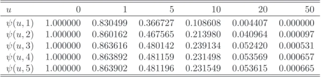
Table 1.5: The diffusion approximation by Brownian motion for the same pa-rameters as in Table 1.3. u 0 1 5 10 20 50 ψ(u,1) 1.000000 0.830499 0.366727 0.108608 0.004407 0.000000 ψ(u,2) 1.000000 0.860162 0.467565 0.213980 0.040964 0.000097 ψ(u,3) 1.000000 0.863616 0.480142 0.239134 0.052420 0.000531 ψ(u,4) 1.000000 0.863892 0.481159 0.231498 0.053569 0.000657 ψ(u,5) 1.000000 0.863902 0.481196 0.231549 0.053615 0.000665 STF2ruin05.m
approximation in the considered case yields quite accurate results for largeru’s except foru= 50 million DKK, see Table 1.3, but this effect can be explained by very small values of the probability.
1.3.3
Diffusion approximation by Brownian motion
The idea of a diffusion (weak) approximation goes back to Iglehart (1969). The first approximation we study assumes that the distribution of claim sizes be-longs to the domain of attraction of the normal law, i.e. claims are i.i.d. and have light tails. This leads to the approximation of the risk process by a diffu-sion driven by the Brownian motion. In this case one can calculate an analytical approximation formula for the ruin probability in finite time (Grandell, 1991):
ψDB(u, t) = P inf 0≤t≤T u+ (c−λµ)t−pλµ(2)B(t)<0 = = IG T µ2 c σ2 c ;−1;u|µc| σ2 c , (1.15)
whereB(t) denotes the Brownian motion,µc=λθµ,σc=λµ(2) andIG(·;ζ;u)
denotes the inverse Gaussian distribution function, namely IG(x;ζ;u) = 1−Φ u/√x−ζ√x
+ exp (2ζu) Φ −u/√x−ζ√x
. (1.16) This formula can be also obtained by matching the first two moments of the claim surplus processSt and a Brownian motion with drift (arithmetic
Brow-nian motion), and noting that such an approximation implies that the first passage probabilities are close. The first passage probability serves as the ruin probability, see Asmussen (2000). We also note that in order to apply this approximation we need the existence of the second moment of the claim size distribution.
Table 1.5 shows the results of the diffusion approximation by Brownian motion with respect to the initial capitaluand the time horizon T. The results lead to the conclusion that the approximation does not produce accurate results for such a choice of the claim size distribution. Only when u= 10 million DKK the results are acceptable, compare with the reference values in Table 1.3.
1.3.4
Corrected diffusion approximation
The idea presented in Section 1.3.3 ignores the presence of jumps in the risk process (the Brownian motion with drift can continuous trajectories). The cor-rected diffusion approximation takes this and other deficits into consideration (Asmussen, 2000). Under the assumption that c = 1, see relation (1.13), we have ψCD(u, t) =IG T δ1 u2 + δ2 u;− Ru 2 ; 1 + δ2 u , (1.17)
whereRis the adjustment coefficient,δ1=λMX′′(γ0),δ2=MX′′′(γ0)/{3MX′′(γ0)}
andγ0satisfies the equation: κ′(γ0) = 0, whereκ(s) =λ{MX(s)−1}−s.
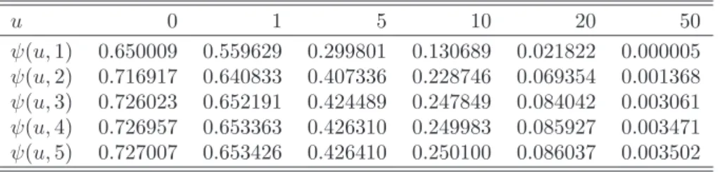
Sim-ilarly as in the Segerdahl approximation, the method requires existence of the moment generating function, so we can use it only for light-tailed distributions. In Table 1.6 the results of the corrected diffusion approximation are given with respect to the initial capitaluand the time horizon T. It turns out that corrected diffusion method gives surprisingly good results and is vastly superior to the ordinary diffusion approximation, compare with the reference values in Table 1.3.
1.3.5
Diffusion approximation by
α
-stable L´
evy motion
In this section we present theα-stable L´evy motion approximation introduced by Furrer, Michna, and Weron (1997). This is an extension of the Brownian mo-tion approximamo-tion approach. It can be applied when claims are heavy-tailed (with power-law tails), which, as the empirical results presented in Chapter??
1.3 Approximations of the ruin probability in finite time 11
Table 1.6: The corrected diffusion approximation for the same parameters as in Table 1.3. u 0 1 5 10 20 50 ψ(u,1) 0.650009 0.559629 0.299801 0.130689 0.021822 0.000005 ψ(u,2) 0.716917 0.640833 0.407336 0.228746 0.069354 0.001368 ψ(u,3) 0.726023 0.652191 0.424489 0.247849 0.084042 0.003061 ψ(u,4) 0.726957 0.653363 0.426310 0.249983 0.085927 0.003471 ψ(u,5) 0.727007 0.653426 0.426410 0.250100 0.086037 0.003502 STF2ruin06.m
We assume that the distribution of the claim sizes belongs to the domain of attraction of the stable law, that is:
1 ϕ(n) n X k=1 (Xk−µ) d →Zα,β(1), (1.18)
where ϕ(n) =L(n)n1/α for L(n) being a slowly varying function in infinity,
Zα,β(t) is theα-stable L´evy motion with scale parameter 1, skewness parameter
β, and 1< α <2 (Nolan, 2010). Ifϕ(n) =σ′n1/α, so that{X
k :k∈N}belong to the so-called normal domain
of attraction, then the diffusion approximation with α-stable L´evy motion is given by: ψDS(u, T) =P inf 0≤t≤T(u+ (c−λµ)t−σ ′λ1/αZ α,β(t))<0 , (1.19) where this probability can be calculated via Monte Carlo method by simulating trajectories ofα-stable L´evy motion.
In order to illustrate formula (1.19) we cannot consider mixture of exponentials case which was discussed in Sections 1.3.1-1.3.4 as it belongs to the domain of attraction of normal law. Let us now assume that the claim amounts are Pareto distributed with parameters 1< α′ <2 andλ′. One may check (Nolan, 2010)
that the Pareto distribution belongs to the domain of attraction of α-stable law with
Table 1.7: Diffusion approximation withα-stable L´evy motion for a NHPP with the intensity function λ(t) = 17.9937 + 7.1518t, Pareto claims with α′ = 1.3127,λ′ = 4.0588·105 andθ= 0.3 (uin DKK million). u 0 1 5 10 20 50 ψ(u,1) 0.469314 0.383986 0.232228 0.154332 0.087890 0.033532 ψ(u,2) 0.563410 0.491590 0.357850 0.280278 0.200526 0.106646 ψ(u,3) 0.605470 0.540044 0.417866 0.345702 0.268440 0.168546 ψ(u,4) 0.629782 0.568426 0.453638 0.385306 0.311520 0.212744 ψ(u,5) 0.646558 0.587962 0.478302 0.412866 0.341622 0.245320 STF2ruin07.m and σ′ =λ′ π 2Γ(α′) sin(α′π 2 ) !1/α′ =λ′ Γ(2 −α′) α′−1 cosπα′ 2 1/α′ .
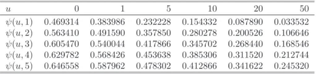
Table 1.7 depicts the results of the diffusion approximation withα-stable L´evy motion for a NHPP with the intensity rateλ(t), Pareto claims withα′,λ′with
respect to the initial capital u and the time horizon T. The relative safety loadingθ equals 30%.
1.3.6
Finite time De Vylder approximation
Let us recall the idea of the De Vylder approximation in infinite time (Burnecki, Mi´sta, and Weron, 2005): we replace the claim surplus process with the one withθ= ¯θ, λ= ¯λand exponential claims with parameter ¯β, fitting first three moments. Here, the idea is the same. First, we compute
¯ β =3µ (2) µ(3) , λ¯= 9λµ(2)3 2µ(3)2 , and θ¯= 2µµ(3) 3µ(2)2θ.
Next, we employ relations (1.12) and (1.13) and finally use the exact, exponen-tial case formula (1.8) presented in Section 1.2.1. Obviously, the method gives
1.3 Approximations of the ruin probability in finite time 13
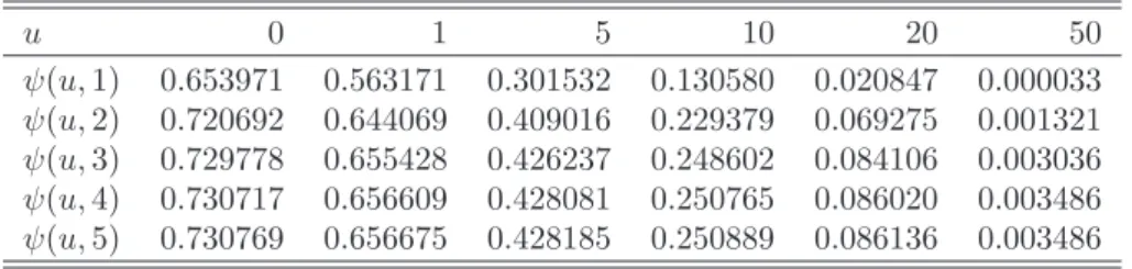
Table 1.8: The finite time De Vylder approximation for for the same parameters as in Table 1.3. u 0 1 5 10 20 50 ψ(u,1) 0.653971 0.563171 0.301532 0.130580 0.020847 0.000033 ψ(u,2) 0.720692 0.644069 0.409016 0.229379 0.069275 0.001321 ψ(u,3) 0.729778 0.655428 0.426237 0.248602 0.084106 0.003036 ψ(u,4) 0.730717 0.656609 0.428081 0.250765 0.086020 0.003486 ψ(u,5) 0.730769 0.656675 0.428185 0.250889 0.086136 0.003486 STF2ruin08.m
the exact result in the exponential case. For other claim distributions, the first three moments have to exist in order to apply the approximation.
Table 1.8 shows the results of the finite time De Vylder approximation with respect to the initial capitaluand the time horizonT. We see that this approx-imation gives even better results than the corrected diffusion approxapprox-imation, compare with the reference values presented in Table 1.3.
Table 1.9 shows which approximation can be used for each claim size distribu-tion. Moreover, the necessary assumptions on the distribution parameters are presented.
Table 1.9: Approximations and their range of applicability Distrib. Exp. Gamma Wei- Mix. Log- Pareto Burr
Method bull Exp. normal
Monte Carlo + + + + + + + Segerdahl + + – + – – – Brown. diff. + + + + + α >2 ατ >2 Corr. diff. + + – + – – – Stable diff. – – – – – α <2 ατ <2 Fin. De Vylder + + + + + α >3 ατ >3
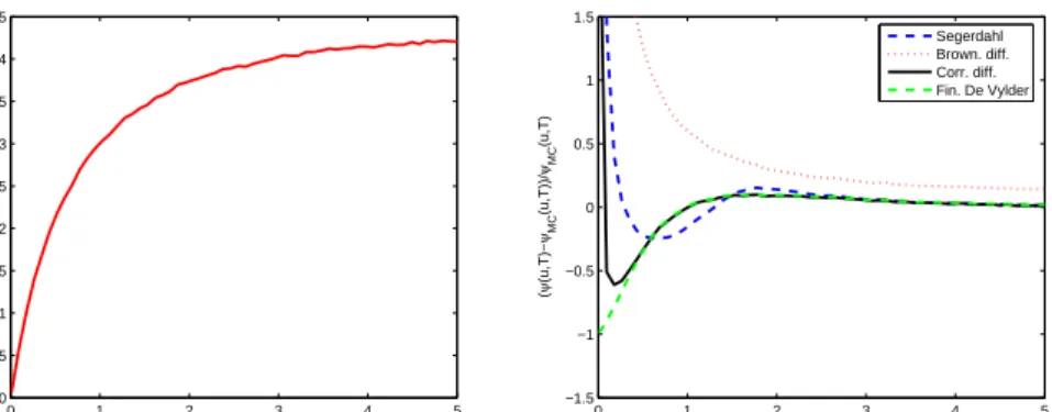
0 3 6 9 12 15 18 21 24 27 30 0 0.1 0.2 0.3 0.4 0.5 0.6 0.7 0.8 u (DKK million) ψ (u,T) 0 3 6 9 12 15 18 21 24 27 30 −1.5 −1 −0.5 0 0.5 1 1.5 u (DKK million) ( ψ (u,T)− ψMC (u,T))/ ψMC (u,T) Segerdahl Brown. diff. Corr. diff. Fin. De Vylder
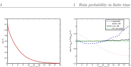
Figure 1.2: The reference ruin probability obtained via Monte Carlo simula-tions (left panel), the relative error of the approximasimula-tions (right panel). The mixture of two exponentials case with T fixed and u varying.
STF2ruin09.m
1.4
Numerical comparison of the finite time
approximations
Now, we will illustrate all six approximations presented in Section 1.3. We consider three claim amount distributions which were best fitted to the Danish fire losses data in Chapter ??, namely the mixture of two exponentials (a running example in Section 1.3), log-normal and Pareto distributions. The parameters of the distributions are: β1 = 3.8617·10−7, β2 = 3.6909·10−6,
a= 0.2568 (mixture),µ= 12.5247,σ2= 1.5384 (log-normal), andα= 1.3127,
λ= 4.0588·105 (Pareto). The ruin probability will be depicted as a function
ofu, ranging from 0 to 30 million DKK, with fixed T = 1 or with fixed value of u = 5 million DKK and varying T from 0 to 5 years. The relative safety loading is set to 30%. All figures have the same form of output. In the left panel, the reference ruin probability values obtained via 10 x 10000 Monte Carlo simulations are presented. The right panel depicts the relative error with respect to the reference values.
1.4 Numerical comparison of the finite time approximations 15 0 1 2 3 4 5 0 0.05 0.1 0.15 0.2 0.25 0.3 0.35 0.4 0.45 T (years) ψ (u,T) 0 1 2 3 4 5 −1.5 −1 −0.5 0 0.5 1 1.5 T (years) ( ψ (u,T)− ψMC (u,T))/ ψMC (u,T) Segerdahl Brown. diff. Corr. diff. Fin. De Vylder
Figure 1.3: The reference ruin probability obtained via Monte Carlo simula-tions (left panel), the relative error of the approximasimula-tions (right panel). The mixture of two exponentials case with ufixed and T varying.
STF2ruin10.m
and 1.3 the Brownian motion diffusion and Segerdahl approximations almost for all values of u and T give highly incorrect results. Corrected diffusion and finite time De Vylder approximations yield acceptable errors, which are generally below 10%.
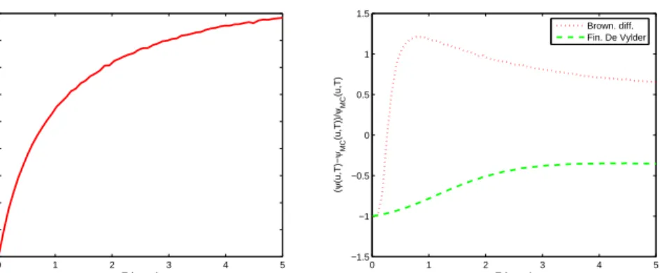
In the case of log-normally distributed claims, we can only apply two approx-imations: diffusion by Brownian motion and finite time De Vylder, see Table 1.9. Figures 1.4 and 1.5 depict the reference ruin probability values obtained via Monte Carlo simulations and the relative errors with respect to the refer-ence values. Again, the finite time De Vylder approximation works better than the diffusion approximation, but, in general, the errors are not acceptable. Finally, we take into consideration the Pareto claim size distribution. Fig-ures 1.6 and 1.7 depict the reference ruin probability values and the relative errors with respect to the reference values for theα-stable L´evy motion diffu-sion approximation (we cannot apply finite time De Vylder approximation as α <3). We see that the error is quite low for high values ofT.
0 3 6 9 12 15 18 21 24 27 30 0 0.1 0.2 0.3 0.4 0.5 0.6 0.7 0.8 u (DKK million) ψ (u,T) 0 3 6 9 12 15 18 21 24 27 30 −1.5 −1 −0.5 0 0.5 1 1.5 u (DKK million) ( ψ (u,T)− ψMC (u,T))/ ψMC (u,T) Brown. diff. Fin. De Vylder
Figure 1.4: The reference ruin probability obtained via Monte Carlo simula-tions (left panel), the relative error of the approximasimula-tions (right panel). The log-normal case withT fixed anduvarying.
STF2ruin11.m 0 1 2 3 4 5 0 0.05 0.1 0.15 0.2 0.25 0.3 0.35 0.4 0.45 T (years) ψ (u,T) 0 1 2 3 4 5 −1.5 −1 −0.5 0 0.5 1 1.5 T (years) ( ψ (u,T)− ψMC (u,T))/ ψMC (u,T) Brown. diff. Fin. De Vylder
Figure 1.5: The reference ruin probability obtained via Monte Carlo simula-tions (left panel), the relative error of the approximasimula-tions (right panel). The log-normal case withufixed andT varying.
1.4 Numerical comparison of the finite time approximations 17 0 3 6 9 12 15 18 21 24 27 30 0 0.1 0.2 0.3 0.4 0.5 0.6 0.7 0.8 u (DKK million) ψ (u,T) 0 3 6 9 12 15 18 21 24 27 30 −1.5 −1 −0.5 0 0.5 1 1.5 u (DKK million) ( ψ (u,T)− ψMC (u,T))/ ψMC (u,T) Stable diff.
Figure 1.6: The reference ruin probability obtained via Monte Carlo simula-tions (left panel), the relative error of the approximation with α-stable L´evy motion (right panel). The Pareto case withT fixed and uvarying. STF2ruin13.m 0 1 2 3 4 5 0 0.05 0.1 0.15 0.2 0.25 0.3 0.35 0.4 0.45 T (years) ψ (u,T) 0 1 2 3 4 5 −1.5 −1 −0.5 0 0.5 1 1.5 T (years) ( ψ (u,T)− ψMC (u,T))/ ψMC (u,T) Stable diff.
Figure 1.7: The reference ruin probability obtained via Monte Carlo simula-tions (left panel), the relative error of the approximation with α-stable L´evy motion (right panel). The Pareto case withufixed and T varying.
Bibliography
Asmussen, S. (2000). Ruin Probabilities, World Scientific, Singapore.
Burnecki, K. (2000). Self-similar processes as weak limits of a risk reserve process,Probab. Math. Statist.20(2): 261-272.
Burnecki, K., Mi´sta, P., and Weron, A. (2005). Ruin Probabilities in Finite and Infinite Time,inP. Cizek, W. H¨ardle, and R. Weron (eds.)Statistical
Tools for Finance and Insurance, Springer, Berlin, 341-379.
Burnecki, K., Mi´sta, P., and Weron, A. (2005). What is the best approximation of ruin probability in infinite time?, Appl. Math. (Warsaw) 32(2): 155-176.
Degen, M., Embrechts, P., and Lambrigger, D.D. (2007). The quantitative modeling of operational risk: between g-and-h and EVT, Astin Bulletin
37(2): 265-291.
Embrechts, P., Kaufmann, R., and Samorodnitsky, G. (2004). Ruin Theory Revisited: Stochastic Models for Operational Risk,in C. Bernadell et al (eds.) Risk Management for Central Bank Foreign Reserves, European Central Bank, Frankfurt a.M., 243-261.
Furrer, H., Michna, Z., and Weron, A. (1997). Stable L´evy motion approxima-tion in collective risk theory,Insurance Math. Econom. 20: 97–114. Grandell, J. (1991). Aspects of Risk Theory, Springer, New York.
Iglehart, D. L. (1969). Diffusion approximations in collective risk theory,
Jour-nal of Applied Probability6: 285–292.
Kaishev, V.K., Dimitrova, D.S. and Ignatov, Z.G. (2008). Operational risk and insurance: a ruin-probabilistic reserving approach,Journal of Operational Risk3(3): 39–60.
Nolan, J.P. (2010). Stable Distributions - Models for Heavy Tailed Data, Birkhauser, Boston, In progress, Chapter 1 online at academic2.american.edu/∼jpnolan.
Panjer, H.H. and Willmot, G.E. (1992). Insurance Risk Models, Society of Actuaries, Schaumburg.
Segerdahl, C.-O. (1955). When does ruin occur in the collective theory of risk?,