Singapore Management University
Institutional Knowledge at Singapore Management University
Research Collection School Of Economics
School of Economics
9-2014
Testing Conditional Independence via Empirical
Likelihood
Liangjun SU
Singapore Management University, [email protected]
Halbert WHITE
University of Southern California
DOI:https://doi.org/10.1016/j.jeconom.2014.04.006
Follow this and additional works at:
https://ink.library.smu.edu.sg/soe_research
Part of the
Econometrics Commons
This Journal Article is brought to you for free and open access by the School of Economics at Institutional Knowledge at Singapore Management University. It has been accepted for inclusion in Research Collection School Of Economics by an authorized administrator of Institutional Knowledge at Singapore Management University. For more information, please [email protected].
Citation
SU, Liangjun and WHITE, Halbert. Testing Conditional Independence via Empirical Likelihood. (2014).Journal of Econometrics. 182, (1), 27-44. Research Collection School Of Economics.
Testing Conditional Independence via Empirical Likelihood
∗
Liangjun Su
aand Halbert White
ba
School of Economics, Singapore Management University, Singapore
b
Department of Economics, UCSD, La Jolla, CA 92093-0508
September 30, 2011
Abstract
We construct two classes of smoothed empirical likelihood ratio tests for the conditional inde-pendence hypothesis by writing the null hypothesis as an infinite collection of conditional moment restrictions indexed by a nuisance parameter. One class is based on the CDF; another is based on smoother functions. We show that the test statistics are asymptotically normal under the null hypothesis and a sequence of Pitman local alternatives. We also show that the tests possess an as-ymptotic optimality property in terms of average power. Simulations suggest that the tests are well behaved infinite samples. Applications to some economic andfinancial time series indicate that our tests reveal some interesting nonlinear causal relations which the traditional linear Granger causality test fails to detect.
Key words: Conditional independence, Empirical likelihood, Granger causality, Local bootstrap, Nonlinear dependence, Nonparametric regression, U-statistics.
JEL Classification:C12, C14, C22.
1
Introduction
Recently there has been a growing interest in testing the conditional independence (CI) of two random vectors Y and Z given a third random vector X : Y ⊥Z | X. Linton and Gozalo (1997) propose two nonparametric tests of CI for independent and identically distributed (IID) variables based on generalized empirical distribution functions. Fernandes and Flores (1999) employ a generalized entropy measure to test CI but rely heavily on the choice of suitable weighting functions to avoid distributional degeneracy. Delgado and González-Manteiga (2001) propose an omnibus test of CI using the weighted difference of the estimated conditional distributions under the null and the alternative. Su and White (2007, 2008) consider testing CI by comparing conditional densities and conditional-characteristic-function-based moment conditions. de Maros and Fernandes (2007) and Chen and Hong (2010) propose nonparametric tests for the Markov property (a special case of CI) based on the comparison of densities and generalized
∗We would like to express our appreciation to Qihui Chen for his outstanding research assistance. Address correspondence
to: Halbert White, Department of Economics, UCSD, La Jolla, CA 92093-0508, USA. Phone: +1 858 534-3502; e-mail: [email protected].
Published in Journal of Econometrics, 2014 September, 182 (1) , 27-44.
http://dx.doi.org/10.1016/j.jeconom.2014.04.006
cross spectrums, respectively. Song (2009) studies an asymptotically pivotal test of CI via the probability integral transform. Huang (2010) proposes a test of CI based on the estimation of the maximal nonlinear conditional correlation. Huang and White (2010) develop aflexible test for CI based on the generically comprehensively revealing functions of Stinchcombe and White (1998). Spindler and Su (2010) consider testing for asymmetric information (a special case of conditional dependence) by comparing conditional distributions with both continuous and discrete variables. Bouezmarni, Rombouts and Taamouti (2010) and Bouezmarni, Roy and Taamouti (2011) propose tests for CI by comparing Bernstein copulas using the Hellinger distance and conditional distributions using theL2-distance, respectively. Bergsma (2011)
proposes a test for CI by means of the partial copula.1
In this paper, we propose two new classes of tests for CI based on empirical likelihood (EL). The motivation is as follows. First, the equality of two conditional distributions can be expressed in terms of an infinite sequence of conditional moment restrictions. Second, there are many powerful tests available in the literature to test for conditional moment restrictions, including EL-based tests. Third, EL has been shown to share some key properties with parametric likelihood such as Wilks’ theorem and Bartlett correctability. Owen (1988, 1990, 1991) studies inference based on the nonparametric likelihood ratio, which is particularly useful in testing moment restrictions. Kitamura (2001) investigates the asymptotic efficiency of moment restriction tests for a finite number of unconditional moments in terms of large deviations and demonstrates the optimality of EL for testing such unconditional moment restrictions. Tripathi and Kitamura (2003, TK hereafter) extend the EL paradigm to test for a finite number of conditional moment restrictions and show that their test possesses an optimality property in large samples and behaves well in small samples. As yet, it remains unknown whether one can extend EL methods to test for an infinite collection of conditional moment restrictions, and, if so, whether the test continues to possess some optimality property and behaves reasonably well infinite samples. These issues are the focus of this paper.
The contributions of this paper lie primarily in four directions. First, we show that a smoothed empirical likelihood ratio (SELR) can be used to test hypotheses that can be expressed in terms of an infinite collection of conditional moment restrictions, indexed by a nuisance parameter, τ, say. Corre-sponding to each τ , one can construct a SELR. Then one obtains a test statistic by integrating τ out. After being appropriately centered and rescaled, the resulting test statistic is shown to be asymptotically distributed asN(0,1) under the null. Second, we study the asymptotic distribution of the test statistic under a sequence of local alternatives and show that our test is asymptotically optimal in that it attains the maximum average local power with respect to a certain space of functions for the local alternatives. Third, unlike most work in the EL literature, including that of TK, our tests allow for data depen-dence and thus are applicable to time series data.2 Fourth, our paper offers a convenient approach to testing distributional hypotheses via an infinite collection of conditional moment restrictions. It further extends the applicability of the EL method. A variety of interesting and important hypotheses other than CI in economics andfinance, including conditional goodness-of-fit, conditional homogeneity, conditional
1Most of the aforementioned papers came out after thefirst version of this paper in 2003. Note that for categorical data, the literature traces back to Rosenbaum (1984) and Yao and Tritchler (1993).
2Chen, Härdle, and Li (2003) consider an EL goodness-of-fit test for time series. They integrate out the conditioning variable and employ onlyfinite-dimensional parameter estimates in the constraints. This is quite different from our approach.
quantile restrictions, and conditional symmetry, can also be studied using our approach.
It is well known that distributional Granger non-causality (Granger, 1980) is a particular case of CI. Our tests can be directly applied to test for Granger non-causality with no need to specify a particular linear or nonlinear model. Using the same techniques as in Su and White (2008), it is also easy to show that our tests can be applied to the situation where not all variables of interest are continuously valued and some have to be estimated from the data. In particular, our tests apply to situations where limited dependent variables or discrete conditioning variables are involved, and to parametrically or nonparametrically generated regressors/residuals. For brevity, however, we only focus on the case where all random vectors are observed and continuously valued.
The remainder of this paper is organized as follows. In Section 2, we treat a simple version of our tests based on CDF’s in order to lay out the basic framework for our SELR tests for CI. In Section 3, we study the asymptotic distributions of the test statistics under both the null hypothesis and a sequence of local alternatives, and show the asymptotic optimality of our tests in terms of average local power. We discuss a version of our SELR tests based on smoother moment conditions that has betterfinite sample power properties in Section 4. We examine thefinite sample performance of our smoother SELR test via Monte Carlo simulations in Section 5, and we apply it to some macroeconomic andfinancial time series data in Section 6. Final remarks are contained in Section 7. All technical details are relegated to the Appendix.
2
Test statistic based on the CDFs
In this paper, we are interested in testing whetherY andZ are independent conditional onX, whereX, Y andZ are vectors of dimensiond1, d2andd3,respectively. The data consist ofnidentically distributed
but weakly dependent observations {Xt, Yt, Zt}nt=1. For notational simplicity, we assume that d2 = 1
throughout the paper.
2.1
Hypotheses
Letf(x, y, z)andF(x, y, z)denote the joint probability density function (PDF) and cumulative distrib-ution function (CDF) of(Xt, Yt, Zt),respectively. Below we make reference to several marginal densities of f which we denote simply using the list of their arguments — for example f(x, y) = R f(x, y, z)dz,
f(x, z) = Rf(x, y, z)dy, and f(x) = R Rf(x, y, z)dydz. This notation is compact, and, we hope, suffi -ciently unambiguous. Letf(·|·)denote the conditional density of one random vector given another. We assume thatf(y|x, z)is smooth in(x, z). Let1(·)be the usual indicator function,F(τ|x, z)≡E[1(Yt≤
τ)|Xt=x, Zt=z]andF(τ|x)≡E[1(Yt≤τ)|Xt=x]. The null of interest is that conditional onX, the random vectorsY andZ are independent, i.e.,
H0: Pr[F(τ|Xt, Zt) =F(τ|Xt)] = 1for allτ∈R. (2.1) The alternative hypothesis is that forτ with a nontrivial volume of the support ofYt,
In Section 4, we consider another approach based on a related condition involving the characteristic function. We treatH0 first because of its intuitive appeal.
2.2
Test statistics
Noting thatH0 specifies an infinite collection of conditional moment restrictions that are indexed byτ:
E[εt(τ)|Xt, Zt] = 0 a.s. for allτ ∈Rwhere εt(τ) = 1(Yt≤τ)−F(τ|Xt), we can test H0 by testing a
single conditional moment restriction for givenτ ,
H0(τ) : Pr[F(τ|Xt, Zt) =F(τ|Xt)] = 1 (2.3) based on the EL principle, and obtain the final test statistic by integrating out τ . Due to the use of integration, it is computationally expensive to calculate the statistic. Therefore we also consider a weaker version of the CI hypothesis:
H00: Pr[F(Yt|Xt, Zt) =F(Yt|Xt)] = 1, (2.4) which is implied by (2.1). Spindler and Su (2010) and Bouezmarni, Roy and Taamouti (2011) inde-pendently propose a L2-distance-based test for (2.4) by comparing the weighted difference between the
nonparametric kernel estimates ofF(Yt|Xt, Zt)andF(Yt|Xt).
To proceed, we first consider a SELR test statistic for H0(τ). Let pts ≡ p(Ys;Xt,Zt) denote the
probability mass placed at (Ys;Xt, Zt)by a discrete distribution with support{Ys}ns=1× {(Xt, Zt)}nt=1.
Letˆεs(τ)≡1(Ys≤τ)−Fˆh2(τ|Xs),where ˆ Fh2(τ|x)≡n− 1 n X t=1 Lh2(x−Xt)1(Yt≤τ)/fˆh2(x), (2.5) ˆ fh2(x)≡n− 1Pn t=1Lh2(x−Xt), Lh2(u)≡h− d1
2 L(u/h2), Lis a kernel function defined onRd2,andh2≡
h2(n)is a bandwidth sequence. We consider the following restricted (i.e., under H0(τ)) maximization
problem: max {pts,t,s=1,...,n} n X t=1 n X s=1 wtslogpts, s.t. pts≥0, n X t=1 n X s=1 pts= 1, n X s=1 ˆ εs(τ)pts= 0, (2.6) wherewts≡Kh1(Xt−Xs, Zt−Zs)/ Pn
s=1Kh1(Xt−Xs, Zt−Zs)is a kernel weight such that
Pn
s=1wts= 1 for eacht, Kh1(u)≡h
−(d1+d3)
1 K(u/h1), and the last constraint in (2.6) imposes a sample analog of the
constraint in H0(τ). Note that we use different kernels and bandwidth sequences in (2.5) and (2.6).
Intuitively speaking, using a higher order kernel in (2.5) helps to reduce the bias in estimating F(τ|x), whereas a second order positive kernel is needed in (2.6) to keep the estimator ofptsnonnegative almost surely when the sample sizengoes to ∞. For future use, we denote the Nadaraya-Watson (NW) kernel estimator ofF(τ|x, z)byFˆh1(τ|x, z)≡n−
1Pn
t=1Kh1(x−Xt, z−Zt)1(Yt≤τ)/fˆh1(x, z),wherefˆh1(x, z)≡ n−1Pn
t=1Kh1(x−Xt, z−Zt).(2.6) is solved by maximizing the LagrangianL≡
Pn t=1
Pn
s=1wtslogpts−
μ(Pnt=1Pns=1pts−1)− Pnt=1λtPns=1[1(Ys ≤ τ)−Fˆh2(τ|Xs)]pts, where μ and {λt ∈ R, t = 1, ..., n}
are the Lagrange multipliers for the second and third constraints, respectively. One can verify that the solution to this problem is given bypˆts=wts/[n+λt(τ) ˆεs(τ)],whereλt(τ)solves
n X s=1 wtsˆεs(τ) n+λt(τ) ˆεs(τ) = 0, t= 1, ..., n. (2.7)
UnderH0(τ), we have the following restricted smoothed empirical likelihood (SEL) SELr(τ) = n X t=1 n X s=1 wtslog ˆpts= n X t=1 n X s=1 wtslog ½ wts n+λt(τ) ˆεs(τ) ¾ .
For the unrestricted problem we solve max {pts,t,s=1,...,n} n X t=1 n X s=1 wtslogpts, s.t. pts≥0, n X t=1 n X s=1 pts= 1.
It is well known that the solution to this problem isp˜ts=wts/n,and the unrestricted SEL isSELu(τ)≡
Pn t=1 Pn s=1wtslog ˜pts=Pnt=1 Pn s=1wtslog ©wts n ª
.Thus, we obtain a SELR test statistic 2[SELu(τ)−SELr(τ)] = 2 n X t=1 n X s=1 wtslog{1 +λt(τ) ˆεs(τ)/n}. (2.8)
Clearly,SELu(τ)−SELr(τ)is small if H0(τ) holds and large otherwise, and one can testH0(τ)based
on (2.8). Nevertheless, for technical reasons, we followTKand use a modified version of (2.8) for our test to accommodate the fact that conditional distributions cannot be estimated as precisely in the tails as desired. We thus define the SELR as
SELR(τ) = 2 n X t=1 It n X s=1 wtslog{1 +λt(τ) ˆεs(τ)/n},
whereIt≡1{(Xt, Zt)∈S}and S isfixed subset of the support of(Xt, Zt). One rejectsH0(τ)for large
values ofSELR(τ).
To test H0,we integrate outτ using researcher-specified weights. Specifically, our test statistic is
ISELRn = Z SELR(τ)dG(τ) = 2 n X t=1 It n X s=1 Z wtslog{1 +λt(τ) ˆεs(τ)/n}dG(τ), (2.9)
whereG(·)is a CDF with support onR.
Remark 1. The idea for the above testing procedure is intuitively clear. Because we have an infinite number of conditional moment conditions, it seems impossible to handle them once and for all in a single maximization problem without resorting to some regularization techniques of the sort used by Carrasco (2010). We thus consider one conditional moment restriction at a time to obtain the SELR, and then aggregate them to obtain a single test statistics. As mentioned above, TK demonstrated that the SELR-based test statistic possesses an asymptotic optimality when it is used in testing afinite number of conditional moment restrictions. As we show, a similar property is inherited by our integrated SELR-based test.
Remark 2. Because of the computational burden of theISELRn test, we also consider a SELR-based test forH0
0 in (2.4). Simulations in Spindler and Su (2010) and Bouezmarni, Roy and Taamouti
(2011) demonstrate that their L2-distance-based tests for H00 possess reasonable asymptotic power in
finite samples. In this case, the restricted (i.e., underH0
0) maximization problem becomes
max {pts,t,s=1,...,n} n X t=1 n X s=1 wtslogpts, s.t. pts≥0, n X t=1 n X s=1 pts= 1, n X s=1 ˆ εs(Yt)pts= 0. (2.10)
Using the notation defined above, we define the following SELR test statistic SELRn1= 2 n X t=1 ItI1t n X s=1 wtslog{1 +λt(Yt) ˆεs(Yt)/n}, (2.11)
whereI1t≡1{Yt∈SY},andSY is afixed set contained in the interior of the support ofYt. The use of
I1tin (2.11) helps to trim out some extreme valuesYtsuch that F(Yt|x, z)is close to 0 or 1 for certain (x, z)∈S.See Remark 5 below for more detail. We will study the asymptotic properties ofSELRn1and
demonstrate that it also possesses an asymptotic optimality property for testingH00.
3
The asymptotic distributions of the test statistics
3.1
Assumptions
To derive the asymptotic distribution of our test statistic, we impose the following assumptions.
Assumption A1(Stochastic Process). (i){Wt≡(Xt0, Yt, Zt0)0∈Rd1+1+d3, t≥0}is a strictly stationary strong mixing process with mixing coefficientsα(·)such that P∞s=0s4α(s)δ/(1+δ) ≤C for some δ >0 withδ/(1 +δ)≤1/2, and α(s)(2+˜δ)/[3(4+˜δ)]=O¡s−1¢andα(s)˜δ/(2+˜δ)
=O¡s−2+ ¢for some˜δ ∈(0, δ) and sufficiently small >0.
(ii)The PDFf of Wt has continuous partial derivatives up to orderr ≥2 which are bounded and integrable on Rd. f satisfies a Lipschitz condition: |f(w+u)−f(w)| ≤ D(w)||u|| where D has finite (2+η)thmoment for someη >0and|| · ||is the usual Euclidean norm. inf(x,z)∈S f(x, z) =b >0,where
S ≡{u∈Rd1+d3 :ku−vk≤ for somev∈S}for some small positive .
(iii)The joint PDFft1,...,tj of(W0, Wt1, ..., Wtj) (1≤j≤5)is uniformly bounded.
(iv)F(τ|x)is(r+1)times partially continuously differentiable with respect toxfor eachτ∈Rand the partial derivatives up to the(r+ 1)th are bounded onS1≡S ∩Rd1.Furthermore,|F(τ|x0)−F(τ|x)|≤ α(τ)||x0−x||,whereRα2(τ)dG(τ)<∞.
Assumption A2(Kernels). (i)The kernelK is a product kernel ofk:K(u1, .., ud1+d3) =Π
d1+d3
i=1 k(ui),
wherek:R→Ris a twice continuously differentiable PDF that is symmetric about the origin and has compact support[−1,1].
(ii) The kernel L is a product kernel of l : L(u1, .., ud1) = Π
d1
i=1l(ui), where l : R → R is r times continuously differentiable such that RRuil(u)du = δi0 (i = 0,1, ..., r−1), C0 ≡ RRurl(u)du < ∞, R
Ru
2l(u)2du <∞,andl(u) =O((1 +|u|r+1+η)−1)for someη >0,whereδ
ij is Kronecker’s delta.
Assumption A3(Bandwidths). (i)The bandwidth sequencesh1=O(n−1/α1)andh2=O(n−1/α2)are
such thatα1>2(d1+d3),max{2α1(d1−2)/(2α1+d1+d3), α1d1/(d1+d3)}< α2< α1rmax{1,4/(d1+
d3)},(d1+d3)/α1+d1/α2<1, and(d1+d3)/(2α1) + 2r/α2>1.
(ii) (n1+4γ0+3δ1 +n2+δ1)α(nδ2)δ0/(4+δ0) = o(1) for some δ
0, δ1 and δ2 such that 0 < δ2 < δ1 <
(1 +δ0/6)/(4 +δ0)whereγ0= (2 +δ0)/(16 + 4δ0)andδ0>0.
(iii)There exists a diverging sequence{ιn}such that asn→ ∞, ι3nn−1 →0, ιnh1(d1+d3)/2 →0and
max{nh−(1−3δ)(d1+d3)/[2(1+δ)] 1 , n2}h (1−3δ)(d1+d3)/(1+δ) 1 h− 2d1δ/(1+δ) 2 α(ιn)δ/(1+δ)→0.
Assumption A4(Weight function). The CDFGsatisfiesRSR V(x, z;τ)−1f(x, z)dG(τ)d(x, z)<∞,
whereV(x, z;τ)≡F(τ|x, z)[1−F(τ|x, z)].
Assumption A1(i) requires that {Wt} be a strong mixing process with algebraic decay rate. It is weaker than the absolute regularity assumed in Su and White (2007, 2008), Bouezmarni, Rombouts and Taamouti (2010), and Bouezmarni, Roy and Taamouti (2011), who further assume a geometric decay rate. Assumptions A1(ii)-(iv)are primarily smoothness conditions, some of which can be relaxed at the cost of additional technicalities. Assumption A2(i) requires that the kernel K be of second order and compactly supported, whereas Assumption A2(ii)requires that the kernelLbe ofr-th order. The compact support ofK can be relaxed with some additional technicalities. Assumption A3 specifies conditions on the choice of bandwidth sequences. Under A3(i), we have in particular thatnh2(d1+d3)
1 /(lnn) 3 → ∞, nhd1+d3 1 h d1 2 → ∞, nh− (d1+d3)/2 1 h d1−2 2 → ∞, h− (d1+d3)/2 1 h22r → 0, h1h−21 → 0, and nh (d1+d3) 1 h22r → 0.
When the dimension of (Xt, Zt) is low, e.g., d1+d3 ≤4, r= 2 will suffice for well chosen α1 and α2.
The conditions in A3(ii)-(iii)are automatically satisfied if one assumes that the mixing coefficientα(·) has geometric or faster decay rate. Assumption A4 can be met if one restricts the density ofGto have compact support, or its tails to decay to zero sufficiently fast.
3.2
Asymptotic null distribution
Let V(x, z;τ , τ0) ≡ F(τ ∧τ0|x, z) −F(τ|x, z)F(τ0|x, z) where τ ∧τ0 = min(τ , τ0). Let Vˆ(x, z;τ , τ0) ≡ ˆ Fh1(τ∧τ0|x, z)−Fˆh1(τ|x, z) ˆFh1(τ0|x, z),Vˆ(x, z;τ)≡Fˆh1(τ|x, z)[1−Fˆh1(τ|x, z)],Vˆ1(Xt, Zt;τ) = Pn s=1wts ×[ˆεs(τ)]2,andfˆ1t= ˆfh1(Xt, Zt).Define ˆ Bn ≡ n X t=1 It n X s=1 Z ˆ V1(Xt, Zt;τ)−1[wtsˆεs(τ)]2dG(τ), ˆ σ2n ≡ 2n−1Cd1+d3 3 n X t=1 It Z Z ˆ V(Xt, Zt;τ)−1Vˆ(Xt, Zt;τ0)− 1ˆ V(Xt, Zt;τ , τ0)2fˆ1−t1dG(τ)dG(τ0), ˆ Tn ≡ h1(d1+d3)/2{ISELRn−Bˆn}/σˆn,
where C3 ≡R £Rk(u+v)k(u)du¤2dv. For any given univariate kernel satisfying Assumption A2(i), C3
can be calculated explicitly. If we use the Gaussian kernel fork(·),3 thenC
3= 1/(2
√
2π).If we use the Epanechnikov kernel instead, i.e.,k(u) = 0.75(1−u2)1(|u|≤1),thenC3= 0.4338.
We can now state ourfirst main result.
Theorem 3.1 Under Assumptions A1-A4 andH0,Tˆn→d N(0,1).
Remark 3. Theorem 3.1 relies on a central limit theorem (CLT) for second order U-statistics with strong mixing observations; this is adapted from Tenreiro (1997), who proved a CLT for second order U-statistics withβ-mixing observations. When proving the CLT, Tenreiro (1997) relies on certain inequalities forβ-mixing processes. It turns out that similar inequalities also hold forα-mixing processes. See Lemma A.3 in the appendix. Noting that theTˆn test is one-sided, we reject the null for large values ofTˆn.
3While the Gaussian kernel does not have compact support, it can be approximated arbitrarily well by kernels that satisfy all the conditions in Assumption A2(i). See Ahn (1997, p.13).
Remark 4. DefineB≡Cd1+d3 1 R S1d(x, z) =C d1+d3 1 vol(S)andσ2≡2C d1+d3 3 R S R R V(x, z;τ)−1V(x, z;τ)−1V2(x, z;τ , τ0)dG(τ)dG(τ0)d(x, z),whereC 1≡ R
k(u)2du.The dominant term ofBˆ
nish−1(d1+d3)B,
which implies that the asymptotic bias ofISELRn shares the same structure as that in TK. But sim-ilar structure is not shared by the asymptotic variance, because we cannot write σ2 as something like
2Cd1+d3
3 vol(S), as inTK, due to the presence of an infinite number of moment conditions in (2.1).
Next, let ˆ Bn1 ≡ n X t=1 ItI1tVˆ1−t1 n X s=1 [wtsˆεs(Yt)]2, ˆ σ2n1 ≡ 2n−2Cd1+d3 3 n X t=1 n X s=1 KtsItI1tI1sVˆt−1Vˆs−1Vˆ(Xt, Zt;Yt, Ys)2fˆ1−t1fˆ− 1 1s , ˆ Tn1 ≡ h(1d1+d3)/2{SELRn1−Bˆn1}/σˆn1,
where Vˆ1t ≡ Vˆ1(Xt, Zt;Yt), Vˆt ≡ Vˆ(Xt, Zt;Yt), and Kts ≡ Kh1(Xs−Xt, Zs−Zt). The next result
provides the asymptotic null distribution ofTˆn1for testingH00 in (2.4).
Theorem 3.2 Suppose that RSRS
Y V(x, z;y)
−1f(x, z)dF(y|x, z)d(x, z) < ∞. Then under
Assump-tions A1-A3 andH00,Tˆn1
d
→N(0,1).
Remark 5. Note that Assumption A4 is now replaced by the requirement that RSRS
Y V(x, z;y)
−1
×f(x, z)dF(y|x, z)d(x, z) < ∞ in Theorem 3.2, and one cannot take SY = R. To see why, using a change of variable gives
Z S Z R V(x, z;y)−1f(x, z)dF(y|x, z)d(x, z) = Z S Z 1 0 1 u(1−u)duf(x, z)d(x, z) = cf Z 1 0 1 u(1−u)du=∞ wherecf ≡ R
Sf(x, z)d(x, z)and the last line follows from the fact that the antiderivative of1/[u(1−u)] is given by ln[u/(1−u)].
Remark 6. Like ISELRn, Theorem 3.2 indicates thatSELRn1 shares the same bias structure as
the test statistic in TK.The leading term in the asymptotic expansion of Bˆn1 is given byh1−(d1+d3)B1
where B1 =C1d1+d3vol(S)vol(SY), compared to C1d1+d3vol(S) in TK. If we could take SY = R, then Theorem 3.2 also implies that SELRn1 shares the same asymptotic variance structure as in TK. It is
easy to see that the probability limit ofˆσ2n1 is given by
σ21≡2Cd1+d3 3 Z S Z SY Z SY V(x, z;y)−1V(x, z;y0)−1V(x, z;y, y0)2dF(y|x, z)dF(y0|x, z)d(x, z).
In the case where SY =R, we have by the change of variables that σ21 = 4Cd1+d3 3 Z S Z Z y>y0 [1−F(y|x, z)]F(y0|x, z) F(y|x, z)[1−F(y0|x, z)]dF(y|x, z)dF(y0|x, z)d(x, z) = 4Cd1+d3 3 Z S Z 1 0 u0 1−u0 Z 1 u0 1−u u dudu 0d(x, z) = 4Cd1+d3 3 vol(S) Z 1 0 u0 1−u0 (u0−1−lnu0)du0 = 4Cd1+d3 3 vol(S) ∙ −12− Z 1 0 ulnu 1−udu ¸ = 2Cd1+d3 3 vol(S) µ π2 3 −3 
where the last equality follows from the fact that R01u1ln−uudu= 1− π62.Thus, σ21 is distinct fromTK’s asymptotic variance only in the scaling factor(π32 −3).
3.3
Asymptotic local power properties
To derive the asymptotic power function of Tˆn under a sequence of local alternatives, we consider the triangular array process{Wnt ≡(Xnt0 , Ynt, Znt0 )0 ∈Rd1+1+d3, t = 1, ..., n, n = 1,2, ...}. Let f[n](x, y, z) and F[n](x, y, z)denote the PDF and CDF of (X
nt, Ynt, Znt), respectively. Let En denote expectation under the probability law associated withf[n].DefineF[n](τ|x, z)≡En[1(Ynt≤τ)|Xnt=x, Znt=z]and
F[n](τ|x)≡E
n[1(Ynt≤τ)|Xnt=x]. We consider the following sequence of Pitman local alternatives: H1(γn) : sup τ∈R sup (x,z)∈Rd1 +d3 n |F[n](τ|x, z)−F[n](τ|x)−γn∆(x, z;τ)|o=o(γn), (3.1)
whereγn→0asn→ ∞,∆(x, z;τ)satisfiesμ≡limn→∞RSR V[n](x, z;τ)−1∆(x, z;τ)2dG(τ)dF[n](x, z)<
∞for the test ofH0 in (2.1), andμ1≡limn→∞RS
R
V[n](x, z;y)−1
∆(x, z;y)2dF[n](y|x, z)dF[n](x, z)<
∞for the test ofH0
0in (2.4); V[n](x, z;τ)≡F[n](τ|x, z)[1−F[n](τ|x, z)];andF[n](x, z) =F[n](x,∞, z).
For simplicity, we assume thatlimn→∞F[n](x, y, z) =F(x, y, z)for all(x, y, z).
Following Su and White (2010), we define the mixing coefficients: αn(j) = sup1≤l≤n−j{P(A∩B)
−P(A)P(B)|A∈σ(Wnt: 1≤t≤l), B∈σ(Wnt:l+j ≤t≤n)}ifj≤n−1,andαn(j) = 0 ifj≥n. Define the coefficient of strong mixing as α(j) = supn∈Nαn(j) for j ∈ N and α(0) = 1. We modify Assumption 1 as follows.
Assumption A1∗. The triangular process {W
nt} is a strictly stationary strong mixing process with mixing coefficients α(·) satisfying the condition in Assumption A1 (i). Assumptions A1(ii)-(iv) are satisfied for{Wnt}with the obvious modifications, e.g., withf[n]andF[n]replacingf andF,respectively.
The following two propositions study the asymptotic local power properties of Tˆn and Tˆn1 for the
tests ofH0andH00,respectively.
Proposition 3.3 Let Assumptions A1∗ and A2-A4 hold. Let γn =n−1/2h−
(d1+d3)/4
1 in H1(γn). Then Pr( ˆTn≥z|H1(γn))→1−Φ(z−μ/σ).
Proposition 3.4 Suppose thatRSRS
Y V(x, z;y)
−1f(x, z)dF(y|x, z)d(x, z)<∞, and Assumptions A1∗,
A2 and A3 hold. Letγn=n−1/2h−(d1+d3)/4
3.4
An asymptotic optimality property
Motivated byTK, we now consider an asymptotic optimality property associated with the SELR tests. Following the approaches of Su and White (2007) and Bouezmarni, Roy and Taamouti (2011), one can consider two sequences of test statistics that are respectively based upon
ˆ Γ(a)≡ 1 n n X s=1 Z [ ˆFh1(τ|Xs, Zs)−Fˆh2(τ|Xs)] 2a(X s, Zs;τ)dG(τ), (3.2) and ˆ Γ1(a)≡ 1 n n X s=1 [ ˆFh1(Ys|Xs, Zs)−Fˆh2(Ys|Xs)] 2a(X s, Zs;Ys), (3.3) indexed by the weight function a defined on S ×R.4 Let η(a) and η
1(a) denote the corresponding
normalized test statistics that are asymptoticallyN(0,1) under H0 andH00,respectively. Then we can
show that their asymptotic local power functions underH1(γn)are given respectively by
Π(a,∆) = lim n→∞Pr (η(a)> z|H1(γn)) = 1−Φ(z−M(a,∆)), Π1(a,∆) = lim n→∞Pr (η1(a)> z |H1(γn)) = 1−Φ(z−M1(a,∆)), whereγn=n−1/2h−(d1+d3)/4 1 , M(a,∆) ≡ R S R ∆(x, z;τ)2f(x, z)a(x, z;τ)dG(τ)d(x, z) q 2Cd1+d3 3 R S R R V(x, z;τ , τ0)2a(x, z;τ)a(x, z;τ0)dG(τ)dG(τ0)d(x, z) , and (3.4) M1(a,∆) ≡ R S R ∆(x, z;y)2f(x, z)a(x, z;y)dF(y|x, z)d(x, z) q 2Cd1+d3 3 R S R R V(x, z;y, y0)2a(x, z;y)a(x, z;y0)dF(y|x, z)dF(y0|x, z)d(x, z) . (3.5)
Comparing the above power functions with Propositions 3.3 and 3.4, we can show thatTˆnis asymptotically equivalent to the η(a) test with the weighting function a(x, z;τ) = 1{(x, z) ∈ S}V (x, z;τ)−1, and
ˆ
Tn1 is asymptotically equivalent to the η1(a) test with the weighting function a1(x, z;y) = 1{(x, z) ∈
S}V (x, z;y)−11 (y∈SY). We will show that these choices of weighting functions, which are implicitly achieved by our SELR tests, are asymptotically optimal in a certain sense.
If ∆were known, it would be easy to derive the optimal weighting functiona that maximizesΠ or
Π1. Clearly, such a weighting function would depend on the unknown object ∆, and no uniformly (in
∆) optimal test exists. This resembles the multi-parameter optimal testing problem considered by Wald (1943), who shows that the likelihood ratio test for a hypothesis about finite-dimensional parameters is optimal in terms of an average power criterion. Similarly, Andrews and Ploberger (1994) consider optimal inference in a nonstandard testing problem where a nuisance parameter is present only under the alternative. Our testing problem is a nonparametric analogue of Andrews and Ploberger’s (1994). In their case, the parameter of interest in the sequence of local alternatives is offinite dimension (hin their notation), whereas the parameter of interest in our local alternatives is an unknown function (i.e.,∆(·,·;·) in the above notation). A natural extension of Wald’s approach is to consider a probability measure on an
4Note that both Su and White (2007) and Bouezmarni, Roy and Taamouti (2011) only allow the weight functionato depend on(x, z).
appropriate space of functions and let the measure mimic the distribution of the estimatorF˜b1(τ|x, z).
5 Therefore, we follow the lead of TK and propose to use a probability measure that approximates the asymptotic distribution of the sample path ofF˜b1(τ|x, z).
Let {Ω,F,P}be a probability space. Let∆˜(x, z, τ)≡∆((x, z);τ;ω) :S ×R×Ω→Rbe a random function,6 i.e., for arbitrary and fixed (x, z, τ), ∆((x, z);τ; ·) is a measurable mapping of {Ω,F} into {R,B} whereBis the Borel sigma-field onRand forfixedω,∆(·;·;ω)is a function. Next let∆˜(x, z, τ) =
f−1/2(x, z)V1/2(x, z;τ)Ψ(x, z),where forv ≡(x, z)∈Rd1+d3, Ψ(v)≡Πd1+d3
i=1 R1/γi
0 κi(vi/γi−z)dUi(z), theκi are arbitrary cyclical univariate kernel functions onRwith period1/γi, and theUi are mutually independent Brownian motions on[0,1/γi]starting at the origin such thatE[Ui(1/γi)]2<∞for eachi. Letlibe the diameter ofS restricted in the direction ofvi.7 We further require0<1/γi≤li.As inTK, this implies that the joint distribution of the bivariate vector(RSs(Ψ(v))dv,Ψ(v0))does not depend on
the locationv0∈S for any functionssuch that R
Ss(Ψ(v))dvis well defined, the Gaussianity of∆˜ is not important, and our optimality result does not depend on the choice ofvi andγi.
For simplicity, we now explicitly study Π1. To define our average power, let Q be the probability
measure induced by∆˜ on continuous functions defined onS×R.Noting thatΠ1(a,∆˜) =Π1(ca,∆˜)for
anyc >0,we choose asuch that
Z
S
Z Z
V2(x, z;y, y0)a(x, z;y)a(x, z;y0)dF(y|x, z)dF(y0|x, z)d(x, z) = 1. (3.6) Using the definition of∆˜,we can then rewrite the random variableM1(a,∆˜)as
M1(a,∆˜) = ³ 2Cd1+d3 3 ´−1/2Z S V(x, z;y)a(x, z;y)Ψ2(x, z)dF(y|x, z)d(x, z). (3.7)
LetFa be the CDF ofM1(a,∆˜). The average asymptotic power ofη1 is then given by
¯ Π1(a) = Z Π1(a,∆˜)dQ( ˜∆) = Z ∞ 0 [1−Φ(z−e)]Fa(de). (3.8) Observe that the integrand in (3.8) is strictly increasing ine.So if there exists a smooth, bounded, square integrable functiona∗ : S×R→ R+ such that (3.6) is satisfied for a∗ and for all a the CDF Fa∗ first order stochastically dominatesFa,thena∗ maximizesΠ¯1(a).Following TK, we have:
Proposition 3.5 Leta∗ 1(x, z;y)≡1{(x, z)∈S}V(x, z;y)− 1 [vol(S) (π2/3−3)]−1/2.Thena∗ 1= arg max a∈Cb(S×R) ¯
Π1(a), whereCb(S×R)is the space of continuously bounded functions on S×R.
Remark 7. Proposition 3.5 shows that theTˆn1 test attains the maximum average local power when
the sequence of alternatives are restricted to the space of functions generated by∆˜,provided one ignores the restriction that y ∈ SY. The last restriction seems necessary in order for V (x, z;y)−1 to be well defined for all(x, z)∈S. An alternative way of achieving this optimality is to usea(x, z;y) = 1{(x, z)∈
S}V (x, z;y)−11{y∈SY}in (3.3), and in practice one has to replaceV(x, z;y)by its consistent estimate. Similarly, we can establish the asymptotic optimality of theTˆn test for testingH0.
5It is unnecessary to mimic the distribution ofF˜
b2(τ|x)because this has no impact on the asymptotic power function. 6Alternatively, a random function can be defined by specifying a suitable measure on a certain function space whose elements are functions onS×R.See, for example, Gihman and Skorohod (1974, p.44).
7Without loss of generality, one can assumeS= [−e, e]d1+d3,whereeis a positive real number. In this case,li= 2efor eachi.
4
Smoother moment conditions
In this section we extend our testing procedure to permit a smoother family of conditional moment restrictions.
4.1
Characteristic function-based conditional moment restrictions
Above, we considered a SELR test for CI based on the infinite sequence of conditional moment restric-tions: E[1 (Yt≤τ)−F(τ|Xt)|Xt, Zt] = 0a.s., indexed by the nuisance parameterτ . This choice for the conditional moment restrictions is intuitive but typically delivers poor power infinite samples because of the discrete nature of the indicator functions. Motivated by the equivalence of conditional distributions and conditional characteristic functions, we now follow Bierens (1982) and Su and White (2007) and consider a smoother class of conditional moment restrictions. For this, let H(y) ≡ Reiu0y
dG0(u), the
characteristic function of a well-chosen probability measuredG0(u).For example, ifG0(·)is the standard
normal CDF, thenH(y) =e−y2/2
.Letψ(u;x, z)≡E[exp(iu0Y
t)|Xt=x, Zt=z]−E[exp(iu0Yt)|Xt=x]. ThenRψ(u;x, z)eiτ0udG0(u) =E[H(Yt+τ)|Xt=x, Zt=z]−E[H(Yt+τ)|Xt=x]≡m(x, z;τ)−m(x;τ). Under a mild assumption,H0andH00 can be respectively expressed as
H0,chf : Pr[m(Xt, Zt;τ) =m(Xt;τ)] = 1for allτ∈R, and H00,chf : Pr[m(Xt, Zt;Yt) =m(Xt;Yt)] = 1.
Therefore we can formulate a variant of our preceding test statistics based upon ^ ISELRn = 2 n X t=1 It n X s=1 Z wtslog n 1 + ˜λt(τ) ˜εs(τ)/n o dG(τ), (4.1) ^ SELRn1 = 2 n X t=1 ItI1t n X s=1 wtslog n 1 + ˜λt(Yt) ˜εs(Yt)/n o , (4.2) where ˜εs(τ)≡H(Ys+τ)−m˜(Xs;τ), m˜(x;τ)≡Pns=1Lh2(x−Xs)H(Ys+τ)/ Pn s=1Lh2(x−Xs), and each˜λt(τ)solves n X s=1 wts˜εs(τ) n+ ˜λt(τ) ˜εs(τ) = 0, t= 1, ..., n. (4.3) Let V˜1(Xt, Zt;τ) ≡n−1Pns=1wts[˜εs(τ)]2, V˜1t ≡V˜1(Xt, Zt;Yt), and K(x,z),t ≡Kh1(x−Xt, z−Zt). LetV˜(x, z;τ)≡n−1Pns=1K(x,z),sH(Ys+τ)2/fˆh1(x, z)−Hˆ(x, z;τ) 2,V˜ t≡V˜(Xt, Zt;Yt),V˜(x, z;τ , τ0)≡ ˆ H(x, z;τ , τ0)−Hˆ(x, z;τ) ˆH(x, z;τ0),Hˆ(x, z;τ) =n−1Pn s=1K(x,z),sH(Ys+τ)/fˆh1(x, z),andHˆ(x, z;τ , τ0) =n−1Pn s=1K(x,z),sH(Ys+τ)H(Ys+τ0)/fˆh1(x, z).Define ˜ Bn ≡ n X t=1 It n X s=1 Z ˜ V1(Xt, Zt;τ)−1[wtsε˜s(τ)]2dG(τ), B˜n1≡ n X t=1 ItI1t n X s=1 ˜ V1−t1[wts˜εs(Yt)]2, ˜ σ2n ≡ 2n−1Cd1+d3 3 n X t=1 It Z Z ˜ V(Xt, Zt;τ)−1V˜(Xt, Zt;τ0)−1V˜2(Xt, Zt, τ , τ0) ˆf1−t1dG(τ)dG(τ0), ˜ σ2n1 ≡ 2n−2Cd1+d3 3 n X t=1 n X s=1 ItI1tI1sKtsV˜t−1V˜s−1V˜(Xt, Zt;Yt, Ys)2fˆ1−t1fˆ− 1 1s.
Further, define ˜
Tn≡h(1d1+d3)/2{ISELR^ n−B˜n}/σ˜n and T˜n1≡h(1d1+d3)/2{SELR^n1−B˜n1}/σ˜n1. (4.4)
We add the following assumptions.
Assumption A5(Fourier transform) Suppose dG0(u) =g0(u)du. g0(u) is a symmetric and uniformly
bounded PDF onR.
Assumption A1(iv∗) The function m(x;τ) is (r+ 1) times partially continuously differentiable with respect to x for each τ ∈ R, and the partial derivatives up to the (r+ 1)th order are bounded on
S1≡S ∩Rd1.Furthermore,|m(x0;τ)−m(x;τ)|≤D(τ)||x0−x||, whereRD(τ)2dG(τ)<∞.
The following two theorems establish the asymptotic distributions of T˜n and T˜n,1 under H0,chf and H0
0,chf, respectively.
Theorem 4.1 Suppose Assumption A4 holds withV being replaced byV¯(x, z;τ)≡Var[H(Yt+τ)|(Xt, Zt) = (x, z)]. Then under Assumptions A1(i)-(iii), A1(iv*), A2, A3 and A5, andH0,chf,T˜n →d N(0,1).
Theorem 4.2 Suppose thatRSRS
Y
¯
V(x, z;y)−1f(x, z)dF(y|x, z)d(x, z)<∞. Then under Assumptions
A1(i)-(iii), A1(iv*), A2, A3 and A5, andH0
0,chf,T˜n1→d N(0,1) .
Remark 8. Our simulations indicate that the above smoother SELR tests generally outperform the CDF-based SELR tests studied in Section 3 for a variety of data generating processes (DGPs), and the
˜
Tn1test is much easier to implement thanT˜n. So we will report simulation and application results based onT˜n1. In addition, as in Sections 3.3 and 3.4, we can also derive the asymptotic local power properties
ofT˜n and T˜n1, and establish their asymptotic optimality for testingH0,chf andH00,chf, respectively. The procedure is analogous and thus omitted.
4.2
Remarks
The above results apply when all variables in(Xt, Yt, Zt)are continuously valued. While this is sufficient for many empirical applications, it is worth mentioning that our testing procedure can be easily modified to allow a much wider range of situations. Also, it is well known many nonparametric tests based on asymptotic normal critical values behave poorly in finite samples, and a bootstrap approximation improves matters. We now discuss these issues.
1. Limited dependent variables and discrete conditioning variables: As mentioned in the introduction, our tests are also applicable to situations in which not all variables in(Xt, Yt, Zt)are continuously valued. For example, whenYtis discretely valued,Tˆn andT˜n can be easily modified by replacing the integration with summation over the possible values of Yt;there is no need to modify either Tˆn1 or T˜n1. Also, one
can allow a mixture of continuous and discrete conditioning variables. The modification can be done by following the approaches in Li and Racine (2008) and Spindler and Su (2010).
2.Testing for independence: It is possible to extend our procedure to the case whered1= 0,i.e., testing
for independence betweenY andZ.In this case, the null hypothesis reduces toH∗0: Pr [F(τ|Zt) =F(τ)] =
One can modify our previous procedure by replacing Fˆh2(τ|Xs) in the definition of ˆεs(τ) by m(τ) ≡ n−1Pn
t=11(Yt≤τ)orm˜(Xs;τ)in the definition of˜εs(Yt) bym˜(τ)≡n−1Pnt=1H(Yt+τ)and making corresponding changes. For brevity, we don’t repeat the argument.
3. Smoothed local bootstrap: The key issue for the bootstrap is how to impose the null hypoth-esis of CI in the resampling scheme. Motivated by Paparoditis and Politis (2000), Su and White (2008) propose a smoothed local bootstrap procedure for testing CI. Simply put, we obtain the boot-strap resamples {X∗
t, Yt∗, Zt∗}nt=1 in two steps: (i) Draw a bootstrap sample {Xt∗} n
t=1 from the
es-timated kernel density f˜b(x) = n−1b−d1Pnt=1κ((Xt−x)/b), where κ is kernel function defined on Rd1 (R, or Rd3 below as indicated by its argument) and b = b(n) is a bandwidth; (ii) For t =
1, ..., n, given X∗
t, draw Yt∗ and Zt∗ independently from the estimated conditional density f˜(y|Xt∗) =
n−1b−d1−1Pn s=1κ((Ys−y)/b)κ((Xs−Xt∗)/b)/f˜b(Xt∗)andf˜(z|Xt∗) =n−1b−d1−d3 Pn s=1κ((Zs−z)/b) κ((Xs−Xt∗)/b)/f˜b(Xt∗),respectively. LetWt∗≡(Xt∗0, Yt∗, Zt∗0) 0
.Then we can calculate the bootstrap statisticT˜∗
n1 in analogous fashion toT˜n1,with{Wt∗} n
t=1 replacing{Wt}nt=1 and reject the null when the
bootstrap p-value is smaller than the prescribed level of significance α. One can follow Su and White (2008) to establish the asymptotic validity of this bootstrap procedure.
5
Simulations
In this section we conduct some Monte Carlo simulations to examine the finite sample performance of our nonparametric test based onT˜n1in (4.4). We consider three cases, whered2=d3= 1,andd1= 1,2,
3 in thefirst, second and third cases, respectively. For each data generating process (DGP) under study, we standardize the data {(X0
t, Yt, Zt0)0, t= 1, ..., n}before implementing our test, so that each variable has mean zero and variance one. Throughout, we takeS≡{u= (x0, z0)0 :|ui|≤2.33, i= 1, ..., d1+d3}
andSY ≡{y:|y|≤2.33},whereuidenotes theith element ofu.For each variable, this trims out about 2% of the tail observations, given a normal distribution.
We use the following DGPs for the first case:
DGP1: Wt= (ε1,t, ε2,t, ε3,t)0,where{ε1,t, ε2,t, ε3,t}are IIDN(0, I3).
For DGP2 through DGP8,Wt= (Yt−1, Yt, Zt−1)0,with
DGP2: Yt= 0.5Yt−1+ε1,t; DGP3: Yt= 0.5Yt−1+ 0.5Zt−1+ε1,t; DGP4: Yt= 0.5Yt−1+ 0.5Zt2−1+ε1,t; DGP5: Yt= 0.5Yt−1Zt−1+ε1,t; DGP6: Yt= 0.5Yt−1+ 0.55Zt−1ε1,t; DGP7: Yt= √ htε1,t, ht= 0.01 + 0.5Yt2−1+ 0.25Zt2−1;and DGP8: Yt= p h1,tε1,t, h1,t= 0.01 + 0.1h1,t−1+ 0.4Yt2−1+ 0.5Zt2−1; whereZt= 0.5Zt−1+ε2,tin DGPs 2-7,Zt=ph2,tε2,twithh2,t= 0.01 + 0.9h2,t−1+ 0.05Zt2−1in DGP8,
and{ε1,t, ε2,t}are IIDN(0, I2)in DGPs 2-8.
DGP1 and DGP2 allow us to examine the level of the test. DGPs 3-8 cover a variety of linear and nonlinear time series processes commonly used in time series analysis. Of these, DGPs 3-5 (resp. DGPs 6-8) are alternatives that allow us to study the power properties of our test for Granger-causality in
the mean (resp. variance). DGP3 studies Granger linear causality in the mean, whereas DGPs 4-5 study Granger nonlinear causality in the mean. In DGPs 6-8, {Zt}Granger-causes {Yt}only through the variance. A conditional mean-based Granger causality test, linear or nonlinear, may fail to detect such causality. Note that DGP7 is an ARCH-type specification, and DGP8 specifies a bivariate GARCH process. Consequently, the study of such processes indicates whether our test may be applicable to financial time series.
To implement our test, we also need to choose the kernels, weight functions, and bandwidths. We follow Theorem 4.2 and use a fourth order kernel in estimatingf(x)andm(x;τ): l(u) = (3−u2)ϕ(u)/2,
where ϕ(u) is the standard normal PDF. We choose both the second order kernel k(·) and weighting functiong0(·)to beϕ(u).For the two bandwidth sequences,h1and h2,we follow Su and White (2007),
set h1 =c1n−1/(4+d1+d3) and h2 =c2n−1/(8+d1) and choose c1 and c2 by using the leave-one-out least
squares cross validation (LSCV) for estimating the conditional expectations ofYt given(Xt, Zt)andXt respectively. We denote our test statistic asSELn below.
We compare our test with some previous tests proposed by Linton and Gozalo (1997, LGhereafter) and by Su and White (2007, 2008). LGbase their nonparametric tests of CI on the functionalAn(w) =
{n−1Pn t=11(Wt ≤ w)}{n−1 Pn t=11(Xt ≤ x)}−{n−1 Pn t=11(Xt ≤ x)1(Yt ≤ y)}{n−1 Pn t=11(Xt ≤
x)1(Zt ≤z)}, where w= (x0, y, z0)0. Specifically, their test statistics are of the Cramér von-Mises and Kolmogorov-Smirnov types: CMn = n−1Pnt=1A2n(Wt), KSn = max1≤t≤n|An(Wt)|. The asymptotic null distributions of both test statistics are non-standard, so that one needs to use bootstrap to obtain the critical values. Su and White (2008) base a test for CI on the Hellinger distance between the two conditional densities f(y|x, z)and f(y|x). They use the same bandwidth sequence h in estimating all the required densities, namely, f(x, y, z), f(x, y), f(x, z)and f(x), by fˆh(x, y, z),fˆh(x, y), fˆh(x, z)and
ˆ
fh(x). DefineΓ1 ≡ n1Pnt=1[1− q
ˆ
fh(Xt, Yt) ˆfh(Xt, Zt)/fˆh(Xt, Yt, Zt) ˆfh(Xt)]2a(Xt, Yt, Zt), where ais a weighting function that is compactly supported. Their test statistic, HELn, is a normalized version of Γ1 and is asymptotically normally distributed under the null. Following Su and White (2008), we
set h=n−1/8.5. Su and White’s (2007) test is based upon a property of the conditional characteristic
function. Let mˆb1(x, z;τ) and mˆb2(x;τ) be nonparametric kernel estimates for m(x, z;τ)≡ E[H(Y + τ)|X =x, Z =z] andm(x;τ)≡E[H(Y +τ)|X=x]with bandwidth sequencesb1and b2,respectively.
LetΓ2=n1Pnt=1 R
|mˆb1(Xt, Zt;τ)−mˆb2(Xt;τ)|
2I
tdG(τ).Their test statistic,CHFn, is based onΓ2and
is also asymptotically normally distributed under the null. Here we useb1=h1 andb2=h2.
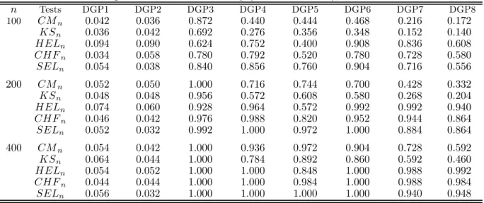
Table 1 reports the empirical rejection frequency of thefive tests, namely,CMn, KSn, HELn, CHFn and SELn, for nominal size 5%. Given the computational burden, we consider three sample sizes:
n = 100, 200 and 400. We use 500 replications for all tests when the null is true and 250 replications when the null is false. We apply 200 bootstrap resamples in each replication. From Table 1, we see that the sizes of allfive tests are reasonably well-behaved, despite the fact that theHELn test is moderately oversized for small sample sizes. In terms of power, we observe that the three kernel-based testsHELn,
CHFn andSELn tend to be more powerful thanLG’s testsCMn and KSn. Interestingly,HELn has the largest power in detecting alternatives in DGPs 7-8. SELn outperforms the other tests in terms of power in DGPs 3-6 but is slightly outperformed byCHFn andHELn in DGPs 7-8.
Table 1: Comparison of tests for causality (d1=d2=d3= 1), nominal level: 0.05 n Tests DGP1 DGP2 DGP3 DGP4 DGP5 DGP6 DGP7 DGP8 100 CMn 0.042 0.036 0.872 0.440 0.444 0.468 0.216 0.172 KSn 0.036 0.042 0.692 0.276 0.356 0.348 0.152 0.140 HELn 0.094 0.090 0.624 0.752 0.400 0.908 0.836 0.608 CHFn 0.034 0.058 0.780 0.792 0.520 0.780 0.728 0.580 SELn 0.054 0.038 0.840 0.856 0.760 0.904 0.716 0.556 200 CMn 0.052 0.050 1.000 0.716 0.744 0.700 0.428 0.332 KSn 0.048 0.048 0.956 0.572 0.608 0.580 0.268 0.204 HELn 0.074 0.060 0.928 0.964 0.572 0.992 0.992 0.940 CHFn 0.046 0.042 0.976 0.988 0.820 0.952 0.944 0.864 SELn 0.052 0.032 0.992 1.000 0.972 1.000 0.884 0.864 400 CMn 0.054 0.042 1.000 0.936 0.972 0.904 0.728 0.592 KSn 0.064 0.044 1.000 0.784 0.892 0.860 0.592 0.460 HELn 0.054 0.052 1.000 1.000 0.848 1.000 0.988 0.992 CHFn 0.044 0.044 1.000 1.000 0.984 1.000 0.988 0.984 SELn 0.056 0.032 1.000 1.000 1.000 1.000 0.940 0.948
DGP10: Wt= (ε01,t, ε2,t, ε3,t)0,where both{ε1,t}and{ε2,t, ε3,t}are IIDN(0, I2).
For DGP20 through DGP80,W t= ((Yt−1, Yt−2), Yt, Zt−1)0, DGP20: Yt= 0.5Yt−1+ 0.25Yt−2+ε1,t; DGP30: Yt= 0.5Yt −1+ 0.25Yt−2+ 0.5Zt−1+ε1,t; DGP40: Y t= 0.5Yt−1+ 0.25Yt−2+αZt2−1+ε1,t; DGP50: Yt=αYt −1Zt−1+ 0.25Yt−2+ε1,t; DGP60: Y t= 0.5Yt−1+ 0.25Yt−2+ 0.55Zt−1ε1,t; DGP70: Yt=√htε1,t, ht= 0.01 + 0.5Yt2−1+ 0.25Yt2−2+ 0.25Zt2−1; DGP80: same as DGP8;
whereZt= 0.5Zt−1+ε2,tand{ε1,t, ε2,t}is IIDN(0, I2)in DGPs 20-70.
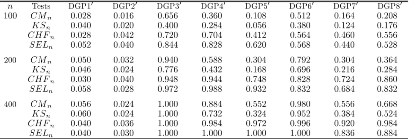
In view of the difficulty in implementing the HELn test because of bandwidth selection, we only study thefinite sample behavior of the other four tests. We use the same kernels, weighting functions, number of replications, and number of bootstrap resamples as before. The bandwidth selection rule for theCHFn andSELn tests is also the same as in case 1.
Table 2 reports the empirical size and power properties of the four tests. As in thefirst case, the sizes are reasonably well behaved for all tests and theSELn andCHFn tests tend to dominate theLGtests in terms of power. TheCHFntest dominatesCMnandKSnfor all nonlinear DGPs under investigation,
SELn exhibits significantly greater empirical power than CHFn in DGPs 30-60, but it is the other way around in DGPs 70-80. As expected, in comparison with DGP8, DGP80 suggests that the power of our tests would be adversely affected as the dimension of the conditioning variable increases.
For the third case(d1= 3, d2=d3= 1), we use the following DGPs:
DGP100: Wt= (ε1,t, ε2,t, ε3,t)0,where {ε1,t}is IIDN(0, I3)and {ε2,t, ε3,t}is IIDN(0, I2).
For DGP200 through DGP700,W
t= ((Yt−1, Yt−2, Yt−3), Yt, Zt−1)0,
DGP200: Yt= 0.5Yt−1+ 0.25Yt−2+ 0.125Yt−3+ε1,t;
DGP300: Yt= 0.5Yt
Table 2: Comparison of tests for causality (d1= 2, d2=d3= 1), nominal level: 0.05 n Tests DGP10 DGP20 DGP30 DGP40 DGP50 DGP60 DGP70 DGP80 100 CMn 0.028 0.016 0.656 0.360 0.108 0.512 0.164 0.208 KSn 0.040 0.020 0.400 0.284 0.056 0.380 0.124 0.176 CHFn 0.028 0.042 0.720 0.704 0.412 0.564 0.460 0.556 SELn 0.052 0.040 0.844 0.828 0.620 0.568 0.440 0.528 200 CMn 0.050 0.032 0.940 0.588 0.304 0.792 0.304 0.364 KSn 0.046 0.024 0.776 0.432 0.168 0.696 0.216 0.284 CHFn 0.030 0.040 0.948 0.944 0.748 0.828 0.724 0.860 SELn 0.058 0.028 0.972 0.988 0.932 0.832 0.684 0.832 400 CMn 0.056 0.024 1.000 0.884 0.552 0.980 0.556 0.668 KSn 0.060 0.024 1.000 0.732 0.324 0.952 0.384 0.524 CHFn 0.040 0.036 1.000 0.984 0.972 0.996 0.920 0.984 SELn 0.040 0.030 1.000 1.000 1.000 1.000 0.836 0.884 DGP400: Yt= 0.5Yt −1+ 0.25Yt−2+ 0.125Yt−3+ 0.5Zt2−1+ε1,t; DGP500: Y t= 0.5Yt−1Zt−1+ 0.25Yt−2+ 0.125Yt−3+ε1,t; DGP600: Yt= 0.5Yt −1+ 0.25Yt−2+ 0.125Yt−3+ 0.55Zt−1ε1,t; DGP700: Y t=√htε1,t, ht= 0.01 + 0.5Yt2−1+ 0.25Yt2−2+ 0.125Yt2−3+ 0.5Zt2−1; DGP800: same as DGP8;
whereZt= 0.5Zt−1+ε2,t, and{ε1,t, ε2,t}is IIDN(0, I2)in DGPs 200-700.
We use the same kernels, weighting functions, number of replications, and number of bootstrap resamples as in the first case. The main difference is that we need to adjust the LSCV bandwidths slightly to meet the conditions in Assumption A2(iii). We first set h1 = c1n−1/(4+d1+d3) and h2 =
c2n−1/(8+d1) and choose c1 and c2 by using the LSCV. Then we adjust h1 to be h∗1n1/(4+d1+d3)n−1/8.5
where h∗
1 is the LSCV bandwidth for h1. Consequently, the resulting bandwidths satisfy h1 ∝ n−1/8.5
andh2∝n−1/(8+d1).In view ofd1+d3= 4, n= 100is too small for any nonparametric test to be well
behaved. Thus, we only consider n = 200 and 400 in Table 3. Table 3 reports the empirical size and power behavior of our tests. Apparently, the results are similar to the second case above.
Table 3: Comparison of tests for causality (d1= 3, d2=d3= 1), nominal level: 0.05
n Tests DGP100 DGP200 DGP300 DGP400 DGP500 DGP600 DGP700 DGP800 200 CMn 0.050 0.028 0.756 0.484 0.192 0.788 0.260 0.448 KSn 0.048 0.032 0.500 0.380 0.096 0.660 0.212 0.372 CHFn 0.028 0.022 0.964 0.952 0.668 0.852 0.552 0.856 SELn 0.056 0.026 0.996 0.980 0.860 0.816 0.344 0.680 400 CMn 0.050 0.032 0.992 0.728 0.400 0.912 0.390 0.620 KSn 0.044 0.036 0.840 0.552 0.220 0.880 0.306 0.568 CHFn 0.032 0.034 1.000 0.972 0.928 0.884 0.792 0.972 SELn 0.056 0.038 1.000 1.000 1.000 0.888 0.616 0.876
6
Applications to macroeconomic and
fi
nancial time series
Although many studies conducted during the 1980s and 1990s report that economic and financial time series, such as exchange rates and stock prices, exhibit nonlinear dependence (e.g., Hsieh 1989, 1991; Sheedy, 1998), researchers often neglect this when they test for Granger causal relationships. In this section, wefirst study the dynamic linkage between pairwise daily exchange rates across some industri-alized countries by using both our SELR test (T˜n1) for CI and the traditional linear Granger causality
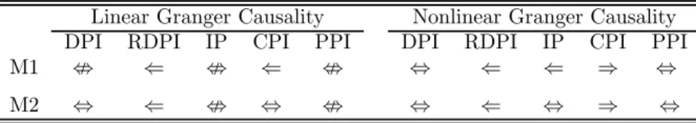
test. Then with the same techniques, we study the dynamic linkage between three US stock market price indices and their trading volumes. Finally, we investigate the relationship between money supply, output, and prices for the U.S. economy.
6.1
Application 1: exchange rates
Over the last two decades much research has focused on the nonlinear dependence exhibited by foreign exchange rates, but few studies have examined nonlinear Granger causal links between intra-market exchange rates. One exception is Hong (2001) who proposes a test for volatility spillover and applies it to study the volatility spillover between two weekly nominal U.S. dollar exchange rates, the Deutschemark and the Japanese Yen. He finds a change in past Deutschemark volatility Granger-causes a change in current Japanese Yen volatility but a change in past Japanese Yen volatility does not Granger-cause a change in current Deutschemark volatility.
In this application, we apply our nonparametric test to data for the daily exchange rates for three industrialized countries (Canada, Japan, and the UK) and the European Union (EU), and compare the results to those using a conventional linear test for Granger causality. The data are from Datastream, with the sample period running from January 2nd, 2002 to April 5th, 2011, a total of 2415 observations. The exchange rates are the local currency against the US dollar. Nevertheless, due to national holidays or certain other reasons, some observations for exchange rates are missing. Also, different nations have different national holidays and thus different missing observations. Because we do causality tests with exchange rates from countries pairwise , if the observation for one country is missing, we also delete that for the other country of the pair. Following the literature, we letEtstand for the natural logarithm of exchange rates multiplied by 100. Since both the linear Granger causality test and our nonparametric test require that the time series be stationary and we are interested in the relation between the changes in the exchange rates, we first employ the augmented Dickey-Fuller test to check for stationarity for all four exchange rates. The test results indicate that there is a unit root in all level seriesEt but not in the first differenced series ∆Et. Therefore, both Granger causality tests will be conducted on thefirst differenced data.
Let DX be thefirst differenced exchange rate in Country X and DY thefirst differenced exchange rate in CountryY.The time series{DXt}does not linearly Granger cause the time series{DYt}if the null hypothesisH0,L:β1=· · ·=βLx = 0holds in
DYt=α0+α1DYt−1+· · ·+αLyDYt−Ly+β1DXt−1+· · ·+βLxDXt−Lx+ t, (6.1)
where tis a white noise underH0,L.AnF-statistic can be constructed to check whether the nullH0,Lis true or not. Nevertheless, in order to make a direct comparison with our nonparametric test for nonlinear
Granger causality in the next subsection, we focus on testingH∗0,L:β = 0in
DYt=α0+α1DYt−1+· · ·+αLyDYt−Ly+βDXt−i+ t, i= 1, ..., Lx. (6.2)
Apparently,H∗0,Lis nested inH0,N L.The rejection ofH∗0,N Lindicates the rejection ofH0,N Lbut not the other way around.
To implement our test, we set all parameters according to those used in our simulations. The null of interest is now H0,N L: Pr £ F(DYt|DYt−1, ..., DYt−Ly;DXt−1, ..., DXt−Lx) =F(DYt|DYt−1, ..., DYt−Ly) ¤ = 1. (6.3) Due to the “curse of dimensionality,” we allow onlyLy=1, 2, or 3. Further, for each test we only include one laggedDXtin the conditioning set. Thus, we actually test a variant ofH0,N L:
H∗0,N L: Pr £ F(DYt|DYt−1, ..., DYt−Ly;DXt−i,) =F(DYt|DYt−1, ..., DYt−Ly) ¤ = 1, i= 1, ..., Lx. (6.4) Again, H∗
0,N L is nested in H0,N L. The rejection of H∗0,N L indicates the rejection of H0,N L but not the other way around. In this sense, our test is conservative.
For both tests, whenLy is 1, we also chooseLxto be 1 so that we only check whetherDXt−1 should
enter (6.2) or (6.4) or not. WhenLyis 2, we chooseLxto be 2. In this case, we check whetherDXt−1or
DXt−2(but not both) should enter (6.2) or (6.4) or not. The case forLy= 3is analogous. Consequently, for each test, we have six possible results. If any of these results suggest that we should reject the null at the 1% nominal level,8 then we indicate that there is linear or nonlinear Granger causality fromDX toDY.
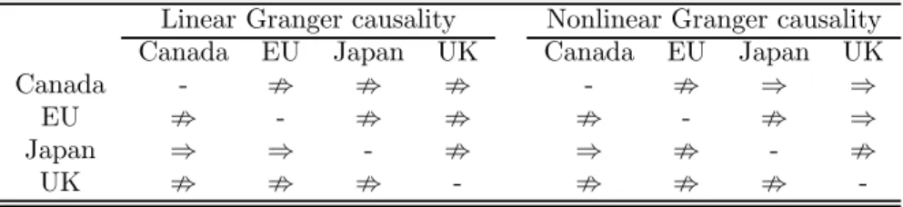
Table 4: Bivariate linear Granger causality test between exchange rates (nominal level: 1%) Linear Granger causality Nonlinear Granger causality
Canada EU Japan UK Canada EU Japan UK
Canada - ; ; ; - ; ⇒ ⇒
EU ; - ; ; ; - ; ⇒
Japan ⇒ ⇒ - ; ⇒ ; - ;
UK ; ; ; - ; ; ;
-We summarize the results in Table 4, where ⇒and;signify the presence and absence of Granger-causality from the column variable to the row variable, respectively, and the nonlinear tests are based on the bootstrapp-values obtained from 400 bootstrap resamples. First, the linear Granger test reveals only two unidirectional Granger causal links among the four exchange rate series: the exchange rate for Japan Granger-causes that for Canada and EU. Second, our nonparametric test fails to detect the linear Granger-causality from Japan’s exchange rate to the EU’s but can reveal another three more causal links among the four exchange rate series, some of which are bidirectional (Canada ⇔Japan). One obvious reason for the failure of the linear Granger causality test to detect any bidirectional causal linkages is
8This gives the Bonferroni bound 6%, comparable with the widely used nominal significance level 5%. Such a multiple procedure also applies to Applications 2 and 3 below.
that exchange rates exhibit unambiguously nonlinear dependence across markets. The volatility spillover between exchange rates (see Hong (2001) and the reference there) is a special case of such nonlinear dependence. Third and interestingly, neither test suggests a Granger-causal relationship between the exchanges rates of Canada or Japan and the EU.
6.2
Application 2: stock price and trading volume
There are several explanations for the presence of a bidirectional Granger causal relation between stock prices and trading volume. For brevity, we only mention two of them. The first one is the sequential information arrival model (e.g., Copeland, 1976) in which new information flows into the market and is disseminated to investors one at a time. This pattern of information arrival produces a sequence of momentary equilibria consisting of various stock price-volume combinations before a final, complete information equilibrium is achieved. Due to the sequential informationflow, lagged trading volume could have predictive power for current absolute stock returns and lagged absolute stock returns could have predictive power for current trading volume. The other is the noise trader model (e.g., DeLong, 1990) that reconciles the difference between the short- and long-run autocorrelation properties of aggregate stock returns. Aggregate stock returns are positively autocorrelated in the short run, but negatively autocorrelated in the long run. Since noise traders do not trade on the basis of economic fundamentals, they impart a transitory mispricing component to stock prices in the short run. The temporary component disappears in the long run, producing mean reversion in stock returns. A positive causal relation from volume to stock returns is consistent with the assumption made in these models that the trading strategies pursued by noise traders cause stock prices to move. A positive predictive relation from stock returns to volume is consistent with the positive-feedback trading strategies of noise traders, for which the decision to trade is conditioned on past stock price movements.
Gallant et al. (1992) argue that more can be learned about the stock market by studying the joint dynamics of stock prices and trading volume than by focusing on the univariate dynamics of stock returns. Using daily data for the Dow Jones price index for the periods 1915-1990, Hiemstra and Jones (1994) study the dynamic relation between stock prices and trading volume and find significant bidirectional nonlinear predictability between them. Here we reinvestigate this issue using the latest daily data for the three major U.S. stock market price indices, i.e., the Dow Jones, the Nasdaq, and the S&P 500, and their associated trading volumes in the NYSE, Nasdaq and NYSE markets, respectively. The data are obtained from Yahoo Finance with the sample period running from January 2nd, 2002 to January 4th, 2011. Following the literature, we let Pt and Vt stand for the natural logarithm of stock price index and volume multiplied by 100, respectively. Both Granger causality tests will be conducted on thefirst differenced data∆Ptand ∆Vt.
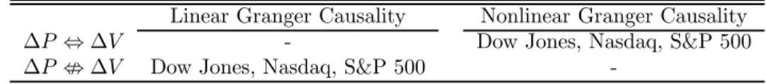
The implementation of both tests is similar to the previous application. As for the case of exchange rates, we conduct both tests for the three major market indices and summarize the results in Table 5, where ⇔signifies the presence of bidirectional Granger causality and< its absence in both directions, and the nonlinear tests are based on the bootstrapp-values obtained from 400 bootstrap resamples. First, the linear Granger causality test suggests there is no Granger causal link between trading volumes and stock prices for all three datasets. Second, our nonparametric test reveals bidirectional Granger causal