Aggregation-cokriging for highly multivariate spatial data

(1)

Zurich Open Repository and Archive University of Zurich Main Library Strickhofstrasse 39 CH-8057 Zurich www.zora.uzh.ch Year: 2011

Aggregation-cokriging for highly multivariate spatial data Furrer, R ; Genton, M G

Abstract: Best linear unbiased prediction of spatially correlated multivariate random processes, often called cokriging in geostatistics, requires the solution of a large linear system based on the covariance and cross-covariance matrix of the observations. For many problems of practical interest, it is impossible to solve the linear system with direct methods. We propose an eﬀicient linear unbiased predictor based on a linear aggregation of the covariables. The primary variable together with this single meta-covariable is used to perform cokriging. We discuss the optimality of the approach under different covariance structures, and use it to create reanalysis type high-resolution historical temperature fields.

DOI: https://doi.org/10.1093/biomet/asr029

Posted at the Zurich Open Repository and Archive, University of Zurich ZORA URL: https://doi.org/10.5167/uzh-58201

Journal Article Published Version Originally published at:

Furrer, R; Genton, M G (2011). Aggregation-cokriging for highly multivariate spatial data. Biometrika, 98(3):615-631.

(2)

C

2011 Biometrika Trust Printed in Great Britain

Aggregation-cokriging for highly multivariate spatial data

BYREINHARD FURRER

Institute of Mathematics, University of Zurich, 8057 Zurich, Switzerland [email protected]

ANDMARC G. GENTON

Department of Statistics, Texas A&M University, College Station, Texas 77843, U.S.A. [email protected]

SUMMARY

Best linear unbiased prediction of spatially correlated multivariate random processes, often called cokriging in geostatistics, requires the solution of a large linear system based on the covari-ance and cross-covaricovari-ance matrix of the observations. For many problems of practical interest, it is impossible to solve the linear system with direct methods. We propose an efficient linear unbi-ased predictor bunbi-ased on a linear aggregation of the covariables. The primary variable together with this single meta-covariable is used to perform cokriging. We discuss the optimality of the approach under different covariance structures, and use it to create reanalysis type high-resolution historical temperature fields.

Some key words: Climate; Cokriging; Eigendecomposition; Intrinsic process; Linear unbiased prediction.

1. INTRODUCTION

The prediction of a geophysical quantity based on observations at nearby locations of the same quantity and on other related variables, so-called covariables, is often of interest. Typical examples are drawing pollution maps, establishing flood plans or simply predicting temperatures. Obviously, all available observations should be taken into account, and their contributions ought to be weighted by the strength of their correlation with the location of interest. In many of those applications, we have large or even massive amounts of data available, implying the need for a careful choice of methodology in order to keep the analysis computationally feasible.

For a single variable of interest, spatial best linear unbiased prediction, i.e., kriging, has been intensively studied and many approaches exist; seeSun et al.(2011) for a recent review. However, if information from several different variables is available, this information should be used for prediction and a classical approach is cokriging. Unfortunately, the problems implied by large amounts of data are then further amplified.

We assume that we have a primary variable and two or more secondary variables. We aim at predicting the primary variable at some location based on observations of the primary variable at a set of distinct locations and on observations of the secondary variables at a possibly different set of distinct locations, i.e. a particular form of cokriging.

Cokriging was extensively studied in the late 1980s and early 1990s (e.g.,Davis & Greenes, 1983;Abourfirassi & Marino,1984;Carr & McCallister,1985). For a more theoretical discus-sion see, for example, Myers(1982, 1992), Ver Hoef & Cressie (1993, 1994) and references

at Zentralbibliothek on February 6, 2012

http://biomet.oxfordjournals.org/

(3)

therein. However, since the cokriging system is of orderO(N2), where N is the total number of observations, practitioners often try to reduce the number of equations by taking into account only a few neighbours of the prediction location.Myers(1983) andLong & Myers (1997) provided other solutions to reduce the computational burden of cokriging, based on linear combinations or linear approximations. Another common tool is coregionalization (e.g.,Journel & Huijbregts, 1978;Gelfand et al.,2004). Each component of the process is assumed to be a linear combina-tion of orthogonal random funccombina-tions. The orthogonality is exploited with a linear transforma-tion, reducing the multivariate setting to a univariate one. However, the transformation has to be estimated, often iteratively, cancelling out the computational gains (e.g.,Bourgault & Marcotte, 1991). Finally, the extremely simple alternative solution of full cokriging in a moving neighbour-hood is often used in practice, see, for example, Haas (1990a,1990b). The moving neighbourhood approach is quite useful when predicting at a limited number of locations (e.g.,Johns et al.,2003) but has disadvantages, such as the potential introduction of discontinuities.

For the applications of interest to us, in numerical weather prediction, the linear systems involved in calculating the best linear unbiased predictor and its mean squared prediction error are often too large to use direct methods. We present a novel approach to reduce this computa-tional burden, by aggregating the secondary variables with carefully chosen weights. The result-ing combination of secondary variables should contribute as much as possible to the prediction of the primary variable in the mean squared prediction error sense. The prediction is then performed using a cokriging approach with the primary variable and the aggregated secondary variables. This reduces the computational burden of the prediction from solving a(n+ℓm)×(n+ℓm)to solving a(n+m)×(n+m)linear system, wherenandmare the numbers of observations of the primary and secondary variables, respectively, andℓis the number of secondary variables. We assumenandm to be such that we are able to solve a(n+m)×(n+m)linear system but not a(n+ℓm)×(n+ℓm)one. By construction we know that the resulting mean squared pre-diction error lies between that of kriging and of cokriging. Since the computational complexity is comparable with bikriging, i.e. cokriging with only one of the secondary variables, we aim for a mean squared prediction error between bikriging and cokriging.

2. AGGREGATION-COKRIGING

2·1. Definitions and basic properties

We assume that we have a primary variable, denoted by Y0(·), and two or more secondary variables, denoted by Y1(·), . . . ,Yℓ(·),ℓ >1. We aim to predict the primary variable at a new locationsp based on observations and we writeY0(sp)=Yp, where the subscript p stands for

predict. We assumen observations from distinct locations of the primary variable, denoted by Y0, as well asmobservations from distinct locations of each of the secondary variables, denoted by Y1, . . . ,Yℓ. We use a generic notation for the indices of the secondary variable(s), e.g.,Yg

might be the vectorY1, or(Y₁T, . . . ,YℓT)T, or a linear combination thereof. Accordingly, the ele-ments of var(Yg)=gg are determined by the covariance structure of the secondary variables

cov(Yi,Yj)=i j (i,j=1, . . . , ℓ). Further, we assume that the first moment of the multivariate

random process is zero and for the second moment we write

var ⎛ ⎝ Yp Y0 Yg ⎞ ⎠= ⎛ ⎝ pp p0 pg 0p 00 0g gp g0 gg ⎞ ⎠, (1)

wherepp=var(Yp),00=var(Y0),p0=cov(Yp,Y0), etc. By separating between prediction Yp and primary variable Y0, we can incorporate measurement errors. For example, denote a

(4)

Aggregation-cokriging

covariance function by c(si,sj), then pp=c(sp,sp) and [00]i j=c(si,sj)+τ2I(si =sj)

withτ2the magnitude of the measurement error andI the indicator function. The best linear unbiased predictor ofYpgivenY0andYgis

p0pg 00 0g g0 gg −1 Y0 Yg , (2)

and its mean squared prediction error is given by

pp−p0pg 00 0g g0 gg −1 0p gp . (3)

We now introduce the aggregation-cokriging method. For each location si (i=1, . . . ,m),

where the secondary variable is observed, we need to find an ℓ-vector a(si)=

{a1(si), . . . ,aℓ(si)}Twhich defines the weights forY1(si), . . . ,Yℓ(si). To simplify the exposition,

we define the aggregation matrixA∈Rm×mℓ, such that the corresponding linear combination of the secondary variables is simply AY, withY=(YT

1, . . . ,YℓT)T. Then, in (1)–(3),Yg isAY,

and the corresponding covariance matrices are calculated accordingly, e.g.,gg=Avar(Y)AT.

The matrixggis positive definite and the inverse in (2) exists ifAhas full row rank.

The aggregation matrix takes the form A= {diag(L₁), . . . ,diag(Lℓ)}, with Lr= {ar(s1), . . . ,ar(sm)}T. The ith row of A is a(si)T⊗eT_i where ⊗ is the Kronecker product

andei is theith canonical basis vector. In the special case where the weights do not change with

the location si, A=(a1I, . . . ,aℓI)=aT⊗I, where I ∈Rm×m is the identity matrix. In this notation, bikriging with the first variable corresponds toA=(I,0, . . . ,0)=eT

1⊗I.

To relate or link the aggregation scheme to the resulting mean squared prediction error, let E−1=A(Y Y−Y0−₀₀10Y)AT, whereY Yis the covariance matrix ofYandY0=T₀Y

is the cross-covariance matrix betweenY andY0, and define the function

g(A)=

A(Yp−Y000−10p)2E ifE is positive definite,

0 otherwise,

where z2_E=zT_{E z} _and

Yp is the cross-covariance matrix between Y and Yp. The mean

squared prediction error based on the aggregation matrixAis

MSPE(A)=pp−p0−₀₀10p−g(A), (4)

and minimizing (4) over all admissibleAis equivalent to maximizingg(A). IfA=aT_⊗_I_{, we} abbreviate tog(a). For example, g(0)=0 andg(er)are linked to the mean squared prediction

error of simple kriging and bikriging with therth variable, respectively.

Direct maximization of g(A)overA is only possible in very specific cases, and numerical maximization often requires more computational effort than solving the best linear unbiased pre-dictor with all secondary variables. We now propose a few aggregation schemes that are intuitive and suboptimal. We choose the weight vectors as the solution of

a(si)=argmax x xT_A ix −λ(xTBix −1), (5) a(si)=argmin x xTCix−λ(xTω−1), (6) at Zentralbibliothek on February 6, 2012 http://biomet.oxfordjournals.org/ Downloaded from

(5)

where Ai ∈Rℓ×ℓis symmetric positive semidefinite,Bi,Ci∈Rℓ×ℓare symmetric positive

def-inite,ω∈Rℓhas at least one nonzero element andλis the Lagrange multiplier. Cokriging with the aggregation matrix A based on (5) and on (6) will be called AGG(A_i,B_i)-cokriging and AGG(Ci, ω)-cokriging, respectively. It is straightforward to show that the solution of (5) isa(si)=

B_i−1/2αi, whereαi is the eigenvector associated with the largest eigenvalue of B_i−1/2AiB_i−1/2

and the solution of (6) isa(si)=C_i−1ω/(ωTC_i−1ω). If the aggregation matrixAis based on the

vectorsa(si)(i=1, . . . ,m), we also writeAGG{a(s_i)a(s_i)T,I}-cokriging.

Individually rescaling the weight vectors a(si) (i=1, . . . ,m) has no effect. Hence, we

will often scale the weight vectors to a(si){a(si)Ta(si)}−1/2 or a(si){a(si)T1}−1, provided

a(si)T1=| 0, to simplify theoretical concepts.

LEMMA1. Prediction and mean squared prediction error of aggregation-cokriging based on

the weight vectors a(si)are independent of any scalingγia(si), withγi=| 0 (i=1, . . . ,m).

For cleverly chosen Ai and Bi, orCi andω, the weight vectors obtained with this approach

are not too far from the exact optimum under certain covariance models.

2·2. Example: canonical correlation analysis

An intuitive choice of the weight vectora(si)= {a1(si), . . . ,aℓ(si)}Tis such that the

correla-tion corr{Yp,a1(si)Y1(si)+ · · · +aℓ(si)Yℓ(si)}is maximized. The solution of this optimization

is a particular case of canonical correlation analysis, see, e.g.,Mardia et al.(1979).

PROPOSITION1. Assume that cov{Y_p,Y_r(s_i)} |=0 for at least one r . The vector a(s_i)= {a1(si), . . . ,aℓ(si)}Tmaximizingcorr{Yp,a1(si)Y1(si)+ · · · +aℓ(si)Yℓ(si)}is a(si)=argmaxx

xT_C

i pCpix−λ(xTCiix−1) where the matrices Cii∈Rℓ×ℓ and the vectors Ci p∈Rℓ

(i=1, . . . ,m)are defined by

[Cii]r s=cov{Yr(si),Ys(si)} =[r s]ii (r,s=1, . . . , ℓ), (7)

[Ci p]r=[Cpi]Tr=cov{Yr(si),Yp} =[r p]i (r=1, . . . , ℓ). (8)

The vectora=a(si)depends on the locationssi where the secondary variables are observed

and on the prediction locationsp. Hence, withAGG(C_{i p}C_pi,C_ii)-cokriging, the weightsa(s_i)∈

Rℓ (i=1, . . . ,m) formℓfields, denoted byLr (r=1, . . . , ℓ). For simplicity, we use the term

weights for theseℓfields. By construction, these weights take into account the cross-covariance structure of the secondary variables at the locationssi (i=1, . . . ,m) and they do not take into

account the covariance structure [rr]i j (i=| j) of the individual variables. This means that only

diagonal elements of the cross-covariance matrices enter the calculation of the weight vector a(si), e.g. (7). This fact may lead to rapidly varying weights.

Further, with compactly supported covariance functions (see, e.g.Gneiting,2002) the cross-covariance cov{Y(si),Yp}might be zero, resulting in a zero vectorCi p. In this case, the matrix

C_ii−1/2Ci pCpiC_ii−1/2 has only zero eigenvalues and the question arises what weight vectora(si)

we should choose. Intuitive choices are: therth canonical basis vector, wherer corresponds to the variable also used for bikriging; andℓ−1/21, i.e., all variables receive the same weight. Later we will see that the second case can be competitive but often inferior to the first case, for which we need to determine the variabler, implying additional computational costs.

(6)

2·3. Example: maximum covariance analysis

The canonical correlation based approach has the disadvantage that we need to calculatem vectorsa(si)(i=1, . . . ,m). Instead of simplistically choosing an arbitrary locationsj and using

a(si)=a(sj)for alli, we now discuss a more intuitive procedure for which the weights do not

depend on the locationsi. We propose to maximize the ordinaryL2-norm of

cov Yp, ℓ r=1 arYr = ℓ r=1 arpr, (9) which is tr ⎛ ⎝ ℓ r,s=1 arasr pps ⎞ ⎠= ℓ r,s=1 arastr(r pps)=aT[psr p]a,

under the constraintaT_a₌_{1. Straightforward algebraic manipulations imply that}_a_{is the} eigen-vector associated with the largest eigenvalue of the matrix with elements [psr p]r s. Hence,

we perform AGG(_ps_{r p},I)-cokriging, where I ∈Rℓ×ℓ. This approach is a particular case of

maximum covariance analysis, see, e.g.,Jolliffe(2002).

We could also define the weight vectorsa(si)of§2·2via a covariance instead of a correlation

approach. Or we could constrain the vectora of this section toaT_Ba₌_{1, for some symmetric} positive definite matrix B. These cases would result inAGG(Ci pCpi,I)- andAGG(psr p,

B)-cokriging.

2·4. Generalized intrinsic model for the secondary variables

If we consider constant weights induced bya=(a1, . . . ,aℓ)T, theng(a)takes the form

g(a)= _ℓ r=1 arcr T _ℓ r,s=1 arasSr s −1 _ℓ r=1 arcr , (10)

withcr=r p−r0−0010p andSr s=r s−r0−0010s. Although the previous expression

has well-known derivatives with respect toai, it is only possible in very specific cases to

analyt-ically find the maximum ofg(a). One example of such a simple model is based on the following specification of the covariance matrix:

var ⎛ ⎝ Yp Y0 Y ⎞ ⎠= ⎛ ⎝ pp p0 ωT⊗pc 0p 00 ωT⊗0c ω⊗cp ω⊗c0 ⊗cc ⎞ ⎠, (11)

with ∈Rℓ×ℓa symmetric positive definite matrix andω∈Rℓa vector with at least one nonzero element. The matrixcc∈Rm×mis the common correlation structure of the secondary variables.

Further, up to a constant, pc∈R1×m is the cross-covariance betweenYp and any secondary

variable and0c∈Rn×mis the cross-covariance between the primary variable and any secondary

variable. Without explicitly stating all conditions, we assume that the matrix (11) is positive definite.

Model (11) is more general than the standard intrinsic correlation model, e.g.,Wackernagel (2006, p. 154). In (11), only the secondary variables form an intrinsic correlation model.

(7)

PROPOSITION2. Under the model specified by (11), AGG( , ω)-cokriging minimizes the

mean squared prediction error(3).

In practice, we often have var(Y)=| ⊗cc as, for example, the secondary variables may

have different correlation ranges. A simple approximation of the variance in (11) is illustrated in §4. In the case of stationarity, we could use as a first-order approximation [ r s]=[r s]ii and

ω=[r0]i, for somei. A more formal approximation approach is to find the closest intrinsic

approximation to the covariance structure (1), in a similar spirit toGenton(2007).

2·5. Identical cross-covariance structure

We work through a simple case, assuming that all the secondary variables have the same cross-covariance structure withYp and with the observations of the primary variable.

LEMMA2. Assume that _{r p}=₁_p and_r₀=₁₀ (r=2, . . . , ℓ). Let AandB be

aggre-gation matrices based on aggreaggre-gation vectors a(si)and b(si)with a(si)T1=| 0and b(si)T1=| 0

(i=1, . . . ,m). Then,MSPE(A) <MSPE(B)if and only if the matrix

ℓ r=1 ℓ s=1 r s◦(Hr s−Gr s) (12)

is positive definite, where ◦ is the Schur or direct product, Hr s= {br(s1), . . . ,br(sm)}T

{bs(s1), . . . ,bs(sm)}and Gr s= {ar(s1), . . . ,ar(sm)}T{as(s1), . . . ,as(sm)}.

The proof, given in the Appendix, is based on the fact thatr0−0010s is independent ofr and

s, due to the identical covariance structure. The condition based on (12) is often not practical, but Hr s−Gr s being positive semidefinite for allr andsalso implies positive definiteness of (12)

(Horn & Johnson,1994, Theorem 5·2·1). Further, (12) can be simplified considerably if the sec-ondary variables all have the same cross-covariancer s=12(r=| s=1, . . . , ℓ).

In the case of constant weights,Gr s andHr s are proportional to 11T.

LEMMA3. Assume that_{r p}=₁_pand_r₀=₁₀ (r=2, . . . , ℓ). If the aggregation

matri-cesAandBare based on constant weights given by a and b, thenMSPE(A) <MSPE(B):

(i) if and only ifℓ_r₌₁ℓ_s₌₁r s◦11T{brbs(bT1)−2−aras(aT1)−2}is positive definite;or

(ii) if brbs(aT1)2aras(bT1)2 for all r,s=1, . . . , ℓ, with strict inequality for at least

one pair.

Additionally, ifr s=12(r=| s=1, . . . , ℓ), thenMSPE(A) <MSPE(B)if and only ifℓ_r₌₁K_r ◦

11T_{_b2

r(bT1)−2−ar2(aT1)−2}with Kr=rr−12, is positive definite. Lastly, ifrr=11and

r s=12 (r=| s=1, . . . , ℓ), thenMSPE(A) <MSPE(B)if and only if the weight vectors satisfy

bT_b(bT₁₎−2_>_aT_a(aT₁₎−2_.

COROLLARY1. Assume that _{r p}=₁_p, _r₀=₁₀, _rr=₁₁ and _{r s}=₁₂ (r=| s=

1, . . . , ℓ). If we use the first variable for bikriging, then: (i) if aT₁₌_{0, then g(a)}₌_g(0)₌₀_;

(ii) if|aT₁_{| =}_(aT_a)1/2_{, then g(a)}₌_g(e

1). Further, the equality signs can be replaced with strict inequalities.

Using(4), the statements also relate the mean squared prediction errors.

(8)

PROPOSITION3. Assume thatr p=1p, r0=10, rr=11 and r s=12 (r=| s= 1, . . . , ℓ). The vector a defined in Proposition1 and the vector a ofAGG( , ω)-cokriging are

proportional to1and the mean squared prediction errors of aggregation-cokriging and cokriging

are identical.

The last statement supports using 1 as the weight vector wheneverCi p=0 as discussed in§2·2.

If the secondary variables do not have a common cross-covariance structure, then we cannot derive theoretical results about the performance of aggregation-cokriging. Simulations indicate, however, that aggregation-cokriging is often still very competitive.

2·6. Computational complexity

In order to compare the computational complexity of the methods discussed above, we assume that dot and matrix products and the calculation of inverses are performed in O(n), O(n2) and O(n3) computing time, respectively, although we acknowledge the existence of iterative methods which are of lower order, e.g., Billings et al. (2002). Calculating an inverse −1 can often be avoided by solving the associated linear system instead, which is usually done with a Cholesky decomposition of , generally of order O(n3) and two triangular solves, generally of order O(n2). Assume that we know the covariance structure and its parameters. Then for prediction with zero mean, we need to solve a linear system, perform a matrix-vector and a vector-vector multiplication, see (2). For kriging, bikriging and cokriging, the associated size is n, n+m andn+ℓm, respectively. Aggregation-cokriging is on top of calculating the weight vectors, as complex as bikriging. Calculating the weight vectors forAGG(C_{i p}C_pi,C_ii)-cokriging

andAGG(_ps_{r p},I)-cokriging is of order O(mℓ3)andO(ℓ3+ℓm), negligible compared with

the prediction step. If the secondary variables are second-order stationary,Cii is independent of

i, and we only need to calculateC_ii−1/2once.

In practice, the first two moments must often be estimated. Assuming that the mean is a linear combination ofk known basis functions besides the vector-vector products, the computational complexity increases from solving one to solvingk+1 linear systems. As the Cholesky decom-position dominates the calculation, the order of complexity of the computation does not change. An unknown second moment structure implies a much heavier computational burden, often requiringO(n2)or evenO(n3)computing time. Hence, another advantage ofAGG(C_{i p}C_pi,C_ii

)-cokriging is that it requires only the cross-covariances cov{Yr(si),Ys(si)}at identical locations

but not the cross-covariances cov{Yr(si),Ys(sj)}(i=| j) of the secondary variables. After the

aggregation,ggis estimated directly from the meta-covariableAY.

3. NUMERICAL COMPARISON

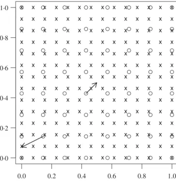
We illustrate variants of the proposed method with simple cases and contrast their mean squared prediction error with bikriging and cokriging. Throughout this section, we assume Gaussian processes with a primary variable observed at n=82 equispaced locations and three secondary variables (ℓ=3) observed atm=142equispaced locations in the unit square [0,1]2. We perform prediction along two paths situated near the edge and at the centre of the domain, see Fig.1. We assume a zero first moment and that the cross-covariances are given by isotropic stationary spherical covariance functions

c(h;θ1, θ2)=θ1max(0,1−h2θ₂−2){1+h(2θ2)−1}, θ1, θ2>0. (13)

(9)

0.0 0.2 0.4 0.6 0.8 1.0 0·0 0·2 0·4 0·6 0·8 1·0

Fig. 1. Layout of the locations for the primary variables (circles) and the secondary variables (crosses). The two arrows indicate the

paths along which we predicted.

Table 1.Parameter values of the spherical covariance matrix for the four different examples

Example 1 2 3 4 Sillθ1 ⎛ ⎜ ⎜ ⎝ 1 0·3 0·25 0·2 1 0·2 0·3 1 0·2 1 ⎞ ⎟ ⎟ ⎠ ⎛ ⎜ ⎜ ⎝ 1 0·3 0·3 0·1 1 0·3 0·2 1 0·3 1 ⎞ ⎟ ⎟ ⎠ ⎛ ⎜ ⎜ ⎝ 1 0·45 0·3 0·1 1 0·3 0·2 1 0·3 1 ⎞ ⎟ ⎟ ⎠ ⎛ ⎜ ⎜ ⎝ 1 0·6 0·1 0·1 1 0·1 0·1 1 0·1 1 ⎞ ⎟ ⎟ ⎠ Rangeθ2 ⎛ ⎜ ⎜ ⎝ 1·2 0·7 0·7 0·7 0·6 0·6 0·6 0·6 0·6 0·6 ⎞ ⎟ ⎟ ⎠ ⎛ ⎜ ⎜ ⎝ 1 0·6 0·5 0·4 0·5 0·3 0·2 0·2 0·1 0·1 ⎞ ⎟ ⎟ ⎠ ⎛ ⎜ ⎜ ⎝ 1 0·6 0·5 0·4 0·5 0·3 0·2 0·2 0·1 0·1 ⎞ ⎟ ⎟ ⎠ ⎛ ⎜ ⎜ ⎝ 1 0·6 0·1 0·1 0·5 0·1 0·1 0·1 0·1 0·1 ⎞ ⎟ ⎟ ⎠

The components match the parameters of the corresponding primary and secondary variables, e.g. the elements [·]12contain the parameters of the cross-covariance between the primary and the first secondary variable.

We callθ1the sill andθ2the range. To simplify the notation, we assume thatYp andY0have the same second moment structure, i.e.,τ2=0. In what follows, we discuss four examples of differ-ent cross-covariance parameter combinations all resulting in positive definite covariance matri-ces. The parameter values of the spherical covariances are given in Table1. Those of Example 1 are chosen so that it represents an intrinsic model (11). Example 2 does not represent a specific covariance structure but the parameters are chosen to ensure positive definiteness. Example 3 is almost identical to Example 2 except for one different sill value, to explore the sensitivity of small changes. The last example is such that there is only considerable correlation between the primary and the first secondary variable. The secondary variables of all examples are ordered such that bikriging with the first and the third variable has the smallest and the largest mean squared prediction error, respectively.

We compare AGG(C_{i p}C_pi,C_ii)-, AGG(C_{i p}C_pi,I)-, AGG(_pr_sp,I)-, AGG( , ω)- and, AGG(11T,I)-cokriging, i.e., aggregation-cokriging based on the vector 1. Only Example 1 is of

(10)

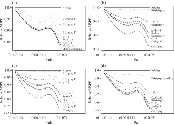
Aggregation-cokriging Path Relative MSPE (0·14,0·14) (0·06,0·11) (0,0·07) 0·85 0·90 0·95 1·00 Kriging BikrigingY3 BikrigingY2 BikrigingY1 11T_,_I Ci pCpi,I ΣprΣsp,I Ci pCpi,Ci i Ω, ω ≅Cokriging (a) Path Relative MSPE (0·14,0·14) (0·06,0·11) (0,0·07) 0·85 0·90 0·95 1·00 Kriging BikrigingY3 11T_,_I BikrigingY2 Ci pCpi,I ΣprΣsp,I BikrigingY1 Ω, ω Ci pCpi,Ci i Cokriging (b) Path Relative MSPE (0·14,0·14) (0·06,0·11) (0,0·07) 0·70 0·75 0·80 0·85 0·90 0·95 1·00 Kriging BikrigingY3 BikrigingY2 11T_,_I Ci pCpi,I ΣprΣsp,I Ω, ω Ci pCpi,Ci i BikrigingY1 Cokriging (c) Path Relative MSPE (0·14,0·14) (0·06,0·11) (0,0·07) 0·5 0·6 0·7 0·8 0·9 1·0 Kriging BikrigingY2andY3 11T_,_I Ci pCpi,Ci i BikrigingY1 ΣprΣsp,I Ci pCpi,I Ω, ω Cokriging (d)

Fig. 2. Relative mean squared prediction error along the path in the lower left corner of Fig.1for the four examples with parameters in Table1. Bikriging and aggregation-cokriging approaches are dotted and dashed, respectively.AGG(A_i,B_i)-cokriging is denoted by ‘A_i,B_i’. The labels are ordered according to the relative mean

squared prediction error at the endpoint.

the form (11) and we approximate the covariance structure of Examples 2 to 4 with an intrinsic structure var(Y)∼ ⊗cc, where contains the respective sills andccis unspecified.

Figure2gives the relative mean squared prediction error along the path in the lower left corner of Fig. 1. The mean squared prediction errors are bounded by the kriging and the cokriging curves. The local minima at (0·06,0·11) are due to the close observation of the secondary variable. Except in Example 3, several aggregation-cokriging schemes outperform bikriging. Among the aggregation-cokriging schemes, AGG(C_{i p}C_pi,C_ii)- andAGG( , ω)-cokriging have in seven out

of eight cases the smallest and second smallest relative mean squared prediction error.

The figure for the relative mean squared prediction error along the path at the centre of Fig.1 is very similar and Table 2 gives the relative mean squared prediction error for its end point (0·5,0·5). Because more primary observations are available at the centre, it is much harder to compete with bikriging with the first variable, which has the lowest relative mean squared pre-diction error in two cases. In three cases, AGG(C_{i p}C_pi,C_ii)-cokriging has the second smallest

relative mean squared prediction error andAGG( , ω)-cokriging has the third smallest relative

mean squared prediction error in Examples 2 to 4.

Although still competitive,AGG(C_{i p}C_pi,I)-cokriging andAGG(_pr_sp,I)-cokriging often

have a slightly higher relative mean squared prediction error than their computationally equiv-alent counterpartsAGG(C_{i p}C_pi,C_ii)-cokriging andAGG( , ω)-cokriging, respectively. Of both

approaches,AGG(_pr_sp,I)-cokriging performs slightly better in general.

Introducing a nugget effect or scaling all ranges does not change the overall picture. The sys-tem is however often sensitive to a change of the sill parameters. As illustrated by Examples 2

(11)

Table 2.Relative mean squared prediction error for the prediction at(0·5,0·5)

Example Bikriging with Aggregation-cokriging with arguments Cokriging

Y1 Y2 Y3 Ci pCpi,Cii Ci pCpi,I prsp,I , ω 11T,I

1 0·961 0·973 0·983 0·941∗∗ 0·942 0·942 0·941∗ 0·944 0·941 2 0·959∗ 0·972 0·993 0·963∗∗ 0·967 0·966 0·965 0·971 0·920 3 0·900∗ 0·972 0·993 0·916∗∗ 0·937 0·933 0·923 0·947 0·809 4 0·775∗∗ 0·987 0·987 0·811 0·798 0·775∗ 0·777 0·925 0·770

∗_{Smallest value among bikriging and aggregation-cokriging.}∗∗_{Second smallest value among value among bikriging}

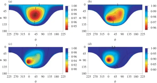
and aggregation-cokriging. ϑ φ 0·95 0·96 0·97 0·98 0·99 1·00 180 135 90 45 0 225 270 315 0 45 90 180 225 (a) ϑ ϑ ϑ φ φ φ 0·96 0·97 0·98 0·99 1·00 180 135 90 45 0 225 270 315 0 45 90 135 180 225 (b) 0·90 0·92 0·94 0·96 0·98 1·00 180 135 90 45 0 225 270 315 0 45 90 135 180 225 (c) 0·80 0·85 0·90 0·95 1·00 180 135 90 45 0 225 270 315 0 45 90 135 180 225 (d) 135 3 3 2,3 3

Fig. 3. Relative mean squared prediction error based on cokriging with an aggregation vectoraT₁_{0 defined by} the spherical angles(ϑ, φ)for prediction at location (0·5,0·5). The contour lines are the relative mean squared pre-diction error for bikriging with the three secondary variablesa=ei(i=1,2,3), and hence passing through the

spherical angles(0,90),(90,90)and(0,0). The numerical minimum is denoted with+. The aggregation vectors forAGG(prsp,I)-,AGG( , ω)- andAGG(11T_,_I₎_{-cokriging are indicated with}_,◦_and_△_{, respectively.}

and 3, a change in the sill of the cross-covariance between the primary and the first secondary variable from 0·3 to 0·45 not only changes the relative mean squared prediction error dramati-cally, but even the corresponding weights.

The examples illustrate that there is unfortunately no general rule to choose the aggrega-tion scheme. We advocate using AGG( , ω)-cokriging, especially if the covariance structure is

close to an intrinsic model (11). Otherwise,AGG(C_{i p}C_pi,C_ii)-cokriging should be favoured or AGG(_pr_sp,I)-cokriging if computation time prohibits the former, in all cases with plug-in

estimates where necessary.

For a low-dimensional setting as given here, we can numerically find the aggregation vector a by directly maximizingg(a), i.e. minimizing the mean squared prediction error. As an illus-tration, we perform a grid search over all vectorsa,aT_a₌_{1, when predicting at (0}_·_5,0_·_{5). We} use spherical coordinates and represent all vectorsaby the anglesϑandφ. Figure3shows rel-ative mean squared prediction error as a function of a foraT₁_{0. The plane}_aT₁₌_{0 divides} the sphere in two half spheres which are symmetric with respect to the mean squared prediction error. This explains the bowl shape of the area in Fig.3. The contour lines give the relative mean

(12)

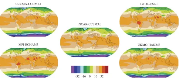
Aggregation-cokriging CCCMA-CGCM3.1 NCAR-CCSM3.0 GFDL-CM2.1 UKMO-HadCM3 MPI-ECHAM5 -32 -16 0 16 32

Fig. 4. September 1957 average temperature model output from five general circulation models in degrees Cel-sius. The data are interpolated to a 5×5 degree latitude-longitude resolution.

squared prediction error for the bikriging approaches with the three secondary variables, corre-sponding toa=ei (i=1,2,3) and the aggregation vectors forAGG(_pr_sp,I)-,AGG( ,

ω)-and AGG(11T,I)-cokriging are indicated as well. In Example 1, AGG( , ω)-cokriging and the

numerically found minimum mean squared prediction error coincides with the aggregation vector (0·754,0·589,0·292)T_{, which is (38}◦_,73◦_{) in spherical coordinates. For Example 4 relatively few} angles lead to a smaller mean squared prediction error compared with bikriging with the first variable, in other words, the contour encloses a very small area.

4. IMPUTATION OF OBSERVED TEMPERATURE FIELDS

We illustrate the proposed methodology with an example from numerical weather prediction. A major contribution of the National Center for Environmental Prediction or the European Centre for Medium-Range Weather Forecasts is the reanalysis of temperature or precipitation fields. A reanalysis consists of blending sparse past weather observations with a numerical model and deriving best guess fields, seeKalnay et al. (1996). The construction of a reanalysis is a very time consuming computing process. Here, our goal is to illustrate our methodology to supply a similar product using much less computing time.

In order to provide a reanalysis type field, we consider temperature fields from general circu-lation model data. Within the context of the Fourth Assessment Report of the Intergovernmental Panel for Climate Change, several centres provided publicly available detailed climate model out-put for the last century (Meehl et al.,2007). For the analysis here, these fields are interpolated to a common 5×5 degree resolution ranging from−85 to 85 degrees of latitude (m=2448). Figure4shows the five temperature fields considered for September 1957.

It is important to note that the climate model temperature fields represent one possible real-ization of a September 1957 temperature field and it is not adequate to directly compare these with observations at the same time. The differences between climate model fields and observa-tions are representative of the natural climate variability, as well as of the differences between different climate models. An optimal reanalysis for a specific month should be based on climate model fields exhibiting similar climatological modes, e.g., similar indices for the North Atlantic Oscillation, Southern Oscillation Index. On the other hand, the commonly used reanalysis fields

(13)

Table 3. Weighted residual sum of squares of the fit and relative, to kriging, root average squared prediction error of the prediction with each bikriging and with

AGG( ,ˆ ω)-cokriging. The aggregation weights of the secondary variables are givenˆ

in the last row.

Variable AGG( ,ˆ ω)ˆ -cokriging

Y1 Y2 Y3 Y4

WRSS 1·766 1·339 1·244 1·363 18·978 Relative RASPE 0·970 0·988 1·044 0·977 0·477 Weights 0·730 0·789 0·763 0·631

WRSS, weighted residual sum of squares; RASPE, root average squared prediction error.

differ at many grid points by more than 2◦C from observations in mid latitudes (Hertzog et al., 2006), and by more than 4◦C over the Antarctic sea ice among themselves (Ma et al.,2008). These differences are comparable to the differences between the climate model fields; see Fig.4. Therefore, we avoid a lengthy introduction of real or true gridded temperature observations by using the output of NCAR-CCSM3.0 as the truth. In order to nevertheless mimic a reanalysis to at least a certain extent, we reduce this true temperature field, i.e., our primary variable, to the same locations as in the observational field for September 1957 described inJones et al.(1999) andBrohan et al.(2006), leading ton=1507. The remainingℓ=4 temperature fields are used as secondary variables.

We assume a known common mean structure consisting of the point-wise mean of the temper-ature fields. The centred tempertemper-ature variable fori=0,1, . . . , ℓ=4 at locations=(δ, ϑ )withδ andϑthe latitude and longitude, is assumed to be second order stationary with spherical covari-ance function (13). The cross-covariancesCr sbetween different temperature variables are given

by a spherical covariance function, where we relax the condition on the sill parameter toθ1∈R. In general, there is no closed form characterization of the parameters for such a multivariate pro-cess. A necessary condition on the cross-covariances though is that fr s(ω)2 frr(ω)fss(ω)(e.g.,

Wackernagel,2006, p. 152), where fr s is the spectral density, i.e., the Fourier transform, of the

covariance functionCr s. The spectral density of the spherical covariance function is proportional

to{1−cos(θ2ω)}2{1−sin(θ2ω)}2(θ2ω)−4and implies in practice that the range parameter has to be the same for all covariance and cross-covariance functions.

Matheron’s classical variogram estimator (Matheron,1962) is used to estimate the variograms and cross-variograms. To fit the parameters, we bin the empirical variograms according to a series of lags and then use weighted least squares, where the weights depend on the number of pairs in each bin (e.g.,Cressie,1993,§2.4). For bikriging andAGG( ,ˆ ω)-cokriging, a commonˆ

range parameter was fitted. Table3gives the weighted residual sum of squares of the fit, serving as a crude measure of goodness-of-fit. The weighted residual sum of squares of aggregation-cokriging is larger because all cross-covariances among the primary and secondary variables and among the secondary variables need to be fitted as well.

Each secondary variable hasm=2448 observations, so straightforward implementations of bikriging are computationally challenging and cokriging is infeasible. Since the spherical covari-ance structure implies sparse matrices, the use of sparse matrix algebra allows the calcula-tions to be carried out on ordinary desktop computers (Furrer et al.,2006;Furrer & Sain,2010). With a Centrino powered GNU/Linux laptop estimation/fitting/prediction take approximately 1·57/0·00/0·28, 2·93/0·03/1·78 and 9·42/0·66/1·75 s for kriging, bikriging and aggregation-cokriging, respectively. However, depending on the parameters passed to the optimization func-tions, the fitting times may increase by one order of magnitude. Without the use of sparse matrix algebra, simple kriging and bikriging steps take 2·4 and 23·4 s, respectively.

(14)

Aggregation-cokriging −6 −4 −2 0 2 4 6 Centered observations (a) −6 −4 −2 0 2 4 6 Centered predictions (b) −3 −2 −1 0 1 2 3 Residuals for aggregation−cokriging

(c) −4 −2 0 2 4 Log ratios of absolute residuals

(d)

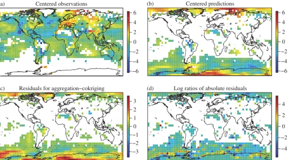
Fig. 5. Centred observed (a) and predicted (b) monthly average temperatures for September 1957 using

AGG( , ω) -cokriging. (c) Prediction errors. The marks indicate the locations for which the

aggregation-cokriging residuals are larger in absolute value compared with the simple kriging ones. (d) Log ratios of the absolute errors ofAGG( , ω) -cokriging and of bikriging with the third variable. The marks indicate the locations for which the aggregation-cokriging residuals are larger in absolute value compared with the bikriging ones.

Figures5(a) and5(b) show the centred observed and predicted monthly average temperatures for September 1957 usingAGG( ,ˆ ω)-cokriging. Figuresˆ 5(c) and5(d) show the prediction errors,

i.e., the difference between the predicted monthly average temperatures for September 1957 using

AGG( ,ˆ ω)-cokriging and the actually observed temperatures. Aggregation-cokriging has a rel-ˆ

ative root average squared prediction error of 0·48. For a simple kriging approach, prediction in high and low latitudes relies only on observations that are far away. With the aggregation-cokriging approach, observations from the secondary variables are available and improve the prediction. The relative root average squared prediction error of the bikriging approaches range from 1·04 to 0·97; see also Table3. There is no structure in the locations where bikriging with the first variable performs better than cokriging. For this application, the aggregation-cokriging performs well because the weighted average smooths the secondary variables close to the poles, which can be interpreted as a regression towards the mean effect.

5. EXTENSIONS

The methodology was applied to gridded temperature anomaly fields from general circu-lation models to construct a best guess reanalysis temperature field. The approach can be applied to other multivariate settings, where we measure different variables on common loca-tions to predict a primary variable. Examples include air pollution data like carbon monox-ide and nitrogen oxmonox-ides to predict tropospheric ozone production (Schmidt & Gelfand, 2003; Majumdar & Gelfand,2007;Apanasovich & Genton,2010) and gridded wind speed and wind direction model data to predict sea surface temperature (Berliner et al., 2000). Ifn+m is too large to solve the associated linear system, it is possible to first apply aggregation-cokriging to

(15)

address the largeℓproblem, and then, for example, employ reduced rank representations of the spatial process (e.g.Banerjee et al.,2008;Cressie & Johannesson,2008) for the bikriging step.

We have assumed that the secondary variables are observed at all the distinctmlocations. If this is not the case, we cannot derive the aggregation matrixAas discussed in§2and it is not possible to derive optimality results. If there are only a few missing values, or the sets of locations are at least similar, we propose to proceed by first kriging the secondary variables to a common set of locations and then apply the aggregation-cokriging procedure.

When the weights do not depend onsp, predicting at more than one location is straightforward

by changing the covariance matrices in (7)–(9) accordingly.

If the primary and the secondary variables have a polynomial or regression type mean, it is possible to formulate the aggregation-cokriging solution as a minimization problem. However, except for very simple or pathological examples, we are not able to formulate closed form expres-sions for the optimal solutions. Nevertheless, the canonical correlation based derivation of the aggregation-cokriging weights can still be made because canonical correlation analysis is mean invariant (Mardia et al.,1979, Theorem 10.2.4).

ACKNOWLEDGEMENT

This research was sponsored by the National Science Foundation, U.S.A., and by an award made by the King Abdullah University of Science and Technology. We acknowledge the inter-national modelling groups for providing their data for analysis. We also thank the editor, the associate editor and two referees for comments that led to a substantial improvement of the paper.

APPENDIX

Throughout the paper and the subsequent proofs, we must evaluate quantities of the form xT C−1w, where the vectors and matrices involved are often partitioned. We first evaluate and simplify such quan-tities. In the following, assume all matrices and vectors have the required dimensions, and are positive definite where required. Then:

xT yT C B BT A −1 x y =x T C−1x+ y−BT C−1x2 E withE=(A−BT_C−1_B₎−1_and_z2

E=zTE z. If Dis a nonsingular matrix, then xT yT DT C B DT D BT _{D A D}T −1 w Dz (A1) =xT C−1w+xT C−1B E BT C−1w−xT C−1B E z−yT ET BC−1w+yT E z. (A2)

Proof of Lemma1. Define the diagonal matrix containing the nonzero scalingsG=diag(γ1, . . . , γm).

Using scalings results in usingGAinstead ofAand we have to prove that (2) and (3) are invariant underG. Both the predictor and the mean squared prediction error are of the form (A1), withDtaking the role ofG. Because (A2) is independent ofD, the prediction and the mean squared prediction error are independent

of the scalingsγ1, . . . , γm.

Proof of Proposition2. With (11), we have ck=ωk(cp−c0−0010p) and Sr s= r scc− ωrωsc0−0010cand (10) may be written as

_ℓ k=1 akωkc˜ T _ℓ r,s=1 aras r scc−arasωrωsS˜ −1 _ℓ l=1 alωkc˜ , at Zentralbibliothek on February 6, 2012 http://biomet.oxfordjournals.org/ Downloaded from

(16)

wherec˜=ck/ωkandS˜=c0−0010c. Similar to Lemma1, we scaleasuch thataTω=1. Hence,

˜ cT₍

aT

acc− ˜S)−1c˜= ˜cTU(λ)−1c˜,

with λ=aT _a _and _U_(λ)₌_λ

cc− ˜S. Note that λ >0 because a=| 0 and U(λ) is positive definite

because (11) is so. For any c˜, maximizing maxλc˜TU(λ)−1c˜ is equivalent to minλc˜TU(λ)c˜ and to

minλλc˜Tccc˜, and to minaλ=minaaT a, yielding the desired result. Proof of Lemma2. Because a(si)T1=| 0, we scale the weight vectors and usea˜i=a(si){a(si)T1}−1.

Then withAbased ona˜iwe have

A(Y0−0010p−Yp)=

ℓ

r=1

diag(Lr)cr=c1,

whereck=k000−10p−kp. LetEA= {A(YY−Y0−0010Y)AT}−1. Equivalent expressions hold

for the second aggregation matrix. We need to show that cT

1EBc1<cT1EAc1 if and only if 0<c1T(EA− EB)c1. Now,EA−EBis positive definite if and only if E−B1−E

−1

A is positive definite (Harville,1997,

Theorem 18.2.4), if and only if

B(YY−Y000−10Y)BT−A(YY−Y000−10Y)AT (A3)

is positive definite. The matrixYY−Y0−0010Yis defined by itsℓ2blocks,r s−r0−0010s, each

being a positive definitem×mmatrix. The second term of the blocks does not depend onsorr. Thus,

A(YY−Y000−10Y)AT= ℓ r=1 ℓ s=1 diag(Lr)(r s−r000−10s)diag(Ls) = ℓ r=1 ℓ s=1 r s◦LrLTs− ℓ r=1 diag(Lr)10−00101 ℓ s=1 diag(Ls) = ℓ r=1 ℓ s=1 r s◦LrLTs.

Therefore, (A3) is positive definite if and only if (12) is positive definite.

Proof of Lemma3. In the case of constant weights given by a(aT

1)−1 and b(bT

1)−1, Gr s= aras(aT1)−211T and accordingly Hr s=brbs(bT1)−211T. Therefore, (12) reduces to ℓr=1

ℓ

s=1r s◦

11T_{

brbs(bT1)−2−aras(aT1)−2}, proving the first statement. A sum of positive definite matrices is

positive definite and the Schur product of a positive definite matrix with a nonnegative definite matrix is positive definite (Horn & Johnson,1994, Theorem 5.2.1), proving the second statement. For the third statement, we write rr=Kr +12, implying

ℓ r=1 ℓ s=1r s=ℓ212+ ℓ r=1Kr. Hence, ℓ r=1 ℓ s=1diag(Lr)r sdiag(Lr)=ℓ212+ℓr=1Kr ◦11Tar2(a T₁₎−2_{, because}ℓ r=1Lr=1. Finally, if rr=11, the problem reduces toℓr=1b2r(b

T₁₎−2₋_a2 r(a

T₁₎−2_{being positive.} Proof of Corollary1. The first item is trivial. In the case of bikriging, b=e1 and the second item

follows immediately from the last statement of Lemma3.

Proof of Proposition3. The matricesCii andCi p defined by (7) and (8) are of the formb1I+b211T andb31. Thus, the vectora=1 is an eigenvector ofCii−1Ci pCpi and because of the symmetry ofCiialso

of C_ii−1/2Ci pCpiCii−1/2 . The covariance structure with (11) implies thatωis proportional to 1 and = αI+β11T_{, for some constants}_α_and_β_{. Recall that the largest eigenvalue of} _is_α₊_ℓβ_{with associated} eigenvector 1. Further,AGG( , ω)-cokriging uses an aggregation vectora= −11(1T −11)−1and with

−1₌_α−1_I₋_β(α2₊_ℓαβ)−1₁₁T_{we can conclude that}_a_{is proportional to 1.}

(17)

We write the covariance between different secondary variables as12and the within covariance of the secondary variables as12+R. For aggregation-cokriging, we useA=1T⊗I to show that

g(1)=m(1p−1000−10p)T(R+m12−10−00101)−1(1p−10−0010p).

For cokriging, we write the matrices with Kronecker products, namely

(Yp−Y0−0010p)T(YY−Y0−0010Y)−1(Yp−Y0−0010p)= {1T⊗(1p−10−0010p)}T ×(I ⊗R+11T⊗12−11T⊗10−00101 −1 {1T_⊗₍ 1p−10−0010p)}T=g(1). REFERENCES

ABOURFIRASSI, M. & MARINO, M. A.(1984). Cokriging of aquifer transmissivities from field measurements of trans-missivity and specific capacity.J. Int. Assoc. Math. Geol.16, 19–35.

APANASOVICH, T. V. & GENTON, M. G.(2010). Cross-covariance functions for multivariate random fields based on latent dimensions.Biometrika97, 15–30.

BANERJEE, S., GELFAND, A. E., FINLEY, A. O. & SANG, H.(2008). Gaussian predictive process models for large spatial

data sets.J. R. Statist. Soc.B70, 825–48.

BERLINER, L. M., WIKLE, C. K. & CRESSIE, N.(2000). Long-lead prediction of Pacific SSTs via Bayesian dynamic

modeling.J. Climate.13, 3953–68.

BILLINGS, S. D., BEATSON, R. K. & NEWSAM, G. N.(2002). Interpolation of geophysical data using continuous global

surfaces.Geophysics67, 1810–22.

BOURGAULT, G. & MARCOTTE, D.(1991). Multivariable variogram and its application to the linear model of

coregion-alization.Math. Geol.23, 899–928.

BROHAN, P., KENNEDYJ. J., HARIS, I., TETT, S. F. B. & JONES, P. D.(2006). Uncertainty estimates in regional and

global observed temperature changes: a new dataset from 1850.J. Geophys. Res.111, D12106.

CARR, J. R. & MCCALLISTER, P. G.(1985). An application of cokriging for estimation of tripartite earthquake response spectra.J. Int. Assoc. Math. Geol.17, 527–45.

CRESSIE, N. A. C.(1993).Statistics for Spatial Data. New York: John Wiley & Sons Inc., revised reprint.

CRESSIE, N. & JOHANNESSON, G.(2008). Fixed rank kriging for very large spatial data sets.J. R. Statist. Soc.B70, 209–26.

DAVIS, B. M. & GREENES, K. A.(1983). Estimation using spatially distributed multivariate data: an example with coal quality.J. Int. Assoc. Math. Geol.15, 291–304.

FURRER, R. & SAIN, S. R.(2010). spam: A sparse matrix R package with emphasis on MCMC methods for Gaussian Markov random fields.J. Statist. Software36, 1–25.

FURRER, R., GENTON, M. G. & NYCHKA, D.(2006). Covariance tapering for interpolation of large spatial datasets. J. Comp. Graph. Statist.15, 502–23.

GELFAND, A., SCHMIDT, A., BANERJEE, S. & SIRMANS, C.(2004). Nonstationary multivariate process modelling

through spatially varying coregionalization (with discussion).Test13, 1–50.

GENTON, M. G.(2007). Separable approximations of space-time covariance matrices.Environmetrics18, 681–95. GNEITING, T.(2002). Compactly supported correlation functions.J. Mult. Anal.83, 493–508.

HAAS, T. C.(1990a). Kriging and automated variogram modeling within a moving window.Atmosph. Envir., Part A

24, 1759–69.

HAAS, T. C.(1990b). Lognormal and moving window methods of estimating acid deposition.J. Am. Statist. Assoc.85,

950–63.

HARVILLE, D. A.(1997).Matrix Algebra From a Statistician’s Perspective. New York: Springer.

HERTZOG, A., BASDEVANT, C. & VIAL, F.(2006). An assessment of ECMWF and NCEP–NCAR reanalyses in the southern hemisphere at the end of the presatellite era: results from the EOLE experiment (1971–72).Mon. Weather Rev.134, 3367–83.

HORN, R. A. & JOHNSON, C. R.(1994).Topics in Matrix Analysis. Cambridge: Cambridge University Press.

JOHNS, C., NYCHKA, D., KITTEL, T. & DALY, C.(2003). Infilling sparse records of spatial fields.J. Am. Statist. Assoc.

98, 796–806.

JOLLIFFE, I. T.(2002).Principal Component Analysis. 2nd ed. New York: Springer.

JONES, P. D., NEW, M., PARKER, D. E., MARTIN, S. & RIGOR, I. G.(1999). Surface air temperature and its variations

over the last 150 years.Rev. Geophys.37, 173–99.

JOURNEL, A. G. & HUIJBREGTS, C. J.(1978).Mining Geostatistics. London: Academic Press.

KALNAY, E., KANAMITSU, M., KISTLER, R., COLLINS, W., DEAVEN, D., GANDIN, L., IREDELL, M., SAHA, S., WHITE, G., WOOLEN, J., ZHU, Y., CHELLIAH, M., EBISUZAKI, W., HIGGINS, W., JANOWIAK, J., MO, K. C., ROPELEWSKI, C.,

(18)

WANG, J., LEETMA, A., REYNOLDS, R., JENNE, R. & JOSEPH, D.(1996). The NCEP/NCAR 40-year reanalysis

project.Bull. Am. Meteor. Soc.77, 437–71.

LONG, A. E. & MYERS, D. E.(1997). A new form of the cokriging equations.Math. Geol.29, 685–703.

MA, L., ZHANG, T., LI, Q., FRAUENFELD, O. W. & QIN, D.(2008). Evaluation of ERA-40, NCEP-1, and NCEP-2

reanalysis air temperatures with ground-based measurements in China.J. Geophys. Res.113, D15115.

MAJUMDAR, A. & GELFAND, A. E.(2007). Multivariate spatial modeling using convolved covariance functions.Math. Geol.39, 225–45.

MARDIA, K. V., KENT, J. T. & BIBBY, J. M.(1979).Multivariate Analysis. London: Academic Press.

MATHERON, G.(1962). Traité de géostatistique appliquée, Tome I.In Mémoires du Bureau de Recherches Géologiques et MinièresNo. 14, Paris: Editions Technip.

MEEHL, G. A., STOCKER, T. F., COLLINS, W. D., FRIEDLINGSTEIN, P., GAYE, A. T., GREGORY, J. M., KITOH, A., KNUTTI, R., MURPHY, J. M., NODA, A., RAPER, S. C. B., WATTERSON, I. G., WEAVER, A. J. & ZHAO, Z.-C.(2007). Global climate projections. InClimate Change 2007: The Physical Science Basis. Contribution of Working Group I to the Fourth Assessment Report of the Intergovernmental Panel on Climate Change, Ed. S. Solomon, D. Qin, M. Manning, Z. Chen, M. Marquis, K. B. Averyt, M. Tignor & H. L. Miller. Cambridge: Cambridge University Press.

MYERS, D. E.(1982). Matrix formulation of co-kriging.J. Int. Assoc. Math. Geol.14, 249–57.

MYERS, D. E.(1983). Estimation of linear combinations and co-kriging.J. Int. Assoc. Math. Geol.15, 633–7. MYERS, D. E.(1992). Kriging, co-kriging, radial basis functions and the role of positive definiteness.Comp. Math.

Appl.24, 139–48.

SCHMIDT, A. & GELFAND, A.(2003). A Bayesian coregionalization approach for multivariate pollutant data.J. Geophy. Res. A108, D24, 8783.

SUN, Y., LI, B. & GENTON, M. G. (2011). Geostatistics for large datasets. InAdvances and Challenges in Space-time Modelling of Natural Events, Ed. J. M. Montero, E. Porcu & M. Schlather. Springer, in press.

http://www.stat.tamu.edu/∼genton/2011.large.book.pdf.

VERHOEF, J. M. & CRESSIE, N.(1993). Multivariable spatial prediction.Math. Geol.25, 219–39. VERHOEF, J. M. & CRESSIE, N.(1994). Errata: multivariable spatial prediction.Math. Geol.26, 273–5.

WACKERNAGEL, H.(2006).Multivariate Geostatistics, 3rd ed. New York: Springer.

[Received September2010. Revised April2011]