Topics in generalized linear mixed models and spatial subgroup analysis

(1)

2018

Topics in generalized linear mixed models and

spatial subgroup analysis

Xin Wang

Iowa State University

Follow this and additional works at:

https://lib.dr.iastate.edu/etd

Part of the

Statistics and Probability Commons

This Dissertation is brought to you for free and open access by the Iowa State University Capstones, Theses and Dissertations at Iowa State University Digital Repository. It has been accepted for inclusion in Graduate Theses and Dissertations by an authorized administrator of Iowa State University Digital Repository. For more information, please [email protected].

Recommended Citation

Wang, Xin, "Topics in generalized linear mixed models and spatial subgroup analysis" (2018).Graduate Theses and Dissertations. 17348.

(2)

by

Xin Wang

A dissertation submitted to the graduate faculty

in partial fulfillment of the requirements for the degree of

DOCTOR OF PHILOSOPHY

Major: Statistics

Program of Study Committee: Zhengyuan Zhu, Co-major Professor Vivekananda Roy, Co-major Professor

Emily Berg Alicia Carriquiry

Huaiqing Wu

The student author, whose presentation of the scholarship herein was approved by the program of study committee, is solely responsible for the content of this

dissertation. The Graduate College will ensure this dissertation is globally accessible and will not permit alterations after a degree is conferred.

Iowa State University

Ames, Iowa

2018

(3)

DEDICATION

(4)

TABLE OF CONTENTS

Page

LIST OF TABLES . . . vi

LIST OF FIGURES . . . viii

ACKNOWLEDGEMENTS . . . x

ABSTRACT . . . xi

CHAPTER 1. OVERVIEW . . . 1

Bibliography . . . 5

CHAPTER 2. A NEW ALGORITHM TO ESTIMATE MONOTONE NONPARAMET-RIC LINK FUNCTIONS AND A COMPARISON WITH PARAMETNONPARAMET-RIC APPROACH 7 2.1 Introduction . . . 8

2.2 Parametric link functions . . . 11

2.2.1 Symmetric link functions . . . 11

2.2.2 Asymmetric link functions . . . 12

2.3 Nonparametric link functions . . . 14

2.4 A new algorithm for estimating monotone link functions . . . 16

2.5 Simulation study . . . 19

2.5.1 Simulation settings . . . 20

2.5.2 Simulation results . . . 23

2.6 Real data analysis . . . 27

2.7 Conclusion and discussion . . . 29

CHAPTER 3. SMALL AREA ESTIMATION OF PROPORTIONS WITH CONSTRAINT FOR NATIONAL RESOURCES INVENTORY SURVEY . . . 33

3.1 Introduction . . . 33

3.2 National Resources Inventory . . . 38

3.3 Spatial Bayesian hierarchical models for proportions . . . 41

3.3.1 Generalized Dirichlet distribution . . . 41

3.3.2 Model specification . . . 42

3.3.3 Bayesian estimation . . . 45

3.4 Design based simulation study . . . 45

3.5 Application to 2012 NRI . . . 49

3.6 Discussion . . . 52

(5)

CHAPTER 4. CONVERGENCE ANALYSIS OF BLOCK GIBBS SAMPLERS FOR

BAYESIAN PROBIT LINEAR MIXED MODELS . . . 57

4.2 Geometric ergodicity of the two-block Gibbs sampler under proper priors . . . 62

4.2.1 A two-block Gibbs sampler . . . 62

4.2.2 Geometric ergodicity of the block Gibbs sampler . . . 64

4.2.3 A Haar PX-DA algorithm . . . 67

4.3 Geometric ergodicity of the two-block Gibbs sampler under improper priors . . . 69

4.3.1 Geometric ergodicity of the block Gibbs sampler . . . 69

4.3.2 A Haar PX-DA algorithm . . . 73

4.4 An example . . . 74

CHAPTER 5. GEOMETRIC ERGODICITY OF P ´OLYA-GAMMA GIBBS SAMPLER FOR BAYESIAN LOGISTIC REGRESSION WITH A FLAT PRIOR . . . 98

5.2 PS&W’s Gibbs sampler . . . 101

5.3 Geometric ergodicity of P´olya-Gamma Gibbs sampler . . . 103

CHAPTER 6. ANALYSIS OF THE P ´OLYA-GAMMA BLOCK GIBBS SAMPLER FOR BAYESIAN LOGISTIC LINEAR MIXED MODELS . . . 116

6.2 Two-block Gibbs sampler . . . 118

6.3 Uniform ergodicity of the two-block Gibbs sampler . . . 120

CHAPTER 7. ESTIMATING SUBGROUPS FOR SPATIAL AREAL DATA WITH RE-PEATED MEASURES . . . 127

7.2 The model and the algorithm . . . 129

7.2.1 The model with repeated measures . . . 129

7.2.2 The algorithm . . . 131 7.3 Theoretical properties . . . 133 7.4 Simulation studies . . . 137 7.4.1 Balanced group . . . 137 7.4.2 Unbalanced group . . . 142 7.4.3 Random group . . . 144

(6)

7.5 Application . . . 145

(7)

LIST OF TABLES

Page

Table 2.1 Considered link functions . . . 23

Table 2.2 Summary of simulation results with sample size 100 . . . 24

Table 2.5 Summary of simulation results with sample size 100 for nonlinear case 2 and case 3 . . . 26

Table 3.1 Model assessmentp-values and DIC values . . . 50

Table 3.2 Estimates of parameters . . . 51

Table 4.1 Results for the block Gibbs sampler and the Haar PX-DA algorithm . . . . 75

Table 4.2 Estimated effective sample sizes per second . . . 77

Table 7.1 Summary of ˆK for the first set of parameters under the 7×7 grid . . . 139

Table 7.2 ARI for the first set of parameters under the 7×7 grid . . . 139

Table 7.3 Summary of ˆK and ARI for the first set of parameters under the 10×10 grid139 Table 7.4 Summary of ˆK for the second set of parameters under the 7×7 grid . . . . 141

Table 7.5 ARI for the second set of parameters under the 7×7 grid . . . 141

Table 7.6 Summary of ˆK and ARI for the second set of parameters under the 10×10 grid . . . 141

(8)

Table 7.7 Summary of ˆK and ARI based on unbalanced setting with ni= 10 . . . 143

Table 7.8 Summary of ˆK and ARI under the 7×7 grid with ni= 10 . . . 144

Table 7.9 Summary of ˆK and ARI under the 7×7 grid with ni= 30 . . . 145

Table 7.10 Estimated coefficients of different groups for equal weight . . . 146

(9)

LIST OF FIGURES

Page

Figure 2.1 Symmetric link functions . . . 12

Figure 2.2 Asymmetric link functions . . . 14

Figure 2.3 Shape of the predictor function in different scenarios . . . 22

Figure 2.4 RMSE of linear case with sample size 500 . . . 25

Figure 2.5 RMSE of nonlinear case 1 with sample size 500 . . . 26

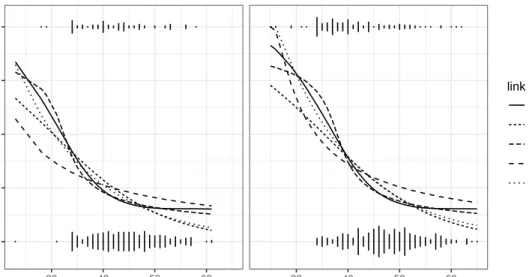
Figure 2.6 The plot of P(yi= 1) under different link functions . . . 28

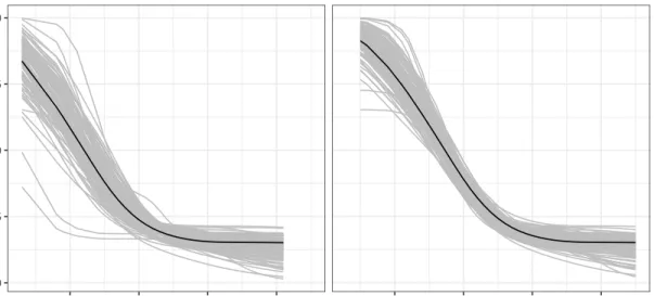
Figure 2.7 Estimated link function from bootstrap samples . . . 29

Figure 3.1 Design RMSE of small area estimators based on different models . . . 47

Figure 3.2 Design relative RMSE of small area estimators based on different models . . 48

Figure 3.3 Estimated maps . . . 51

Figure 3.4 Intervals of cultivated cropland for NRI design based estimates and bench-marked estimates at county level . . . 52

Figure 4.1 Auto-correlation plots of different regression parameters for the three algo-rithms . . . 76

Figure 7.1 Two spatial settings . . . 138

Figure 7.2 RMSE for the first set of parameters under the 7×7 grid . . . 140

Figure 7.3 RMSE for the first set of parameters under the 10×10 grid . . . 140

Figure 7.4 RMSE under the second set of parameters under the 7×7 grid . . . 142

Figure 7.5 RMSE under the second set of parameters under the 10×10 grid . . . 142

Figure 7.6 Unbalanced simulation setting . . . 143

(10)

Figure 7.8 RMSE for random groups under the 7×7 grid . . . 145

Figure 7.10 Estimated groups for both equal weight and spatial weight . . . 147

Figure 7.11 Estimated groups by changing tuning parameter with equal weights . . . 147

(11)

ACKNOWLEDGEMENTS

I would like to take opportunity to thank my advisors Dr. Zhengyuan Zhu and Dr. Vivekananda

Roy for their guidance, patience, encouragement and support during my five years study and

research. Without their help, I cannot complete this work and pursue my career. From them, I

have learned the way and the attitude of doing research.

I would also like to thank my committee members for their efforts and contributions to this

work: Dr. Emily Berg, Dr. Alicia Carriquiry and Dr. Huaiqing Wu. Thank Dr. Emily Berg for

all her kind and great help in my research assistant work. I would also like to thank Dr. Kenneth

Koehler for his guidance of teaching. Additionally, I would like to thank Dr. Dongchu Sun and Dr.

Helen Hao Zhang for their suggestions of my research work.

I would like to thank my parents for their endless love and support. Especially my mother, she

tries to understand my life that is far away from her. I would also like to thank my friends both in

(12)

ABSTRACT

In this thesis, two topics are studied, generalized linear mixed models and spatial subgroup

analysis.

Within the topic of generalized linear mixed models, this thesis focuses on three aspects. First,

estimation of link function in generalized linear models is studied. We propose a new algorithm that

uses P-spline for nonparametrically estimating the link function which is guaranteed to be

mono-tone. We also conduct extensive simulation studies to compare our nonparametric approach with

various parametric approaches. Second, a spatial hierarchical model based on generalized Dirichlet

distribution is developed to construct small area estimators of compositional proportions in the

National Resources Inventory survey. At the observation level, the standard design based

estima-tors of the proportions are assumed to follow the generalized Dirichlet distribution. After proper

transformation of the design based estimators, beta regression is applicable. We consider a logit

mixed model for the expectation of the beta distribution, which incorporates covariates through

fixed effects and spatial effect through a conditionally autoregressive process. Finally, convergence

rates of Markov chain Monte Carlo algorithms for Bayesian generalized linear mixed models are

studied. For Bayesian probit linear mixed models, we construct two-block Gibbs samplers using

the data augmentation (DA) techniques and prove the geometric ergodicity of the Gibbs samplers

under both proper priors and improper priors. We also provide conditions for posterior propriety

when the design matrices take commonly observed forms. For Bayesian logistic regression models,

we establish that the Markov chain underlying Polson et al.’s (2013) DA algorithm is

geometri-cally ergodic under a flat prior. For Bayesian logistic linear mixed models, we construct a two-block

Gibbs sampler using Polson et al.’s (2013) DA technique under proper priors and prove the uniform

(13)

The other topic is spatial subgroup analysis with repeated measures. We use pairwise concave

penalties for the differences among group regression coefficients based on smoothly clipped absolute

deviation penalty. We also consider pairwise weights associated with each paired penalty based on

spatial information. We show that the oracle estimator based on weighted least square is a local

minimizer of the objective function with probability approaching 1 under some conditions. In the

simulation study, we compare the performances of different weights as well as equal weights, which

shows that the spatial information will help when the minimal group difference is small or the

(14)

CHAPTER 1. OVERVIEW

Analyzing non-Gaussian data is an important topic in Statistics. Generalized linear models

(GLMs) and Generalized linear mixed models (GLMMs) are often used. This topic is studied in

both methodological and theoretical aspects. Besides that, spatial subgroup analysis is also studied.

In Chapter 2, we propose a new algorithm to estimate the unknown link function with monotone

constraints in GLMs. In classical GLMs, the link function is assumed to be a known function.

Examples of traditional link functions include logit, probit and the complementary log-log (cloglog)

links. Czado and Santner (1992) showed that misspecification of link function can introduce bias

and increase mean squared error of regression coefficient estimates and the predicted probabilities

for binary data. Flexible families of link functions have been proposed in the literature to address

the misspecification problem. These link functions usually have parameters to control the skewness

of link functions, such as robit link function (Liu, 2004), GEV link function (Wang and Dey,

2010) and symmetric power link family (Jiang et al., 2013). Besides parametric link functions,

Muggeo and Ferrara (2008) proposed a generalized single index model (GSIM), which assumed an

unknown link function with linear predictors. In Muggeo and Ferrara (2008), the link function is

estimated by P-spline (Eilers and Marx, 1996; Eilers et al., 2015) and the monotone assumption

is dealt with by introducing a very large penalty term. The algorithm we propose can be applied

to models with more than one covariate and can estimate the link function and the regression

coefficients simultaneously. The algorithm is an iterative procedure with two steps. The first step

is to estimate the unknown link function. The transformation in Wang and Yang (2009) is used

to restrict the domain of the index. The quadratic optimization based method is then applied to

estimate the monotone link function when fixing the estimates of the regression coefficients, which

can guarantee that we have a monotone link function. The second step is to estimate the regression

(15)

probit, robit, GEV, splogit, generalized additive model with our proposed algorithm in binary data.

The simulation study shows that the nonparametric link function model estimated by our proposed

algorithm has the best overall performance, and can approximate different parametric link functions

very well when the data is simulated from these link functions.

In Chapter 3, a spatial hierarchical model is developed to produce county level estimates for the

National Resources Inventory (NRI) survey. The proposed model is based on a generalized

Dirich-let (GD) distribution to construct small area estimators of compositional proportions in several

mutually exclusive and exhaustive land cover categories. Because of small sample sizes, standard

NRI estimators can have relatively large estimated coefficients of variation at the county level.

Additional sources of information, particularly auxiliary variables and explicit model assumptions,

are needed to improve the precision of the county level estimators. The proposed model has several

characteristics. First, estimators based on the model respect the parameter space for the

propor-tions and satisfy a sum-to-one constraint. Second, the model allows incorporation of covariates

and spatial dependence structures to provide more information to improve the estimators.

Addi-tionally, it can incorporate the estimated variance of the original NRI estimators to appropriately

reflect NRI sample design and estimation procedures. To specify a model appropriate for the NRI

application, we begin with an assumption that the observed county level compositional proportions

are realizations from the GD distribution, which is a flexible distribution for vectors of

composi-tional proportions. The GD assumption permits a transformation of the county level proportions

to independent beta random variables with distinct mean and dispersion parameters. The

expec-tation of the beta distribution is modeled as a logit-linear mixed model with covariates describing

large scale structure and spatially correlated random effects for counties. The spatial structure is

specified through a spatial conditionally autoregressive (CAR) model, as in Banerjee et al. (2014).

Our variance model exploits both the chi-square distribution and the lognormal distribution, which

extends that of Maiti et al. (2014) to incorporate covariates. In a design based evaluation study, the

proposed model based estimators are shown to have smaller root mean squared error and relative

(16)

(L´opez-Vizca´ıno et al., 2013). We also apply the proposed models to estimate the proportions of

area in several broaduses for Iowa counties in 2012.

In Chapter 4, we consider Markov chain Monte Carlo (MCMC) algorithms for exploring the

intractable posterior densities associated with Bayesian probit linear mixed models under both

proper and improper priors on the regression coefficients and variance components. In particular,

we construct two-block Gibbs samplers using the data augmentation (DA) techniques. In order to

provide valid standard errors, we need to establish a central limit theorem (CLT) for the time

aver-age estimators. The only standard method of establishing CLT for MCMC estimators, is to prove

that the underlying Markov chain is geometrically ergodic (Jones and Hobert, 2001). Geometric

ergodicity is also needed for consistently estimating the asymptotic variance in the Markov chain

CLT (Flegal and Jones, 2010). Under proper priors, the Gibbs sampler Markov chain is

geomet-rically ergodic under truncated priors on precision parameters. While under improper priors, the

conditions for geometric convergence are similar to those guaranteeing posterior propriety. We also

provide conditions for posterior propriety when the design matrices take commonly observed forms.

DA algorithms are known to suffer from slow convergence (Meng and Van Dyk, 1999; Van Dyk and

Meng, 2001). The Haar parameter expanded data augmentation (PX-DA) algorithm (Liu and Wu,

1999) is an improvement of the DA algorithm and it has been shown that it is theoretically at least

as good as the DA algorithm (Hobert and Marchev, 2008) in both efficiency and operator norm

ordering. We propose corresponding Haar PX-DA algorithms, which have essentially the same

computational cost as the two-block Gibbs samplers. An example is used to show the efficiency

gain of the Haar PX-DA algorithm over the block Gibbs sampler and the full Gibbs sampler.

In Chapter 5, the MCMC algorithm for Bayesian logistic linear model is studied. Logistic

regression model is the most popular model for analyzing binary data, which is due to the fact

that the expectation of observing 1 has a closed form as a function of linear predictors, and it is

also easy to interpret the coefficients in terms of odds ratio. In Bayesian framework, when there is

no prior information available about the parameters, noninformative priors are generally used. A

(17)

flat prior on unknown coefficients. The resulting intractable posterior density can be explored by

running Polson et al.’s (2013) DA algorithm. We establish that the Markov chain underlying Polson

et al.’s (2013) DA algorithm is geometrically ergodic under the necessary and sufficient conditions

for propriety of the posterior density (Chen and Shao, 2001). Proving this theoretical result is

practically important as it ensures the existence of central limit theorems for sample averages under

a finite second moment condition. The CLT in turn allows users of the DA algorithm to calculate

standard errors for posterior estimates. In Chapter 6, we construct a two-block Gibbs sampler using

Polson et al.’s (2013) DA technique for Bayesian logistic linear mixed models with normal priors

on regression parameters and truncated Gamma priors on precision parameters. Furthermore, we

prove the uniform ergodicity of this Gibbs sampler.

In Chapter 7, spatial subgroup analysis with repeated measures is studied. Spatial clustering

or spatial boundaries detection is an important problem in disease mapping, spatial epidemiology

and population genetics (Hegarty and Barry, 2008; Reich and Bondell, 2011; Lawson, 2013; Li

et al., 2015). Ma and Huang (2016) and Ma and Huang (2017) considered the problem in linear

regression settings and used the smoothly clipped absolute deviation penalty (Fan and Li, 2001) and

the minimax concave penalty (Zhang, 2010). In spatial data analysis, observations near each other

could share similar patterns. So spatial dependence information should be considered in models to

find homogeneous groups. We consider a spatial clustering or spatial subgroup analysis problem

based on regression coefficients for spatial areal data with repeated measures. We use pairwise

concave penalties for the differences among group (cluster) regression coefficients. We also consider

pairwise weights associated with each paired penalty based on spatial information. Theoretical

properties of the proposed estimators are proved. Besides that, several different pairwise weights

are studied in the simulation study according to the estimated number of groups, root mean square

error and adjusted Rand index. The results show that the spatial information will help when the

minimal group difference is small, or the number of repeated measures is small. An example is also

(18)

Bibliography

Banerjee, S., Carlin, B. P., and Gelfand, A. E. (2014).Hierarchical modeling and analysis for spatial data. Crc Press.

Chen, M.-H. and Shao, Q.-M. (2001). Propriety of posterior distribution for dichotomous quantal response models. Proceedings of the American Mathematical Society, 129(1):293–302.

Czado, C. and Santner, T. J. (1992). The effect of link misspecification on binary regression inference. Journal of statistical planning and inference, 33(2):213–231.

Eilers, P. H. and Marx, B. D. (1996). Flexible smoothing with B-splines and penalties. Statistical science, 11(2):89–121.

Eilers, P. H., Marx, B. D., and Durb´an, M. (2015). Twenty years of P-splines. SORT-Statistics and Operations Research Transactions, 39(2):149–186.

Fan, J. and Li, R. (2001). Variable selection via nonconcave penalized likelihood and its oracle properties. Journal of the American statistical Association, 96(456):1348–1360.

Flegal, J. M. and Jones, G. L. (2010). Batch means and spectral variance estimators in Markov chain Monte Carlo. The Annals of Statistics, 38(2):1034–1070.

Hegarty, A. and Barry, D. (2008). Bayesian disease mapping using product partition models. Statistics in medicine, 27(19):3868–3893.

Hobert, J. P. and Marchev, D. (2008). A theoretical comparison of the data augmentation, marginal augmentation and PX-DA algorithms. The Annals of Statistics, 36(2):532–554.

Jiang, X., Dey, D. K., Prunier, R., Wilson, A. M., and Holsinger, K. E. (2013). A new class of flexible link functions with application to species co-occurrence in cape floristic region. The Annals of Applied Statistics, 7(4):2180–2204.

Jones, G. L. and Hobert, J. P. (2001). Honest exploration of intractable probability distributions via Markov chain Monte Carlo. Statistical Science, 16(4):312–334.

Lawson, A. B. (2013). Bayesian disease mapping: hierarchical modeling in spatial epidemiology. CRC press.

Liu, C. (2004). Robit regression: a simple robust alternative to logistic and probit regression. In Applied Bayesian modeling and causal inference from incomplete-data perspectives, pages 227– 238. Wiley: London.

Liu, J. S. and Wu, Y. N. (1999). Parameter expansion for data augmentation. Journal of the American Statistical Association, 94(448):1264–1274.

L´opez-Vizca´ıno, E., Lombard´ıa, M. J., and Morales, D. (2013). Multinomial-based small area estimation of labour force indicators. Statistical modelling, 13(2):153–178.

(19)

Ma, S. and Huang, J. (2016). Estimating subgroup-specific treatment effects via concave fusion. arXiv preprint arXiv:1607.03717.

Ma, S. and Huang, J. (2017). A concave pairwise fusion approach to subgroup analysis. Journal of the American Statistical Association, 112(517):410–423.

Maiti, T., Ren, H., and Sinha, S. (2014). Prediction error of small area predictors shrinking both means and variances. Scandinavian Journal of Statistics, 41(3):775–790.

Meng, X.-L. and Van Dyk, D. A. (1999). Seeking efficient data augmentation schemes via condi-tional and marginal augmentation. Biometrika, 86:301–320.

Muggeo, V. M. and Ferrara, G. (2008). Fitting generalized linear models with unspecified link function: A P-spline approach. Computational Statistics & Data Analysis, 52(5):2529–2537.

Polson, N. G., Scott, J. G., and Windle, J. (2013). Bayesian inference for logistic models using P´olya-Gamma latent variables. Journal of the American statistical Association, 108(504):1339– 1349.

Reich, B. J. and Bondell, H. D. (2011). A spatial Dirichlet process mixture model for clustering population genetics data. Biometrics, 67(2):381–390.

Van Dyk, D. A. and Meng, X.-L. (2001). The art of data augmentation (with discussion). Journal of Computational and Graphical Statistics, 10:1–50.

Wang, L. and Yang, L. (2009). Spline estimation of single-index models.Statistica Sinica, 19(2):765– 783.

Wang, X. and Dey, D. K. (2010). Generalized extreme value regression for binary response data: an application to B2B electronic payments system adoption. The Annals of Applied Statistics, 4(4):2000–2023.

Zhang, C.-H. (2010). Nearly unbiased variable selection under minimax concave penalty. The Annals of statistics, 38(2):894–942.

(20)

CHAPTER 2. A NEW ALGORITHM TO ESTIMATE MONOTONE NONPARAMETRIC LINK FUNCTIONS AND A COMPARISON WITH

PARAMETRIC APPROACH

Modified from a paper accepted byStatistics and Computing

Xin Wang1, Vivekananda Roy and Zhengyuan Zhu Department of Statistics, Iowa State University

Abstract

The generalized linear model (GLM) is a class of regression models where the means of the

response variables and the linear predictors are joined through a link function. Standard GLM

assumes the link function is fixed, and one can form more flexible GLM by either estimating the

flexible link function from a parametric family of link functions or estimating it nonparametically.

In this paper, we propose a new algorithm that uses P-spline for nonparametrically estimating the

link function which is guaranteed to be monotone. It is equivalent to fit the generalized single index

model with monotonicity constraint. We also conduct extensive simulation studies to compare our

nonparametric approach for estimating link function with various parametric approaches, including

traditional logit, probit and robit link functions, and two recently developed link functions, the

generalized extreme value link and the symmetric power logit link. The simulation study shows

that the link function estimated nonparametrically by our proposed algorithm performs well under

a wide range of different true link functions and outperforms parametric approaches when they are

misspecified. A real data example is used to illustrate the results.

key words: Generalized linear model; Monotone link functions; P-spline; Single index model;

Skewed link functions

1

(21)

2.1 Introduction

In the generalized linear model (GLM) setup, a link function is used to link the predictors and

the expectation of the response variable (McCullagh and Nelder, 1989). In classical GLMs, the

link function is assumed to be a known function. Examples of traditional link functions include

logit, probit and the complementary log-log (cloglog) links. Czado and Santner (1992) showed that

misspecification of link function can introduce bias and increase mean squared error of regression

coefficient estimates and the predicted probabilities for binary data. Flexible families of link

func-tions have been proposed in the literature to address the misspecification problem. Pregibon (1980)

considered tests and estimation of link function through model linearization. Aranda-Ordaz (1981)

considered two families of link functions for both symmetric and asymmetric cases. Mallick and

Gelfand (1994) used a mixture beta cumulative distribution with fixed number of components as

a link function. Liu (2004) proposed the robit link function which assumes the link function to be

the inverse cumulative distribution function (CDF) of a tdistribution with the degrees of freedom

as a parameter. Several algorithms are proposed in the literature to estimate the parameters of the

robit model, see, e.g., Liu (2004) and Roy (2014). The robit link function can approximate both

the logit link and the probit link with different values of degrees of freedom. One limitation of the

robit link function is that it is symmetric in the sense that the probabilities going to 0 and 1 have

the same rates (Jiang et al., 2013). Kim et al. (2008) proposed a flexible class of link functions

based on a generalized skewed t distribution. Another skewed link function based on the

general-ized extreme value distribution (GEV) was introduced by Wang and Dey (2010), in which a shape

parameter is used to control the skewness of the link function. They used simulation study to show

that GEV link is a more flexible link function by comparing it with logit, probit and cloglog links

in a Bayesian framework. An undesirable property of the GEV link is that the support of GEV

distribution is not the whole real line. Jiang et al. (2013) proposed a symmetric power link family,

which has a parameter to control the skewness, to analyze a species co-occurrence data set. One of

(22)

function. Both t distribution and exponential distribution can also be used as base functions in

Jiang et al. (2013)’s symmetric power links.

Instead of using flexible link functions, alternately, one can use a simple link function and fit

a more flexible regression model. Hastie and Tibshirani (1990) and Wood (2006) developed the

generalized additive model (GAM), in which they used a traditional fixed link function and fitted

an additive model for the covariates. Some extensions are reviewed in H¨ardle et al. (2012). When

there is one covariate, GAM can be viewed as a GLM with nonparametric link function. When

having more than one covariate, single index model (SIM) can be built. In SIM, the expectation

of the response is modeled ash(Xβ), where h is an unknown function and Xβ is the index. The

inverse of h is equivalent to the link function in GLMs when h is monotone. Ichimura (1993)

and Klein and Spady (1993) discussed SIM estimators for binary data. However, these approaches

cannot guarantee the monotonicity of h. Weisberg and Welsh (1994) proposed a way to estimate

unknown link function in GLM using kernel functions, which does not have monotone constraints

for link function. Muggeo and Ferrara (2008) proposed a generalized single index model (GSIM),

which assumed an unknown link function with linear predictor. In Muggeo and Ferrara (2008), the

link function is estimated by P-spline (Eilers and Marx, 1996; Eilers et al., 2015) and the monotone

assumption is dealt with by introducing a very large penalty term.

The problem of estimating monotone functions have been studied in the literature for a long

time. Ramsay (1988) proposed to estimate nondecreasing functions by using linear combination of

integrated splines with nonnegative coefficients. Ramsay (1998) estimated the monotone function

based on differential equations by using spline base functions in estimation. Wang (2000) extended

Ramsay (1998)’s method to estimate monotone link function in GLMs. B-spline (De Boor, 2001)

is also a tool to estimate monotone functions (He and Shi, 1998; Leitenstorfer and Tutz, 2007). A

new algorithm to estimate monotone link function in GLMs via P-spline, which is based on Taylor

expansion and quadratic optimization, was introduced in Wang and Small (2015). However, these

results are all limited to univariate predictor only. Bollaerts et al. (2006) introduced the monotone

(23)

in Muggeo and Ferrara (2008). This idea is also applied in Eilers et al. (2009) and Marx et al.

(2011).

In this paper, we propose a new algorithm to estimate the unknown link function with monotone

constraints in GLMs. This algorithm can be applied to models with more than one covariate and

can estimate the link function and the regression coefficients simultaneously. The algorithm is an

iterative procedure with two steps. The first step is to estimate the unknown link function. The

transformation in Wang and Yang (2009) is used to restrict the domain of the index. Quadratic

optimization based method is then applied to estimate the monotone link function when fixing the

estimates of the regression coefficients, which can guarantee that we have a monotone link function.

The second step is to estimate the regression coefficients when fixing the link function.

As mentioned above, a lot of parametric link functions have been proposed in the literature.

Unfortunately, there does not seem to be any comprehensive studies comparing these parametric

link functions and our nonparametric link functions when fitting GLMs. One of the goals of the

current paper is to undertake an extensive simulation study to compare the performance of

tradi-tional link functions, the recently proposed flexible parametric link functions and nonparametric

link function in terms of prediction accuracy. We use simulation study to compare logit, probit,

robit, GEV, splogit, GAM with our proposed algorithm in binary data. The simulation study

shows that the nonparametric link function model estimated by our proposed algorithm has the

best overall performance, and can approximate different parametric link functions very well when

the data are simulated from these link functions.

The rest of the paper is organized as follows. In Section 2.2, different parametric link functions

are reviewed. In Section 2.3, we review existing nonparametric methods for estimating link

func-tions. In Section2.4, we describe the new algorithm to estimate monotone unknown link functions

in GLMs. Simulation study results are presented in Section2.5, where the performances of a variety

of link functions are compared under different true links. The results from a real data analysis are

(24)

2.2 Parametric link functions

Let Yi be the response variable for theith observation,xi be the vector of covariates, βbe the

regression coefficients and ηi = x0_iβ for i= 1, . . . , n. We assume that Yi’s are independent with

density,

f(yi|θi, ψi) =d(yi, ψi) exp[(θiyi−b(θi))/a(ψi)],

whereθi andψi are unknown parameters, andψi could be constant in one parameter distributions,

such as the Bernoulli distribution and the binomial distribution (McCullagh and Nelder, 1989).

The functionsa(·) andb(·) are known functions and,

µi ≡ E(Yi) =b0(θi), var(Yi) = b00(θi) a(ψi) = V(µi) a(ψi) .

A link functiong(·) links the expectation µi and the covariates xi through,

g(µi) =ηi≡x0iβ. (2.1)

When g(·) =b0−1(·), thenθi =x0iβand in this case g(·) is called the canonical link for the model.

2.2.1 Symmetric link functions

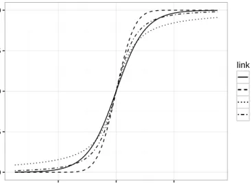
Jiang et al. (2013) provided an interpretation of symmetric and asymmetric link functions. For

symmetric link functions, the probabilities of going to 0 and 1 have the same rates for binary or

binomial variables. Logit, probit and robit link functions are all symmetric link function. Figure

2.1 shows the CDFs corresponding to logit, probit and robit with degrees of freedom 1 and 2. All

of them go through the point (0,0.5). And they are symmetric with respect to (0,0.5).

For logit link function, we have g(µi) = log(µi/(1−µi)), which is a closed form and is easy

to deal with. If g(µi) = Φ−1(µi), then we have the probit regression model, where Φ(·) is the

CDF of the standard normal distribution. Both logit and probit link functions are completely

known; there is no parameter to estimate in these link functions. On the other hand, the robit link

(25)

0.00 0.25 0.50 0.75 1.00 −4 0 4 x P(Y=1) link logit probit ν=1 ν=2

Figure 2.1: Symmetric link functions

parameter ν. EM-type algorithms can be used to estimate both the value of degrees of freedom

parameter and the regression coefficients (Liu, 2004).

2.2.2 Asymmetric link functions

An example of traditional asymmetric link function is cloglog link, g(µi) = −log(−log(µi)),

which does not have any parameters to control the skewness of the link function. By introducing

parameters in the link function, we can have flexible asymmetric link functions, such as the

gener-alized skewed t link in Kim et al. (2008), the GEV link in Wang and Dey (2010) and the splogit

link in Jiang et al. (2013).

Wang and Dey (2010)’s GEV link is given by,

g−1(ηi) = 1−Gξ(−ηi), (2.2)

whereGξ(·) is the cumulative distribution function of the GEV distribution with center parameter

0, scale parameter 1 and shape parameter ξ, i.e., Gξ(x) = exp[−{1 +ξx}

−1/ξ

+ ], where {z}+ =

max{z,0}. In Wang and Dey (2010), the parameters of the model are estimated under Bayesian

(26)

instead of using a Bayesian method. Since the support of GEV is{x: 1+ξx≥0}, we use R package

nloptr (Ypma, 2014) to solve the optimization problem with constraints{β: 1−ξx0_iβ≥0}. Wang

and Dey (2010) used the definition of skewness of a random variable as γM = 1−2F(Mx), where

F is the CDF of the random variable and Mx is the mode. The GEV link in (2.2) is negatively

skewed whenξ <log 2−1 and positively skewed when ξ >log 2−1. They used simulation study

and a real data set to show that GEV link function can approximate probit and logit links well.

Besides that, GEV can improve the results of cloglog for imbalanced data.

For the symmetric power link, we have g(µi) =Fr−1(µi) (Jiang et al., 2013) with

Fr(x) = F0r _x r I(0,1](r) + [1−F 1/r 0 (−rx)]I(1,+∞)(r),

where F0(x) is a base function, and r is the parameter which controls the skewness of the link

function. The function F0(x) can be the CDF of the logistic distribution, t distribution or the

exponential distribution. Jiang et al. (2013) considered a Bayesian analysis of binomial data using

the symmetric power links. Here we consider logistic distribution only and the corresponding splogit

links. One problem of this link function is that splogit link is continuous at r = 1, but it is not

differentiable. In this paper, we maximize the profile likelihood of r to do estimation, that is, we

estimate r by, ˆ r = arg max r p(r), where, p(r) = arg max β n X i=1 yilog Fr(x0iβ) 1−Fr(x0iβ) + n X i=1 log(1−Fr(x0iβ)).

Jiang et al. (2013) compared splogit link and GEV link when simulating data from logit, cloglog

and log-log link models. Splogit performs better than GEV when the true link function is logit or

log-log and GEV link performs better when the true link is cloglog.

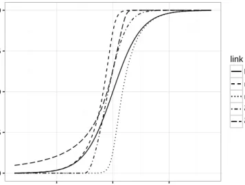
Figure 2.2 shows the CDFs of GEV link function and the splogit link function with different

values of ξ and r. They do not go through the point (0,0.5) and the rate at which they go to 0 is

different from the rate going to 1. For example, the GEV link withξ= 0.5 goes to 1 at faster rate

(27)

0.00 0.25 0.50 0.75 1.00 −4 0 4 x P(Y=1) link logit r = 0.2 r=5 ξ=−0.5 ξ=0.5

Figure 2.2: Asymmetric link functions

2.3 Nonparametric link functions

In section2.2, we discussed several parametric link functions. In many cases, it is not clear which

parametric link function is more suitable, then one can estimate the link function nonparametrically.

Weisberg and Welsh (1994) used kernel method to estimate the unknown link function. They started

from the expectation and variance structure with the following form,

E(Yi) = g∗(xTi β),

Var(Yi) = σ2V(g∗(xTi β)).

The algorithm is a two-step iteration procedure. The first step is to updateβwhen fixingg∗(·).

The second step is to update the g∗(·) when fixing β. In fact, the estimated function is the inverse

of the link function g(·) defined in (2.1). Since the kernel smoothing method is used to do the

estimation, the monotonicity cannot be guaranteed.

We now describe the generalized single index model (GSIM) proposed in Muggeo and Ferrara

(2008) for binary data. They considered,

(28)

where logit(µi) = log(µi/(1−µi)) andφ(·) is an unknown function, which is estimated by P-spline.

The link function for this model is g(µi) = φ−1(logit(µi)). They used a two steps algorithm to

fit the GSIM. When fixingg(·), the estimation problem becomes a common GLM problem, where

iterative weighted least squares (McCullagh and Nelder, 1989) is used to update the estimates of

β. When fixing β, the unknown function g(·) is estimated by P-spline (Eilers and Marx, 1996).

More specially, Muggeo and Ferrara (2008) considered

logit(µi) =φ(x0iβ) =B(x

0

iβ)δ,

whereB(·)_n×(K+1)is the B-spline basis matrix with theith rowB(x0iβ) = (B0,p(x0iβ), . . . , BK,p(x0iβ)),

p is the degree of the basis functions and δ= (δ0, δ1, . . . , δK)0. The number K is the sum of p and

the number of interior knots.

Iterative weighted least squares is used to update the estimation ofδ, which is similar to Eilers

and Marx (1996). Besides the set of constraints for δ in P-spline with second order, they used

another set of constraints for the monotone functions. The monotone constraints are obtained by

assuming nonnegative or nonpositive derivative of a function. Based on the properties of B-spline

(De Boor, 2001), we can write the derivative ofBδ as,

d dx K X k=0 δkBk,p(x) = 1 h K−1 X k=0 Bk,p−1(x)(δk+1−δk),

whereBis based on equally spaced knots withhas the distance between consecutive interior knots.

Since all the values of B-spline basis functions are nonnegative, the nonnegative monotonic

constraints forδ areδk+1−δk≥0, which can be written as,

Aδ=               −1 1 0 · · · 0 0 0 −1 1 · · · 0 0 0 0 −1 · · · 0 0 .. . ... ... ... ... ... 0 0 0 0 −1 1               δ≥0.

Muggeo and Ferrara (2008) dealt with the monotone constraints by including a very large

(29)

δK−1 < 0)) and I(·) is the indicator function. Here κ is a tuning parameter which controls the

cost of violating the monotonicity constraints. But, we found that the monotonicity may not be

satisfied in some cases, which may depend on the tuning parameterλ and the sample sizen. The

new algorithm we propose in the next section does not suffer from such problem.

2.4 A new algorithm for estimating monotone link functions

The new algorithm contains two steps, which is similar to the algorithm in Muggeo and Ferrara

(2008). But there are two main differences. The first one is the constraint for β. Muggeo and

Ferrara (2008) standardized x0β in every iteration. Here we follow the constraints ||β|| = 1 and

the transformation in Wang and Yang (2009) before using the P-spline to estimate φ(·), where

β = (β1, . . . , βd)T. No intercept is included in β. The transformation is defined as U(·), which is

the rescaled centered beta cumulative distribution function with,

U(η) =Fd(η) = Z η a −1 Γ(d+ 1) Γ(d+1₂ )2₂d(1−t 2₎d−₂1_dt,

whereη ∈[−a, a],d is the dimension ofβ. As mentioned in Wang and Yang (2009), the

transfor-mation U has a quasi-uniform [0,1] distribution, which makes it reasonable to use equally spaced

knots. Then, (2.3) becomes,

g0(µi) =φ(U(ηi)) =B(U(ηi))δ.

where ηi =x0iβ,g0 is a known function which can define the range of µi. In particular,g0 can be

the canonical link function. For example, in binary data, we can use logit as g0, which can make

sure that the value of µi is between 0 and 1. B(x)n×(K+1) corresponds to spline functions. The

transformation considered can make the values of U(x0_iβ) not too extreme. In Wang and Yang

(2009), they used 95th percentile of {||xi||}ni=1 as the value of a. Since we use the constraints

||β||= 1, we have||x0_iβ|| ≤ ||xi||. We use the maximum value of||xi||asain simulation study and

(30)

The second difference is that instead of using a large penalty to force the estimated function

to be close to a monotone function, we use Taylor expansion and iterative quadratic optimization

described in Wang and Small (2015) to solve the constrained optimization problem directly.

In the first step, β is fixed, and then, the problem becomes fitting a generalized linear model

g0(µi) =Bδ (2.4)

with constraints and penalties onδ. The monotone constraint for the link function is denoted as

Aδ≥0 in section 2.3. The penalty is P-spline associated withD,

D=               1 −2 1 · · · 0 0 1 −2 · · · 0 .. . ... ... ... ... 0 0 −2 1 0 0 0 1 −2 1               .

In Muggeo and Ferrara (2008), the δ is updated by,

ˆ

δ= (B0W˜ δB+λD0D+κA0V A)−1B0W˜ δy. (2.5)

We update δby solving the iterative quadratic optimization. The problem in (2.4) with monotone

constraints can be solved by,

min δ − h (y−µ˜) ˜d+ ˜WδBδ˜i0Bδ+1 2δ 0 (B0W˜ δB+λD0D)δ, (2.6)

where ˜d,µ˜,W˜ δ _{and ˜}_δ _{are from previous step, (}_y₋_µ_˜_{) ˜}_d _{are coordinate-wise product and ˜}_Wδ ₌

diag(w₁δ, . . . , w_nδ), ˜d= ( ˜d1, . . . ,d˜n)0, where, wδ_i = " dηi dµi 2 V(µi) #−1 µi=˜µi , ˜ di = V(µi) dηi dµi −1 µi=˜µi .

(31)

Note that (2.6) can be solved by quadratic programming. For example, letg0(µi) =ηi and g0(·) =

logit(·), for binary data, we have,

dηi dµi = 1 µi(1−µi) , V(µi) = µi(1−µi).

So in this casew_iδ= ˜µi(1−µ˜i) and ˜di= 1.

In the second step, δ is fixed. Then, the problem becomes fitting a GLM with a fixed link

function

q−1(g0(µi)) =x0iβ,

where q(·) =φ(U(·)). We use the revised Newton method (Boyd and Vandenberghe, 2004)

men-tioned below to updateβ in Algorithm 2.1.

Algorithm 2.1 Revised Newton method for updating β

1: 1: Compute ∆β = (X0W˜ βX)−1X0W˜ βzβ, where ˜Wβ = diag(w1β, . . . , wβn), zβ = (z β

1, . . . , zβn)0, and w_iβ,z_iβ are defined as,

wβ_i = " _dη i dµi 2 V(µi) #−1 (φ0)2(U0)2 µi=˜µi zβ_i = (yi−µ˜i) dηi dµi ·[φ0U0]−1.

2: 2: Let ∇_l = X0W˜ βzβ and choose the step size t by backtracking line search (Boyd and Vandenberghe, 2004).

3: 2.1: Start fromt= 1, lett=γt.

4: 2.2: Setβnew=βold+t∆_β.

5: 2.3: Standardizeβnew to make||βˆnew||= 1.

6: 2.4: Repeat previous steps until l(βnew) < l(β) +αt(∇l)T∆_β, where l is the negative log-likelihood and α∈(0,0.5),γ ∈(0,1).

7: 3: Updateβ.

Remark 2.1. In Algorithm 2.1, when t= 1, β is updated with size 1 in the∆β direction. This is equivalent to the results based on the weighted least square, that is ,

(32)

where z =X0βold₊_zβ_{. But in the simulation study, we find that the moving size 1 could be too}

large to have numeric issues with small λ. So we use a backtracking line search method to find a small size t. The results based on backtracking line search and weighted least square are the same with sameλ if both can be evaluated.

Based on the previous two steps, the proposed algorithm which we call MPS has the following

steps in Algorithm 2.2.

Algorithm 2.2 The MPS algorithm for estimating unknown link function

1: Start with initial values for ˆβ and ˆδ.

2: Given current ˆβ(m) and ˆδ(m), calculatex0_iβˆ(m). Then updateδ by solving (2.6).

3: Given current ˆβ(m) and ˆδ(m+1), updateβ using the revised Newton method.

4: Repeat previous two steps until some convergence criterion is met.

Initial values for β can be chosen by fitting a logistic regression model without intercept and

standardizing it such that ||β|| = 1. The initial values for δ are 0’s. Boyd and Vandenberghe

(2004) suggest to choose α between 0.01 and 0.3, γ between 0.1 and 0.8. In our simulation study

and the real data example, we choose α = 0.25 and γ = 0.5, and the convergence criterion is

||θ(m+1)−θ(m)||< , whereθ = (β0,δ0)0 and is a small value. Here we use = 10−8.

As in Muggeo and Ferrara (2008), the variability of the regression coefficients and the link

func-tion can be obtained from a bootstrap approach. That means the MPS is fitted for each bootstrap

sample b= 1, . . . , B to obtain the bootstrap sample distribution of the regression coefficients and

the link function.

2.5 Simulation study

In this section, we use simulation study to compare different parametric link functions and

nonparametric link function estimated by our proposed algorithm MPS. We simulate binary data

from the Bernoulli distribution under different link functions, including logit, probit, robit, GEV

and splogit with different parameters. Models with parametric link functions (logit, probit, robit,

(33)

2.1, a flexible regression model is also a choice to extend the GLM. So the GAM with logit link

(Wood, 2006) is also considered in the simulation study. We compare the performance of different

link functions based on the prediction performance.

2.5.1 Simulation settings

The sample sizes we consider aren= 100, 200 and 500. Letβ= (0,1,1)0, andηi =β0+x1iβ1+

x2iβ2, where x1 is continuous and simulated from N(−0.5,1) satisfying |x1+ 0.5| ≤ 3, the other

variable x2 is a binary variable drawn from Bernoulli(0.5). We assume that Yi0s are independent

Bernoulli(µi) random variables with g(µi) = ηi, where we vary the true link function g(·). The

simulation procedure is as follows.

For m= 1, . . . , M,

1. Simulate x1i ∼N(−0.5,1)I(|x1i+ 0.5| ≤3) and x2i ∼Bern(0.5) fori= 1, . . . , n.

Let xi = (1, x1i, x2i)0. Obtain the sequence xnew1i from min(x1) to max(x1) with length 200

on a regular grid. Combine xnew₁_i with {0,1} for all combinations. That means, for each

xnew₁_i , we can create two vectors with (1, xnew₁_i ,0)0 and (1, xnew₁_i ,1)0. Denoted these vectors

as xj,new, j = 1, . . . ,400. This data set is used to compare the prediction performances of

different link functions.

2. Calculateµ(_im)=g−1(x_iTβ) fori= 1, . . . , nandµ_j,(m_new) =g−1(xT_j,_newβ) forj= 1, . . . n1, where

n1= 400 andg is the specified link function.

3. Simulate y(_im) ∼Bern(µ_i(m)) under specified link function for i= 1, . . . , n.

4. Estimate parameters under different link functions based on data sets with different sample

sizen.

In P-spline method, 9 equally spaced knots are used. Generalized cross validation(Wood,

2008) is used to select the penalty parameterλ, which is given by

(34)

whereτ = trace(C),C= (B0WδB+λD0D)−1_B0_Wδ_B _and_D_{( ˆ}_δ

λ,βˆλ) is the deviance, which is defined as 2(lmax−l( ˆδλ,βˆλ)), where l is the log-likelihood,lmax is the maximum possible

log-likelihood. In binary setting,lmax= 0.

For the estimation of logit and probit, we use the maximum likelihood. For robit, we use

PX-EM algorithm in Liu (2004). For GEV and splogit, we use the methods mentioned in

section 2.2.

5. Predict ˆµ(_j,m_new) = ˆg−1₍_xT

j,newβˆ) ,j = 1, . . . , n1, based on the estimated parameters.

Based on the previous results, we calculate the following three statistics for M = 100,

RMSE = v u u t 1 M n1 M X m=1 n1 X j=1 (ˆµ(_j,m_new) −µ_j,(m_new) )2_, _(2.7) WRMSE = v u u t 1 M M X m=1 n1 X j=1 wj(ˆµ(j,mnew) −µ (m) j,new)2, (2.8) and T C= 1 M n1 M X m=1 n1 X j=1

|max(0.75,µˆ(_j,m_new) )−max(0.75, µ(_j,m_new) )|. (2.9)

In (2.8),wj ∝fnorm(xnew1j ;−0.5,1), wherefnorm(·) is the pdf of the standard normal distribution

and Pn1

j=1wj = 1. The reason we consider the unequal weights is that normal distribution is

a popular assumption in real data analysis. (2.9) measures the tail behavior of the link function

which borrows the idea from survival data analysis (Yuan, 2008). It is used to see how well different

models predict the extreme probabilities.

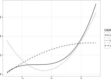
Besides the linear case in η, we also compare the performances of different link functions in

nonlinear case. Here we consider a simple case with one covariate. Three scenarios are considered,

including both monotone and nonmonotonic functions, which we could have in real data examples.

The first one is η = 0.2(x1 + 1)3 −2, the second one is η = x21 +x1 −3, and the third one is

η = −0.2(x1 −3)2 −0.15x21 + 3. The covariate x1 is from the same distribution as in the linear

(35)

monotone. The other two are monotone curves. And the third one is more like a linear line than

the third one. In these three cases, the algorithm is just the first part of the algorithm in section

2.4with updating δ in (2.6), which is just the algorithm in Wang and Small (2015).

For robit link, we consider the degrees of freedom with values 0.6, 1 and 2. When considering

the GEV link function, the shape parameter controls the skewness of the link function. Since the

support of the GEV distribution depends on the unknown location parameter and shape parameter,

different location parameters are taken to avoid the values of η too far away from the support of

the GEV distributions with different shape parameters. In linear case, the location parameters are

-1.5, -1, 0 and 1.2 corresponding to the shape parameters 1, 0.5, -0.5 and -1. For nonlinear cases,

the location parameters are -2, -1, 1 and 1.5 for the same shape parameters. For splogit link, the

consideredr values are 0.2 and 5 in linear case and 0.6 and 1.5 in nonlinear case. For choosing the

penalty parameter λ, we use 100 values between 10−5 _{and 10}12 _{in log}

10 scale.2 −4 0 4 8 −2 0 2 x η case case1 case2 case3

Figure 2.3: Shape of the predictor function in different scenarios

2

In nonlinear case 1, when the true model is probit, the boundary values are 10−5 and 1011, since there are nonpositive definite problem in solve.QR() when theλare too large.

(36)

2.5.2 Simulation results

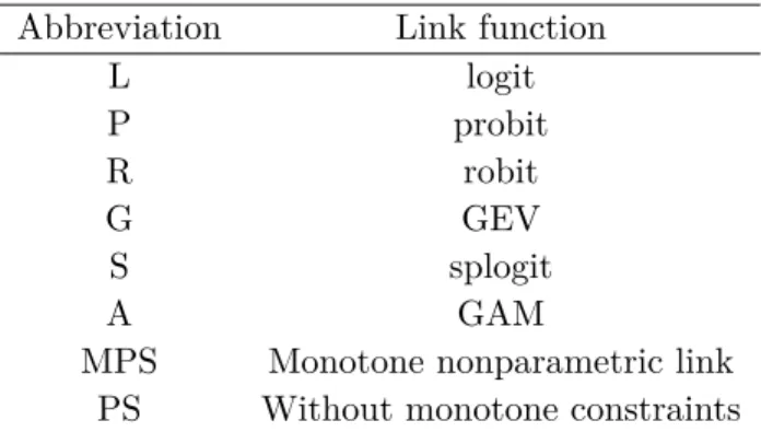
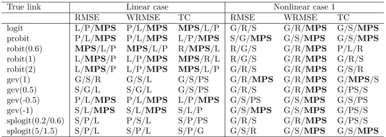
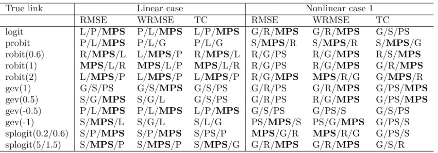
This section shows the results of the simulation study. Table 2.1 gives the abbreviations of

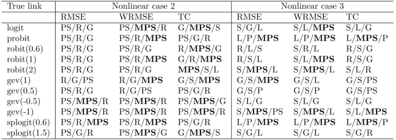
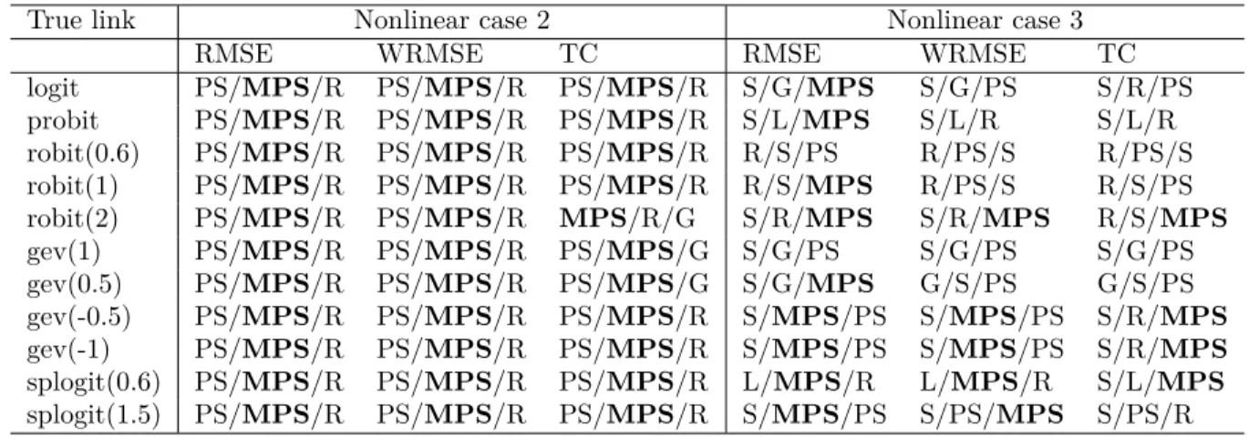
different link functions. Tables 2.2, 2.3 and 2.4 show the simulation results of linear case and

nonlinear case 1. Tables 2.5, 2.6 and 2.7 show the results for nonlinear case 2 and case 3. In

each row, the results are based on different link functions with data simulated from the true

corresponding link function. For example, robit(0.6) row means that the simulated data sets are

simulated under robit link with parameterν = 0.6. Then, we estimate parameters under different

assumptions of link function. If the assumed link function has additional parameter, then the

parameter is estimated as in Section2.2. Figures2.4and2.5show the details of RMSE for selected

true link functions for linear case and nonlinear case 1 with sample size 500.

Table 2.1: Considered link functions

Abbreviation Link function L logit P probit R robit G GEV S splogit A GAM

MPS Monotone nonparametric link PS Without monotone constraints

“PS” can be estimated by the algorithm in (2.5) without the large penalty term and assuming

||β|| = 1 and β1 >0. In each cell, the three link functions are the first three link functions with

smaller value in (2.7), (2.8) and (2.9). For example in the cell with output L/P/MPS, it means

that the model with logit link provides the best result, probit is the second best, and MPS is the

third best.

In most cases of Tables 2.2, 2.3 and 2.4, MPS is in the top three, especially for large sample

sizes. Below we summarize our observations:

1. If the true link function is symmetric, use of asymmetric link function can lead to poor

(37)

2. If the true link function is skewed, then a symmetric link function cannot provide correct

relationship between covariates and the dependent variable.

3. The GEV distribution is approximate symmetric withξ =−0.5. This is why for linear case

and nonlinear case 1, some symmetric link functions can approximate it well when sample

size is 500. For that case, the results of MPS are close to the top three results even though it

is not in the top three (see Supplemental materials). Under both symmetric and asymmetric

true link functions, MPS approach provides reasonable results according to different criteria.

4. For nonlinear case 2, it is quite different from linear function, so the nonparametric method

without constraints performs much better than other parametric link functions.

5. In nonlinear case 3, it is quite similar to linear function,; thus the nonparametric link function

does not have much advantage over the parametric link functions.

Table 2.2: Summary of simulation results with sample size 100

True link Linear case Nonlinear case 1 RMSE WRMSE TC RMSE WRMSE TC

logit L/P/MPS P/L/MPS MPS/L/P G/R/S G/R/MPS G/S/MPS probit P/L/MPS P/L/MPS L/P/MPS S/G/MPS G/S/MPS G/S/MPS robit(0.6) MPS/L/P MPS/L/P R/MPS/L R/G/S G/R/MPS P/L/R robit(1) L/MPS/P L/P/MPS MPS/R/L R/G/S G/R/MPS G/R/S robit(2) L/MPS/P L/P/MPS MPS/L/P G/R/S G/R/MPS G/S/R gev(1) G/S/R G/S/L G/S/PS G/R/MPS G/R/MPS G/MPS/S gev(0.5) S/G/L S/G/L G/S/PS G/R/S G/R/MPS G/PS/S gev(-0.5) P/L/MPS P/L/MPS L/P/MPS G/S/PS G/S/MPS G/S/PS gev(-1) S/L/MPS S/L/MPS S/L/P G/S/MPS G/S/MPS G/PS/S splogit(0.2/0.6) S/P/L P/S/L S/P/PS G/R/S G/R/MPS G/PS/S splogit(5/1.5) S/P/L S/P/L S/P/G G/S/R G/S/MPS G/S/MPS

(38)

True link Linear case Nonlinear case 1 RMSE WRMSE TC RMSE WRMSE TC logit L/P/MPS P/L/MPS L/P/MPS G/R/MPS G/R/MPS G/S/PS probit P/L/MPS P/L/G P/L/G S/MPS/R S/MPS/R S/MPS/G robit(0.6) R/MPS/L L/MPS/P R/MPS/L R/G/PS R/G/MPS R/S/MPS robit(1) MPS/L/R MPS/L/P MPS/L/R R/G/PS R/G/MPS G/R/MPS robit(2) L/MPS/P L/MPS/P L/MPS/P R/G/MPS MPS/R/G G/MPS/R gev(1) G/S/PS G/S/MPS G/S/PS G/R/PS G/R/MPS G/PS/MPS gev(0.5) S/G/MPS S/G/L G/S/PS G/R/PS R/G/MPS G/PS/MPS gev(-0.5) P/L/MPS P/L/MPS L/P/MPS G/S/PS G/PS/S G/S/PS gev(-1) S/MPS/L S/G/L S/L/G PS/MPS/S PS/G/MPS G/PS/S splogit(0.2/0.6) S/P/MPS S/P/MPS S/PS/P MPS/G/R MPS/R/G G/PS/S splogit(5/1.5) S/MPS/P S/MPS/P S/MPS/G G/R/MPS G/R/MPS G/S/R

True link Linear case Nonlinear case 1 RMSE WRMSE TC RMSE WRMSE TC

logit L/MPS/P L/P/MPS L/MPS/P G/MPS/PS MPS/G/R G/MPS/PS probit P/L/R P/L/R P/L/G MPS/PS/S MPS/R/PS MPS/PS/S robit(0.6) R/MPS/L MPS/R/L R/MPS/L R/G/MPS R/MPS/PS MPS/G/PS robit(1) R/MPS/L MPS/L/R R/L/MPS MPS/R/G MPS/R/PS MPS/G/PS robit(2) MPS/L/R L/MPS/R MPS/L/R MPS/R/PS MPS/R/PS MPS/PS/G gev(1) G/S/PS G/S/PS S/G/PS PS/R/MPS R/MPS/PS PS/G/MPS gev(0.5) S/G/MPS S/G/MPS S/G/PS MPS/PS/G MPS/R/PS PS/MPS/G gev(-0.5) S/P/L P/L/S L/R/P MPS/PS/S MPS/PS/G PS/S/MPS gev(-1) S/PS/MPS S/MPS/PS S/L/A PS/MPS/S PS/MPS/G PS/G/MPS splogit(0.2/0.6) S/MPS/PS S/MPS/PS S/PS/MPS MPS/PS/G MPS/PS/R PS/MPS/G splogit(5/1.5) S/MPS/PS S/MPS/PS S/MPS/PS MPS/G/R MPS/R/G G/MPS/S ● ● ● ●●● ● ● ● ● ● ● ● ● ● ● ● ● ● ● ● ● ● ● ● ● ● ● ● ● ● ● ● ● ● ● ● ● ● ● ● ● ● ● ● ● ● ● ● ● ● ● ● ● ● ● ● ● ● ● ● ● ● ● ● ● ● ● ● ● ● ● ●●● ● ● ● ● ●

logit gev(−1) splogit(0.2)

L P R G S PS MPS A L P R G S PS MPS A L P R G S PS MPS A 0.0 0.1 0.2 0.0 0.1 0.2 0.3 0.00 0.05 0.10 0.15 0.20 0.25 assumption RMSE

(39)

Table 2.5: Summary of simulation results with sample size 100 for nonlinear case 2 and case 3

True link Nonlinear case 2 Nonlinear case 3 RMSE WRMSE TC RMSE WRMSE TC logit PS/R/G PS/MPS/R G/MPS/S S/G/L S/L/MPS S/L/G probit PS/R/G PS/R/MPS PS/G/R L/P/MPS L/P/MPS L/MPS/P robit(0.6) PS/R/G PS/R/G R/MPS/G R/L/S S/R/L R/S/G robit(1) PS/R/G PS/R/MPS G/R/MPS R/S/L S/L/MPS R/S/G robit(2) PS/R/G PS/R/G MPS/S/L S/MPS/L S/MPS/L S/L/R gev(1) R/G/PS R/G/MPS G/S/MPS G/S/MPS G/S/L G/S/PS gev(0.5) PS/R/G R/G/PS PS/G/R G/S/P G/S/P G/S/PS gev(-0.5) PS/MPS/R PS/MPS/R PS/MPS/G S/L/G S/L/G S/L/G gev(-1) PS/MPS/R PS/MPS/R PS/MPS/R S/MPS/PS S/MPS/L S/L/MPS splogit(0.6) PS/R/MPS PS/R/MPS PS/G/R L/P/MPS L/P/MPS L/MPS/P splogit(1.5) PS/G/R PS/MPS/G G/MPS/S S/G/L S/G/L S/G/R

True link Nonlinear case 2 Nonlinear case 3 RMSE WRMSE TC RMSE WRMSE TC logit PS/R/MPS PS/MPS/R PS/G/R S/G/L S/G/L S/L/R probit PS/R/MPS PS/MPS/R PS/R/MPS L/MPS/P L/MPS/P L/S/MPS robit(0.6) PS/R/MPS PS/R/MPS R/G/PS R/S/L R/S/PS R/S/G robit(1) PS/R/MPS PS/MPS/R PS/R/G R/S/L R/S/MPS R/S/G robit(2) PS/R/G PS/R/MPS R/S/L S/MPS/R S/MPS/R S/R/L gev(1) PS/R/G PS/R/G PS/G/R G/S/MPS G/S/PS G/S/PS gev(0.5) PS/R/G PS/R/MPS PS/G/R G/S/MPS G/S/P G/S/PS gev(-0.5) PS/MPS/R PS/MPS/R PS/MPS/R S/MPS/L S/MPS/L S/L/R gev(-1) PS/MPS/R PS/MPS/R PS/MPS/R S/MPS/PS S/MPS/PS S/R/MPS splogit(0.6) PS/R/MPS PS/MPS/R PS/MPS/R L/MPS/R L/MPS/R L/S/MPS splogit(1.5) PS/R/MPS PS/MPS/R G/R/PS S/G/MPS S/G/MPS S/R/G ● ● ● ● ● ● ● ● ● ● ● ● ● ● ● ● ● ● ● ● ● ● ● ● ● ● ● ● ● ● ● ● ● ● ● ● ● ● ● ● ● ● ● ● ● ● ● ● ● ● ● ●

logit gev(−1) splogit(0.6)

L P R G S PS MPS L P R G S PS MPS L P R G S PS MPS 0.05 0.10 0.15 0.20 0.025 0.050 0.075 0.100 0.125 0.00 0.05 0.10 0.15 0.20 0.25 assumption RMSE

(40)

True link Nonlinear case 2 Nonlinear case 3 RMSE WRMSE TC RMSE WRMSE TC logit PS/MPS/R PS/MPS/R PS/MPS/R S/G/MPS S/G/PS S/R/PS probit PS/MPS/R PS/MPS/R PS/MPS/R S/L/MPS S/L/R S/L/R robit(0.6) PS/MPS/R PS/MPS/R PS/MPS/R R/S/PS R/PS/S R/PS/S robit(1) PS/MPS/R PS/MPS/R PS/MPS/R R/S/MPS R/PS/S R/S/PS robit(2) PS/MPS/R PS/MPS/R MPS/R/G S/R/MPS S/R/MPS R/S/MPS gev(1) PS/MPS/R PS/MPS/R PS/MPS/G S/G/PS S/G/PS S/G/PS gev(0.5) PS/MPS/R PS/MPS/R PS/MPS/G S/G/MPS G/S/PS G/S/PS gev(-0.5) PS/MPS/R PS/MPS/R PS/MPS/R S/MPS/PS S/MPS/PS S/R/MPS gev(-1) PS/MPS/R PS/MPS/R PS/MPS/R S/MPS/PS S/MPS/PS S/R/MPS splogit(0.6) PS/MPS/R PS/MPS/R PS/MPS/R L/MPS/R L/MPS/R S/L/MPS splogit(1.5) PS/MPS/R PS/MPS/R PS/MPS/R S/MPS/PS S/PS/MPS S/PS/R

2.6 Real data analysis

In this section, we use the data from Muggeo and Ferrara (2008) with sample size n = 683

to compare the models considered in section 2.5.2. The data set is available at http://www.

econ.uiuc.edu/˜roger/courses/471/data/weco.dat, which is used to study the quit behavior

of production workers. The response variable is binary with yi = 1 if the worker quits within six

months of starting a new job, 0 otherwise.

The model we fit in MPS is,

logit(µi) =φ(U(β1x1+β2x2)),

where φ(·) is an unknown function which is estimated by P-spline, U(·) is the rescaled centered

beta cumulative distribution function given in section 2.4, and the constraint for coefficients is

β₁2+β₂2 = 1. The variable x1 denotes sex with 1 for males and 0 for females and the variable x2

denotes the dexterity test score.

A fivefold cross-validation is conducted to compare the performance of different models. The

average misclassification rates for logit, probit, robit, GEV, splogit, the monotone nonparametric

link (MPS) and GAM are 0.253, 0.252, 0.243, 0.253. 0.248, 0.243 and 0.251, respectively. The

additional parameter in link function is estimated together with the regression coefficients according